Study of the finite temperature transition in 3-flavor QCD using the R and RHMC algorithms

Abstract

We study the finite temperature transition in QCD with three flavors of equal masses using the R and RHMC algorithm on lattices with temporal extent $N_{\tau}=4$ and $6$. For the transition temperature in the continuum limit we find $r_{0}T_{c}=0.429(8)$ for the light pseudo-scalar mass corresponding to the end point of the 1st order transition region. When comparing the results obtained with the R and RHMC algorithms for p4fat3 action we see no significant step-size errors down to a lightest pseudo-scalar mass of $m_{ps}r_{0}=0.4$.

I Introduction

Lattice QCD has established the existence of a transition from hadron gas to a new state of strongly interacting matter where quarks and gluons are no longer confined inside hadrons and which is usually called the quark gluon plasma cargese ; reviews . The nature of this transition depends on the quark content and quark masses. For infinite or very large quark masses the transition is a 1st order deconfining transition. In the opposite case of zero quark masses one may have a 2nd order chiral phase transition for 2 flavors or a 1st order chiral phase transition for 3 flavors. For intermediate masses the transition is just a rapid crossover, meaning that thermodynamic quantities change very rapidly in a narrow temperature interval. The boundary of the 1st order transition region of 3 flavor QCD as a function of mass has been studied using improved (p4) karschlat03 and standard staggered actions christian ; norman . There is a significant discrepancy regarding the value of the quark masses, or equivalently the value of the pseudo-scalar meson masses where the transition changes from crossover to 1st order. With an improved action it was found that the 1st order transition ends for a pseudo-scalar meson mass of about $70$ MeV, while with the standard action it ends for pseudo-scalar meson masses of about $190$ MeV christian ; phil2 or larger norman .

It has been observed that the pressure and energy density normalized by its ideal gas value shows almost the same behavior as a function of $T/T_{c}$ for SU(3) pure gauge theory, 2 flavor, 2+1 flavor and 3 flavor QCD cargese . Thus flavor and quark mass dependence of these quantities in the first approximation, is determined by flavor and quark mass dependence of transition temperature $T_{c}$. Therefore it is very instructive to study the flavor dependence of the transition temperature. Such a study has been performed in Ref. karsch01 on lattices with temporal extent $N_{\tau}=4$ using the improved staggered p4 action.

In the past most simulations with 2 and 3 flavors of staggered fermions have been done using the hybrid molecular dynamics R (HMDR) algorithm hybrid , often called simply the R-algorithm. It has finite step-size errors of ${\cal O}(dt^{2})$ where a step-size $dt$ is used in the molecular dynamics evolution. Recently the rational hybrid Monte Carlo (RHMC) algorithm has been invented which allows simulations of theories with fractional powers of the fermion determinant, for example 2 and 3 flavors of staggered fermions, without finite step-size errors rhmc . Therefore the most recent thermodynamics studies use the RHMC algorithm aoki06 ; philipsen06 ; SK06 ; us . It has been observed in Ref. philipsen06 that the use of the exact RHMC algorithm reduces the value of the critical quark mass where the transition turns to 1st order by $25\%$ in the case of the standard staggered action.

The purpose of this paper is twofold. First we would like to study the transition in 3 flavor QCD, extending the previous studies to smaller quark masses and smaller lattice spacings using the improved p4 staggered fermion action. Second we would like to compare the R-algorithm with the new RHMC algorithm. The rest of the paper is organized as follows. In section II we discuss the calculational set-up. In section III we show our results for finite temperature calculations. Section IV discusses the zero temperature simulations needed to set the scale and the transition temperature in physical units. In section V we present a comparison of the R and RHMC algorithms. Finally, section VI contains our conclusions. A technical discussion of different fat link actions is given in Appendix A. In Appendix B we discuss the eigenvalues and eigenvectors of the p4 action in the free field limit.

II Lattice Formulation and setup

Most of the simulations discussed in this paper were done using the p4fat3 action, which is also simply called the p4 action karsch01 . To improve the rotational symmetry, which is violated on the lattice, bent 3-link terms are added to the 1-link term of the standard staggered action Heller . Properly chosen coefficients of the 1-link and the 3-link terms can eliminate, at tree level, the ${\cal O}(a^{2})$ errors in the dispersion relation for staggered fermions Heller . The violation of flavor symmetry which is present in the staggered fermion formulation can be significantly reduced by replacing the normal link in the 1-link term by a fat link which is a sum a of normal link and 3-link staples tb97 . This 3-link fattening is the origin of the name p4fat3. Though this type of fat link action is a big improvement over the standard staggered fermion action, further improvement of the flavor symmetry can be obtained by adding 5- and 7-link staples kostas . In fact one can eliminate the effect of flavor symmetry breaking at order ${\cal O}(g^{2}a^{2})$ using a suitable combination of 3-, 5- and 7- link staples leading to what is called the fat7 action kostas . We have also done calculations with the p4 action with fat7 fat links. Unfortunately it turns out that on the coarse lattices used in our study of 3 flavor QCD thermodynamics this action has some undesirable features. It leads to the occurrence of a bulk transition, which we will discuss in more detail in Appendix A.

To study staggered fermions with less than four flavors, we use the rooting procedure, i.e. each fermion flavor is represented by $({\rm det}\mathcal{M})^{1/4}$, where $\mathcal{M}$ is the staggered fermion Dirac operator. For a recent discussion of this procedure see Ref. sharpe . Most of our simulations have been done using the standard R-algorithm hybrid . As in Ref. karsch01 the step-size of the molecular dynamics evolution was set to $dt=m/2.5$ for the staggered quark mass $m$.

We also performed calculations with the RHMC algorithm. In this algorithm an optimal rational approximation is used to evaluate the fractional power of the determinant rhmc . More precisely one finds the optimal approximation for $(\mathcal{M}^{\dagger}\mathcal{M})^{\nu}$ where $\mathcal{M}=2m+D$ is the usual staggered fermion matrix and for the three flavors $\nu=3/8$. Using sufficiently high order polynomials the rational approximation can be made arbitrarily precise for the given spectral range of the fermion operator. For the standard staggered fermion action the spectral range of $\mathcal{M}^{\dagger}\mathcal{M}$ is well known, the smallest eigenvalue of this matrix is $4m^{2}$. The largest eigenvalue can be estimated in the free field limit to be $\lambda^{2}_{max}=16+4m^{2}$. For the case of the p4 staggered action the smallest eigenvalue is the same, while the largest eigenvalue in the free case is $\lambda_{max}^{2}=50/9+4m^{2}$. In appendix B we give the derivation of this result. It turns out that in all our simulations the largest eigenvalue was smaller than 5.0, so we choose $\lambda_{max}^{2}=5.0$ as the upper limit on it. For the range of the quark masses studied by us, which include quark masses as light as 1/20th of the strange quark mass, it is sufficient to use polynomials of degree 12 to achieve machine precision with the rational approximation. Therefore in the Metropolis accept/reject step we used polynomials of degree 12. In the molecular dynamics evolution we used a less stringent approximation of the determinant since any errors in the evolution, including the $dt^{2}$ step-size errors, are eliminated by the accept/reject step. It has been found that in most cases it is sufficient to use polynomials of degree 5-6 without compromising the acceptance rate. Furthermore, the stopping criteria for the conjugate gradient inversions can be relaxed to $10^{-5}$ in the molecular dynamics evolution without significant effect on the acceptance rate. In the Monte-Carlo accept/reject step we typically use $10^{-12}$ for the conjugate gradient stopping criteria. The length of the trajectory was $\tau_{MD}=0.5$ in units of molecular dynamics time.

The gauge fields and quarks contribute different amounts to the force in the molecular dynamics evolution. The contribution of the gauge fields is larger than that of quarks. On the other hand the cost of the evaluation of the force coming from the gauge fields is small. The opposite is true for the part of the force coming from the fermions. Therefore it is reasonable to integrate the gauge force on finer molecular dynamics time scale than the fermion force sextwein . In our simulations we typically used 10 gauge field updates per fermion update. The 3 flavors of staggered fermions are simulated as 1+1+1, i.e. we used a factor $({\rm det}\mathcal{M}^{\dagger}\mathcal{M})^{1/8}$ for each fermion flavor. Although this increases the number of inversions, the reduced force allows for a larger step-size $dt$ for the same acceptance rate. The step-size $dt$ was chosen such that the acceptance is about $70\%$. To achieve this, the stepsize was typically of the order of the strange quark mass used in our 2+1 flavor study us .

$N_{\tau}$	$m$	$N_{\sigma}~{}~{}$	# $\beta$ values	max. no. of traj.
4	0.100	16	4	42000
	0.050	8, 16	8, 14	4130,  2650
	0.025	8, 16	8,  9	6250,  8650
	0.010	8, 16	9,  6	2460,  4660
	0.005	12, 16	11, 8	1360, 3000
6	0.100	16	16	6000
	0.050	16	14	7900
	0.020	16	10	16000
	0.010	16	9	10900

Table 1: Parameters of the numerical simulations

III Finite temperature simulations

Our studies of the QCD transition at finite temperature have been performed on lattices of size $N_{\sigma}^{3}\times N_{\tau}$. The lattice spacing, $a$, relates the spatial ($N_{\sigma}$) and temporal ($N_{\tau}$) size of the lattice to the physical volume $V=(N_{\sigma}a)^{3}$ and temperature $T=1/N_{\tau}a$, respectively. The lattice spacing, and thus the temperature, is controlled by the gauge coupling, $\beta=6/g^{2}$, as well as the bare quark masses. The parameters of our finite temperature simulations are given in Table 1. We extended the results of Ref. karsch01 in two respects. Compared to Ref. karsch01 we have added a smaller mass value $m=0.005$ for $N_{\tau}=4$ and extended the runs at larger quark masses to achieve a better statistical accuracy. In addition we have studied the finite temperature transition on $N_{\tau}=6$ lattices for two values of the quark mass $m$. All the results presented in this section have been obtained with the R algorithm.

As mentioned in the introduction, in 3 flavor QCD for small quark mass we have a 1st order phase transition which turns into rapid crossover at the quark mass corresponding to the light pseudo-scalar mass of about $70$ MeV christian . The transition is signaled by a rapid change in bulk thermodynamic observables (energy density, pressure) as well as in the chiral condensates and the Polyakov loop expectation value,

$$\frac{\langle\bar{\psi}\psi\rangle}{T^{3}} = \frac{1}{3}\frac{1}{VT^{2}}\frac{\partial\ln Z}{\partial m}=\frac{N_{\tau}^{2}}{4N_{\sigma}^{3}}\left\langle{\rm Tr}\;M^{-1}(m)\right\rangle,$$ (1)

$$\langle L\rangle = \left\langle\frac{1}{3N_{\sigma}^{3}}{\rm Tr}\sum_{\bf x}\prod_{x_{0}=1}^{N_{\tau}}U_{(x_{0},{\bf x}),\hat{0}}\right\rangle\;,$$ (2)

which are order parameters for a true phase transition in the zero and infinite quark mass limit, respectively. Note that we have defined the chiral condensate per flavor degree of freedom, hence the factor 1/3 in Eq. (1).

We use the Polyakov loop susceptibility as well as the disconnected part of the chiral susceptibility to locate the transition temperature.

$$\chi_{L} \equiv N_{\sigma}^{3}\left(\langle L^{2}\rangle-\langle L\rangle^{2}\right)\;,$$ (3)

$$\frac{\chi_{q}}{T^{2}} \equiv \frac{N_{\tau}}{16N_{\sigma}^{3}}\left(\left\langle\left({\rm Tr}\;M^{-1}(m)\right)^{2}\right\rangle-\left\langle{\rm Tr\;}M^{-1}(m)\right\rangle^{2}\right).$$ (4)

We calculate the value of the Polyakov loop at the end of every trajectory. For each tenth trajectory we calculate the value of $\bar{\psi}\psi$ and $\chi_{q}$ using ten Gaussian random vectors. In Fig. 1 we show the disconnected part of the chiral susceptibility calculated on our $N_{\tau}=4$ lattice with different spatial volumes at different quark masses. In Fig. 2 we show the Polyakov loop $\chi_{L}$ and chiral $\chi_{q}$ susceptibilities calculated on $16^{3}\times 6$ lattice. The location of peaks in the susceptibilities has been determined using Ferrenberg-Swedsen re-weighting for several values $\beta$ in the vicinity of the transition. Errors on the peak location have been obtained from a jackknife analysis where Ferrenberg-Swedsen re-weighting has been performed on different sub-samples. The resulting pseudo-critical couplings are shown in Table 2. In finite volume the pseudo-critical couplings $\beta_{c}$ determined from the Polyakov loop correlator and chiral susceptibility are generally different. In the case of the crossover this difference can persist even in the infinite volume limit. From Table 2 we see that in most cases the two pseudo-critical couplings are identical within statistical errors even for small volume $8^{3}\times 4$. The cases where this difference is the largest are the cases where $\beta_{c,q}$ has large statistical errors. For example for the $16^{3}\times 6$ lattice and $m=0.05$ we find $\beta_{c,L}-\beta_{c,q}=.0113(328)$. Therefore we have also calculated the weighted average of $\beta_{c,L}$ and $\beta_{c,q}$ which is shown in the last column of Table 2 together with the corresponding error. This error is calculated from the statistical errors and the difference between the central values added quadratically. The difference in pseudo-critical couplings determined on $8^{3}\times 4$ and $16^{3}\times 4$ lattices is typically small, indicating small finite volume effects. As a general tendency the pseudo-critical coupling $\beta_{c}$ shifts toward smaller values with increasing volume.

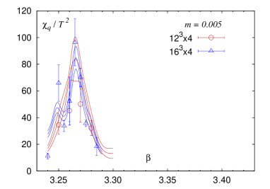
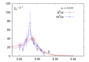
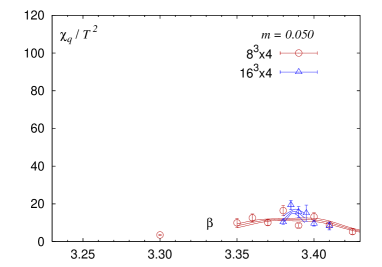
Figure 1: The disconnected part of the chiral susceptibility calculated on $N_{\tau}=4$ lattices at different quark masses.

In agreement with earlier calculations we find that the position of peaks in $\chi_{q}$ and $\chi_{L}$ show only little volume dependence and that the peak height changes only little, although the maxima become somewhat more pronounced on the larger lattices. This is consistent with the transition being a crossover rather than a true phase transition in the infinite volume limit for the range of quark masses explored by us.

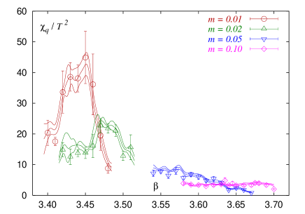
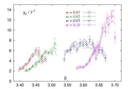
Figure 2: The disconnected part of the chiral susceptibility (left) and the Polyakov loop susceptibility (right) calculated on $16^{3}\times 6$ lattices.

$N_{\tau}$	$m$	$N_{\sigma}$	$\beta_{c,L}$ [from $\chi_{L}$]	$\beta_{c,q}$ [from $\chi_{q}$]	$\beta_{c}$ [averaged]
4	0.100	16	3.4800(27)	3.4804(24)	3.4802(18)
	0.050	16	3.3884(32)	3.3862(47)	3.3877(34)
		8	3.4018(35)	3.3930(201)	3.4015(94)
	0.025	8	3.3294(27)	3.3270(28)	3.3283(31)
	0.010	16	3.2781(7)	3.2781(4)	3.2781(3)
		8	3.2858(71)	3.2820(61)	3.2836(60)
	0.005	16	3.2656(13)	3.2678(12)	3.2667(24)
		12	3.2659(13)	3.2653(12)	3.2656(10)
6	0.200	16	3.8495(11)	3.9015(279)	3.8495(520)
	0.100	16	3.6632(55)	3.6855(105)	3.6680(228)
	0.050	16	3.6076(24)	3.6189(328)	3.6077(115)
	0.020	16	3.4800(110)	3.4800(80)	3.4800(65)
	0.010	16	3.4518(50)	3.4510(83)	3.4516(44)

Table 2: Critical couplings determined from the location of peaks in the Polyakov loop susceptibility as well as in the disconnected parts of the chiral susceptibilities. The last column gives the average of $\beta_{c,L}$ and $\beta_{c,q}$ with combined statistical and systematic errors.

IV Zero temperature calculations and the transition temperature

In order to determine the transition temperature in units of some physical quantity we performed zero temperature calculations on $16^{3}\times 32$ lattices in the vicinity of the pseudo-critical coupling $\beta_{c}$. The parameters of these calculations together with the accumulated statistics are summarized in Table 3. We have calculated the static quark potential and meson correlators on each 10th trajectory generated.

The static potential has been calculated using the ratios of the Wilson loops at two neighboring time-slices and extrapolating them to infinite time separation with the help of constant plus exponential form. The spatial transporters in the Wilson loop have been constructed from spatially smeared links with APE smearing. The weight of the 3 link staple was $\gamma=0.4$ and we used ten steps of APE smearing. From the static potential we have determined the string tension and the Sommer parameter $r_{0}$ defined as Sommer

$$r^{2}\frac{{\rm d}V_{\bar{q}q}(r)}{{\rm d}r}\biggl{|}_{r=r_{0}}=1.65.$$ (5)

When extracting $r_{0}$ and the string tension on coarse lattices, such as the ones used in thermodynamics studies, the violation of rotational symmetry has to be taken into account. We do this using the procedure described in detail in our recent paper us . The value of Sommer scale and the string tension are given in Table 3 for different quark masses. Having determined $r_{0}$ for different gauge couplings and quark masses allows us to perform interpolations of $r_{0}/a$ in these parameters. As in Ref. us we use the following renormalization group inspired interpolation ansatz allton

$$(r_{0}/a)^{-1}=R(\beta)(1+B\hat{a}^{2}(\beta)+C\hat{a}^{4}(\beta)){\rm e}^{A(2m_{l}+m_{s})+D}\;.$$ (6)

Here $R(\beta)$ is 2-loop beta function of 3 flavor QCD. In the interpolation we also used the values of $r_{0}/a$ determined in our 2+1 flavor study us in addition to those shown in Table 3, giving $A=1.45(5)$, $B=1.20(17)$, $C=0.21(6)$ and $D=2.41(5)$ with $\chi^{2}/dof=0.9$. This was the reason for using the notation $m_{l}$ and $m_{s}$ for the light and the strange quark mass in Eq. (6) . For 3 degenerate flavors of course $m_{s}=m_{l}=m$. In Table 3 we also show the values of $r_{0}/a$ obtained from this ansatz for each of the parameter sets.

Meson masses have been calculated using the four local staggered meson operators. We used point-wall meson correlation functions with a $Z_{2}$ wall source. To extract the meson masses from the correlation functions we used a double exponential ansatz which takes into account the two lowest states with opposite parity. The two lowest pseudo-scalar meson masses as well as the lightest vector meson mass are shown in Table 3. The breaking of the flavor symmetry can be quantified by the quadratic splitting of the pseudo-scalar masses: $\Delta_{ps}=(m_{ps2}^{2}-m_{ps}^{2})r_{0}^{2}$, where $m_{ps2}$ is the mass of the lightest pseudo-scalar non-Goldstone meson that is present with staggered fermions. This quantity should be quark mass independent for sufficiently small quark masses and should vanish as ${\cal O}(a^{2})$ when the continuum limit ( $a\rightarrow 0$) is approached. In the last column of Table 3 we show the value of $\Delta_{ps}$ from our scale setting run for $N_{\tau}=4$ and $N_{\tau}=6$. As we see from the table this quantity does not decrease quite as fast as $a^{2}$. This is an indication that on the coarse lattice, corrections to asymptotic scaling are still important.

$\beta$	$m$	# traj	$m_{ps}$	$m_{ps2}$	$m_{V}$	$r_{0}$	$(r_{0})_{smooth}$	$\sqrt{\sigma}$	$\Delta_{ps}$
3.3877	0.050	7800	0.7084(1)	1.094(7)	1.310(20)	2.066(7)[7]	2.061	0.552(12)[12]	2.97(7)
3.3270	0.025	12000	0.5118(3)	0.998(24)	1.222(32)	1.982(14)[13]	1.989	0.564(11)[11]	2.90(20)
3.2680	0.005	1500	0.2341(9)	0.860(90)	1.250(50)	1.888(15)[9]	1.888	0.587(17)[17]	2.44(55)
3.46345	0.020	4420	0.4413(8)	0.665(5)	0.908(11)	2.797(20)[20]	2.813	0.404(6)[6]	1.94(9)
3.4400	0.010	4290	0.3210(7)	0.594(7)	0.882(20)	2.770(13)[13]	2.779	0.405(6)[6]	1.92(7)

Table 3: Parameters of the zero temperature simulations, meson masses, the Sommer scale $r_{0}$ and the string tension. Also shown is the value of $r_{0}$ obtained from the interpolation formula (6). The upper part of the table refers to scale setting runs for our $N_{\tau}=4$ lattices while the lower part to our $N_{\tau}=6$ calculations. In the last column the splitting between the lightest non-Goldstone and the Goldstone pseudo-scalar meson masses squared is shown. All dimensionfull quantities are given in units of the lattice spacings.

With the help of the interpolation formula we can calculate the lattice spacing in units of $r_{0}$ and thus $r_{0}T_{c}$ for different pseudo-scalar meson masses, which is shown in Fig. 3. The error in $a(\beta_{c})$ results in an error in the value of $r_{0}T_{c}$ which is shown in Fig. 3 as thin error-bars. The uncertainty in $\beta_{c}$ itself also contribute to the uncertainty in $r_{0}T_{c}$, which is shown as a thick error-bar in the figure.

If there is a critical point in the $(m,T)$-plane, then universality dictates that $T_{c}(m)-T_{c}(m^{e})\sim(m-m^{e})^{1/(\delta\beta)}$ with $\beta$ and $\delta$ being critical exponents. In the case of three degenerate flavors the line of the 1st order transition in the $(m,T)$ plane ends in a critical end-point $m_{e},T_{c}(m^{e})$ belonging to the Z(2) universality class. For this universality class we have $\delta\beta=1.5654$. Therefore we attempted a combined continuum and chiral extrapolation using the following extrapolation ansatz

$$r_{0}T_{c}(m_{ps},N_{\tau})=r_{0}T_{c}|_{cont}(m_{ps}^{e})+A\left(\left(r_{0}m_{ps}\right)^{2}-\left(r_{0}m_{ps,c}\right)^{2}\right)^{1/(\delta\beta)}+B/N_{\tau}^{2}.$$ (7)

The value of the quark mass where the transition changes from 1st order to crossover, i.e. the mass corresponding to the end-point, has been estimated in karschlat03 using $N_{\tau}=4$ lattices to be $m^{e}=0.0007(4)$. This translates into the value of the pseudo-scalar mass

$$r_{0}m_{ps}^{e}=0.16^{+3}_{-5}.$$ (8)

It turns out that this large uncertainty in the value of $m_{ps}^{e}$ produces an uncertainty in the extrapolated value of $T_{c}(m_{ps}^{2})$ which is much smaller than the statistical errors. The extrapolation according to Eq. (7) yields

$$r_{0}T_{c}(m_{ps}^{e})=0.429(8),~{}~{}\frac{T_{c}(m_{ps}^{e})}{\sqrt{\sigma}}=0.391(9).$$ (9)

For the fit to $r_{0}T_{c}$ data we get $\chi^{2}/dof=0.7$, while for the fit to $T_{c}(m_{ps}^{e})/\sqrt{\sigma}$ data we have $\chi^{2}/dof=0.4$. The quark mass dependence of the transition temperature is described by Eq. (7) only for $m>m^{e}$. For smaller quark masses the transition is first order and $T_{c}$ depends linearly on the quark mass, i.e. we expect $T_{c}(m_{ps},N_{\tau})=T_{c}|_{cont}^{chiral}+Am_{ps}^{2}+B/N_{\tau}^{2}$. If we would insist on the linear dependence of the transition temperature on the quark mass in the entire mass range, the combined chiral and continuum extrapolation would give

$$r_{0}T_{c}=0.419(9),~{}~{}\frac{T_{c}}{\sqrt{\sigma}}=0.383(10).$$ (10)

The $\chi^{2}/dof$ we have found for this fit is almost the same as for the one above. The value of $T_{c}/\sqrt{\sigma}$ is slightly smaller than the estimate of Ref. karsch01 based on $N_{\tau}=4$ lattice and larger quark masses. This is due to the continuum extrapolation performed in the present work. Note, however, that the value $T_{c}(0)^{N_{t}=4}/\sqrt{\sigma}=0.417(9)$ is entirely consistent with Ref. karsch01 . The value of $T_{c}$ could be compared with the corresponding $2+1$ flavor value $T_{c}r_{0}=0.444(6)[+12][-6]$ in the limit of vanishing $u$ and $d$ quark masses but fixed physical value of $m_{s}$ us . Thus the flavor dependence of $r_{0}T_{c}$ is about or smaller than $5\%$. One should also note that the difference between the transition temperature calculated on $N_{\tau}=4$ and $N_{\tau}=6$ lattices is very similar to that found in 2+1 flavor case us .

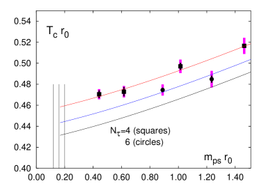
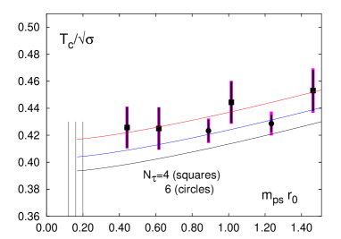
Figure 3: The value of the transition temperature in units of $r_{0}$ (left) and in units of $\sqrt{\sigma}$ (right) calculated on $N_{\tau}=4$ and $N_{\tau}=6$ lattices as function of $m_{ps}$ together with continuum extrapolated value. The vertical line and band indicates the value of $m_{ps}$ where the transition becomes 1st order.

In Ref. karsch01 the transition temperature in the chiral limit has also been estimated in units of the vector mass. Our estimate for $T_{c}/m_{V}|_{m=0}$ is consistent with that result.

V Comparison of R and RHMC algorithm

We investigated the effect of the finite step-size errors of the R algorithm on the properties of the finite temperature transition. We performed calculations on $8^{3}\times 4$ lattices using the p4fat3 action as well as the p4fat7 action and the later will be described in Appendix A in more detail. In the calculations with the p4fat3 action we used a quark mass of $m=0.01$, while in case of p4fat7 action we used two quark masses $m=0.1$ and $0.035$. In our calculations with the R algorithm the step-size of the molecular dynamics evolution was set to be $dt=m/2.5$. Some additional calculations have been done at twice smaller step-size $dt=m/5$. We have calculated the chiral condensate and the Polyakov loop and determined the pseudo-critical couplings which are summarized in Table 4. In Fig. 4 we compare the chiral condensate susceptibility calculated using the R-algorithm and RHMC algorithm for the p4fat3 action. We find that for the p4fat3 action the results obtained with R and RHMC algorithms are identical within statistical errors.

The situation is different for p4fat7. In Fig. 5 the expectation value of the Polyakov loop and the chiral condensate calculated with the two algorithms are shown for two values of the quark mass. Here we see significant differences in the value of the chiral condensate and Polyakov loops calculated with the R algorithm and step-size $dt=m/2.5$ and the corresponding result obtained with RHMC algorithm. We see also a small but statistically significant difference in the value of the pseudo-critical coupling calculated with the two algorithms, c.f. Table 4. The difference becomes much less visible when the step-size is decreased to $dt=m/5$. Figure 5 also suggests that the difference between the results of the two algorithms becomes larger for the smaller quark mass.

Figure 4: The comparison of the disconnected part of chiral condensate susceptibility calculated with the R and RHMC algorithms for p4fat3 with $m=0.01$.

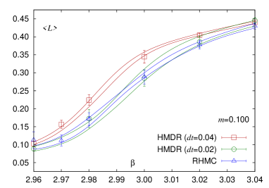
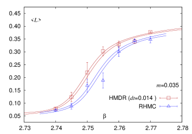
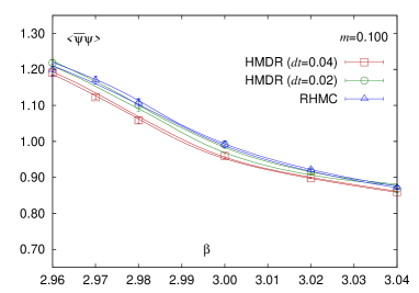
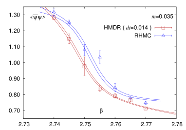
Figure 5: The Polyakov loops (upper part) and the chiral condensate (lower part) calculated with RHMC and R algorithms for the p4fat7 action with $m=0.1$ and $m=0.035$.

For the p4fat7 action we also performed a zero temperature calculation on $16^{3}\times 32$ lattices using the RHMC algorithm to determine the scale. We have calculated meson masses as well the static quark potential. From the later we have extracted $r_{0}$. The results of these calculations are also given in Table 4. Now we can estimate the transition temperature in units of $r_{0}$ for $m=0.035$ calculated with the two algorithms. For the R-algorithm we get $r_{0}T_{c}=0.542(3)$ while for the RHMC algorithm we have $r_{0}T_{c}=0.552(3)$. Thus in the case of the p4fat7 action the R algorithm underestimates the transition temperature roughly by $2\%$.

Action	$m$	Algorithm	$\beta_{c,L}$	$\beta_{c,q}$	$m_{ps}$	$r_{0}/a$
p4fat3	0.010	HMDR	3.2858(71)	3.2820(61)
		RHMC	3.2820(11)	3.2820(11)
p4fat7	0.100	HMDR	2.9850(25)	2.9753(53)
		RHMC	2.9939(33)	2.9831(20)
p4fat7	0.035	HMDR	2.7514(6)	2.7485(7)	0.7884(5)	2.1661(123)
		RHMC	2.7540(6)	2.7515(7)	0.7897(7)	2.2063(108)

Table 4: Comparison of the R and the RHMC algorithms for the pseudo-critical couplings and the scale at the transition temperature.

VI Conclusions

In this paper we have studied the phase transition in 3 flavor QCD at finite temperature using $N_{\tau}=4$ and $N_{\tau}=6$ lattices. For the quark mass corresponding to the second order end-point we find the critical temperature to be $r_{0}T_{c}=0.429(8)$. The transition temperature in the chiral limit is about $2\%$ smaller than the above value. For a given pseudo-scalar meson mass the difference between the transition temperature in 3 flavor and 2+1 flavor case is less than $5\%$. We also find that the cut-off dependence of the transition temperature in 3 and 2+1 flavor QCD is very similar. Furthermore, we find that finite step-size errors present in the R algorithm are negligible, at least for the p4fat3 action at the quark masses studied.

Appendix A

In this appendix we are going to discuss the properties of the finite temperature transition in the case of the p4fat7 action and compare it to the p4fat3 case. In general the gauge transporter in the 1-link term of the p4 action can be replaced by combination of the link variable and different staples, called the fat link, without changing the naive continuum limit. This is true provided the coefficient of different terms in the fat link satisfy appropriate normalization conditions. For example in the case of the fat link with the three link staple only, this condition reads $c_{1}+6c_{3}=1$. Introducing five and seven link staples in addition to the three link staples give the so-called fat7 link kostas . In this case the normalization condition reads: $c_{1}+6c_{3}+24c_{5}+48c_{7}=1$. It is possible to eliminate the leading order coupling to the high momentum gluons with momenta $(0,\pi,0,0)$, $(0,\pi,\pi,0)$ and $(0,\pi,\pi,\pi)$, i.e. to suppress the flavor changing interaction at order $g^{2}a^{2}$ if the coefficients are chosen as kostas

$$\frac{c_{3}}{c_{1}}=\frac{1}{2},~{}\frac{c_{5}}{c_{1}}=\frac{1}{8},~{}\frac{c_{7}}{c_{1}}=\frac{1}{48}.$$ (11)

This gives then the value $c_{1}=-1/8$ for the coefficient of the 1- link term to get the naive continuum limit.

In Fig. 6 we show the chiral condensate calculated on the $N_{\tau}=4$ and $N_{\tau}=6$ lattices. We can see that for small quark masses the transition becomes strongly first order. The value of the chiral condensate in the low temperature phase is also much larger than for the p4fat3 action discussed in the main text. For the smallest quark mass the discontinuity in the chiral condensate is about the same for $N_{\tau}=4$ and $N_{\tau}=6$ lattice, although we would expect it to decrease by roughly a factor of $(6/4)^{3}\simeq 3$ when going from $N_{\tau}=4$ to $N_{\tau}=6$. This could mean that we are dealing with a bulk transition. In Fig. 7 we also compare the pseudo-critical couplings for the p4fat3 and p4fat7 actions. We see that for large quark masses the $N_{\tau}$ dependence of the pseudo-critical coupling is similar, though their values are significantly different. For small quark masses the pseudo-critical couplings calculated for $N_{\tau}=4$ and $6$ come very close together, again suggesting that the transition may be a bulk transition. We did calculations also on $8^{4}$ lattice at $m=0.01$. In Fig. 7 we compare the chiral condensate calculated on $8^{3}\times 4$, $16^{3}\times 6$ and $8^{4}$ lattices. We see a sharp drop in the value of the chiral condensate, which occurs at the same $\beta_{c}$ for $N_{\tau}=6$ and $8$. This again indicates a bulk transition.

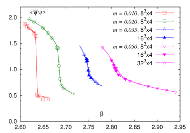
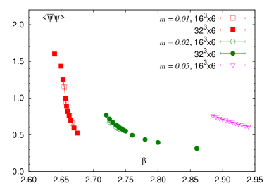
Figure 6: The chiral condensate calculated on $N_{\tau}=4$ (left) and $N_{\tau}=6$ (right) lattices for p4fat7 action.

One may wonder which feature of the p4fat7 action is responsible for the bulk transition. The main difference of the p4fat7 action compared to p4fat3 action as well as to other fat link action (e.g. ASQTAD) is the negative sign of the one link term. Close to the continuum limit the normalization condition $c_{1}+6c_{3}+24c_{5}+48c_{7}=1$ should insure that the combination of 1-, 3-, 5- and 7-link terms will describe a conventionally normalized, positive Dirac kinetic energy. However, at stronger coupling where the gauge field are more disordered, the staples with many links are expected to give a significantly smaller contribution and the 1-link term may dominate, resulting in an effective kinetic energy term with a possibly negative sign. While this would simply correspond to non-standard sign and normalization conventions for the Dirac kinetic energy, it raises the possibility that this effective kinetic energy term will change sign as one passes from strong to weak coupling. Such a sign change could induce a bulk transition. In addition, the change in magnitude of the coefficient in the effective kinetic energy (small for strong coupling and large for weak coupling) would appear reversed in the chiral condensate (large for strong coupling and small for weak coupling) consistent with the observed behavior. To verify this we did calculations with p4fat7 action but with different coefficients which we call the p4fat7’ action. The coefficients were chosen to be

$$c_{1}=\frac{3}{4}\cdot\frac{1}{8},~{}\frac{c_{3}}{c_{1}}=\frac{1}{2},~{}\frac{c_{5}}{c_{1}}=\frac{1}{8},~{}\frac{c_{7}}{c_{1}}=\frac{1}{48}.$$ (12)

For this action we found no evidence for a strong first order transition but only a crossover. This can be seen for example in the behavior of the chiral condensate shown in Fig. 8. Both the value of the chiral condensate and the location of the transition point is very similar to that of the p4fat3 action.

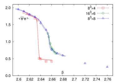
Figure 7: The pseudo-critical couplings for the p4fat3 and p4fat7 actions (left) and the chiral condensate calculated with the p4fat7 action on $8^{3}\times 4$, $16^{3}\times 6$ and $8^{4}$ lattices at $m=0.01$ (right).

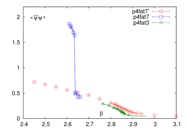
Figure 8: The chiral condensate (left) and its susceptibility (right) for the p4fat7’ action calculated on $8^{3}\times 4$ lattice at $m=0.01$. We also show the chiral condensate calculated with p4fat7 and p4fat3 actions at the same quark mass. The data points for p4fat3 action have been shifted horizontally by $\Delta\beta=-0.437$ for better visibility. The band in the right figure corresponds to Ferrenberg Swendsen re-weighting.

We also calculated the eigenvalues $\lambda=\imath\lambda^{\prime}+2m$ of the p4fat7 Dirac operator. The normalized distribution of the lowest 50 eigenvalues $\lambda^{\prime}$ is shown in Figs. 9 and 10 for the quark masses $m=0.1$ and $m=0.01$, respectively. We have used 100 configurations for $m=0.01$, and 200 configurations for $m=0.1$. Given the above definition of $\lambda^{\prime}$ the breaking of the chiral symmetry manifests itself in a non-zero density at $\lambda^{\prime}\simeq 0$. In Fig. 9 we show the eigenvalue distribution for the larger quark mass $m=0.1$. It shows the expected features: large density of eigenvalues near $\lambda\simeq 0$ in the low temperature phase ($\beta=2.96$), significant drop of eigenvalue density around zero at the transition ($\beta=3.0$) and zero density of eigenvalues at the origin for the deconfined phase ($\beta=3.04$). The situation is different for the smallest quark mass $m=0.01$, where we see non-zero density of eigenvalues at $\lambda\simeq 0$ even in the deconfined phase ($\beta=2.66$). The large decrease in the density of eigenvalues at the origin when going from the confined phase ($\beta=2.635$) to the deconfined explains the large drop in the value of the chiral condensate.

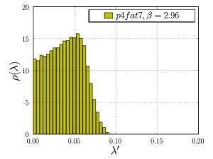
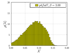
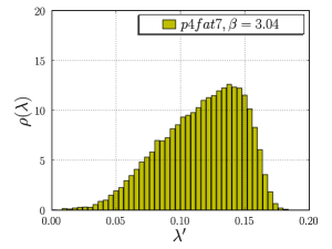
Figure 9: The eigenvalue distributions of the p4fat7 Dirac operator for $m=0.1$ calculated on $8^{3}\times 4$ lattice in the confined phase ($\beta=2.96$), at the transition ($\beta=3.00$) and in the deconfined phase ($\beta=3.04$).

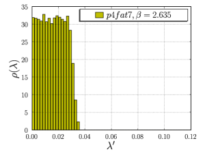
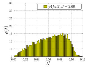
Figure 10: The eigenvalue distributions of the p4fat7 Dirac operator for $m=0.01$ calculated on $8^{3}\times 4$ lattice in the confined phase ($\beta=2.635$), at the transition ($\beta=2.64$) and in the deconfined phase ($\beta=2.66$).

Appendix B

In this appendix we discuss the calculations of the largest and the smallest eigenvalue of the staggered Dirac operator in the free field limit. Let us start our discussion with case of the standard staggered fermions. The free-field staggered Dirac operator acting on a single-component fermion field is given by

$$\mathcal{M}\chi(x)=\sum_{\mu}\eta_{\mu}(x)\left(\chi(x+\mu)-\chi(x-\mu)\right)+2m\chi(x),$$ (13)

where $\eta_{\mu}(x)=(-1)^{x_{0}+x_{1}+\ldots x_{\mu-1}}$ are the normal staggered phases. Consider $\mathcal{M}$ acting on a momentum eigenstate

$$\chi(x) = \chi(p)\,\mathrm{e}^{\imath p\cdot x},$$ (14)

$$\mathcal{M}\chi(x) = \sum_{\mu}\left[\chi(p)\,\mathrm{e}^{\imath p\cdot x}\,(\mathrm{e}^{\imath p_{\mu}}-\mathrm{e}^{-\imath p_{\mu}})\,\mathrm{e}^{\pi_{\mu}\cdot x}\right]+2m\,\chi(p)\,\mathrm{e}^{\imath p\cdot x},$$ (15)

where $\pi_{0}=(0,0,0,0),\pi_{1}=(\pi,0,0,0),\pi_{2}=(\pi,\pi,0,0),\ldots$ Thus, the staggered Dirac operator has non-diagonal terms that couple together states at different corners of the Brillouin zone.

In momentum space, we can write the fermion matrix as

$$\mathcal{M}_{p^{\prime},p} = \sum_{\mu}2\imath\sin(p_{\mu})\,\delta_{p^{\prime},p+\pi_{\mu}}+2m\,\delta_{p^{\prime},p}$$ (16)

$$\mathcal{M^{\dagger}}_{p^{\prime\prime},p^{\prime}} = \sum_{\mu}-2\imath\sin(p^{\prime\prime}_{\mu})\,\delta_{p^{\prime\prime}+\pi_{\mu},p^{\prime}}+2m\,\delta_{p^{\prime\prime},p^{\prime}}.$$ (17)

Then, we have for $\mathcal{M}^{\dagger}\mathcal{M}$

$$\mathcal{M^{\dagger}}_{p^{\prime\prime},p^{\prime}}\mathcal{M}_{p^{\prime},p} = 4\sum_{\mu}\sum_{\nu}\sin(p_{\mu})\sin(p^{\prime\prime}_{\nu})\,\delta_{p^{\prime\prime}+\pi_{\nu},p+\pi_{\mu}}+4m^{2}\delta_{p,p^{\prime\prime}}$$ (18)

$$= 4\sum_{\mu}\sum_{\nu}\sin(p_{\mu})\sin(p_{\nu}+(\pi_{\mu})_{\nu}-(\pi_{\nu})_{\nu})\,\delta_{p^{\prime\prime}+\pi_{\nu},p+\pi_{\mu}}+4m^{2}\delta_{p,p^{\prime\prime}}$$ (20)

$$= 4\sum_{\mu}\sum_{\nu<\mu}\sin(p_{\mu})\sin(p_{\nu}+\pi)\,\delta_{p^{\prime\prime},p+\pi_{\mu}-\pi_{\nu}}+$$

$$4\sum_{\mu}\sum_{\nu>\mu}\sin(p_{\mu})\sin(p_{\nu})\,\delta_{p^{\prime\prime},p+\pi_{\mu}-\pi_{\nu}}+$$

$$4\sum_{\mu}\sin^{2}(p_{\mu})\,\delta_{p,p^{\prime\prime}}+4m^{2}\delta_{p,p^{\prime\prime}}.$$

Noticing that $p+\pi_{\mu}-\pi_{\nu}=p+\pi_{\nu}-\pi_{\mu}$ (mod 2$\pi$), and interchanging $\mu$ and $\nu$ labels in the second piece of Eq. (20), we see that all the off-diagonal pieces of $\mathcal{M}^{\dagger}\mathcal{M}$ cancel, and we are left only with the diagonal piece,

$$(\mathcal{M}^{\dagger}\mathcal{M})_{p^{\prime\prime},p}=4\sum_{\mu}\sin^{2}(p_{\mu})\,\delta_{p,p^{\prime\prime}}+4m^{2}\delta_{p,p^{\prime\prime}}.$$ (21)

As expected, we have a hard lower bound on the eigenvalue spectrum of $\lambda^{2}_{min}=4m^{2}$. The upper bound $\lambda^{2}_{max}=16+4m^{2}$ is realized when $p=(\frac{\pi}{2},\frac{\pi}{2},\frac{\pi}{2},\frac{\pi}{2})$.

The situation for free-field p4 fermions is similar, but a little bit more complicated. Here, the p4 Dirac operator is given by

$$\mathcal{M}\chi(x) = 2m\chi(x)+c_{1,0}\sum_{\mu}\eta_{\mu}(x)\left(\chi(x+\mu)-\chi(x-\mu)\right)+{}$$

$$+c_{1,2}\sum_{\mu}\sum_{\nu\neq\mu}\eta_{\mu}(x)\left(\chi(x+\mu+2\nu)+\chi(x+\mu-2\nu)-\chi(x-\mu+2\nu)-\chi(x-\mu-2\nu)\right),$$

where $c_{1,0}=\frac{3}{4}$ and $c_{1,2}=\frac{1}{24}$. Again, we can examine how $\mathcal{M}$ acts on the momentum eigenstate in Eq. (14). As before, we see that we have off-diagonal pieces that come about as a direct result of the presence of staggered phases.

$$\mathcal{M}\chi(x) = \sum_{\mu}\chi(p)\,\mathrm{e}^{\imath(p+\pi_{\mu})\cdot x}\,\imath\,h_{\mu}(p)+2m\,\chi(p)\,\mathrm{e}^{\imath p\cdot x},$$ (23)

$$h_{\mu}(p) = 2c_{1,0}\sin(p_{\mu})+4c_{1,2}\sum_{\nu\neq\mu}\sin(p_{\mu})\cos(2p_{\nu}).$$ (24)

Or, in matrix form,

$$\mathcal{M}_{p^{\prime},p} = \sum_{\mu}\imath h_{\mu}(p)\,\delta_{p^{\prime},p+\pi_{\mu}}+2m\,\delta_{p^{\prime},p}.$$ (25)

Calculating $\mathcal{M}^{\dagger}\mathcal{M}$, we see that the off-diagonal pieces are eliminated in the same way as in the naive staggered case. Thus, we are left with only diagonal terms,

$$(\mathcal{M}^{\dagger}\mathcal{M})_{p^{\prime\prime},p}=\sum_{\mu}h_{\mu}^{2}(p)\,\delta_{p,p^{\prime\prime}}+4m^{2}\delta_{p,p^{\prime\prime}}.$$ (26)

We see that $\lambda^{2}_{min}=4m^{2}$. Finding $\lambda^{2}_{max}$ requires us to maximize the function $\sum h^{2}_{\mu}(p)$. Doing this, we find the maximum when two of the components of $p$ are equal to $\pi/2$ and the other two components are equal to $0$. For example, $p_{max}=(\pi/2,0,\pi/2,0)$. This yields $\lambda^{2}_{max}=50/9+4m^{2}$ for the p4 action. A similar calculation for the Naik action yields $\lambda^{2}_{max}=196/9+4m^{2}$.

For completeness, we also quote the eigenvectors of the free p4 Dirac operator. Using a slightly different method we find,

$$\chi(x)\equiv\chi_{\rho}(X)=\left[\imath\sum_{\mu}\Gamma_{\rho\rho^{\prime}}^{\mu}(p)\,\sin p_{\mu}\left(2c_{1,0}+4c_{1,2}\sum_{\nu\neq\mu}\cos 2p_{\nu}\right)+(\lambda-2m)\,\delta_{\rho\rho^{\prime}}\right]u^{0}_{\rho^{\prime}}\;\mathrm{e}^{\imath 2p\cdot X},$$ (27)

where we implicitly sum over $\rho^{\prime}$. Here we have used hypercube coordinates $X$ and $\rho$, where $X$ labels the hypercube and $\rho$ is the offset within the hypercube, $x=2X+\rho$ with $\rho_{\mu}=0,1$. Furthermore, $\Gamma_{\rho\rho^{\prime}}^{\mu}(p)$ is defined by $\Gamma_{\rho\rho^{\prime}}^{\mu}(p):=\eta_{\mu}(\rho)\;[\delta_{(\rho+\hat{\mu}),\rho^{\prime}}+\delta_{(\rho-\hat{\mu}),\rho^{\prime}}]\mathrm{e}^{\imath p\>(\rho-\rho^{\prime})}$ and $u_{\rho}^{0}$ is a constant vector depending only on $\rho$. Finally, the eigenvalue of the free p4 Dirac operator is

$$\lambda=2m\pm\imath\sqrt{\sum_{\mu}\sin^{2}p_{\mu}\left(2c_{1,0}+4c_{1,2}\sum_{\nu\neq\mu}\cos 2p_{\nu}\right)^{2}}.$$ (28)

References

- (1) F. Karsch, Lect. Notes Phys. 583, 209 (2002)
- (2) E. Laermann and O. Philipsen, Ann. Rev. Nucl. Part. Sci. 53, 163 (2003) P. Petreczky, Nucl. Phys. Proc. Suppl. 140, 78 (2005)
- (3) F. Karsch, et al., Nucl. Phys. Proc. Suppl. 129, 614 (2004)
- (4) C. Schmidt, C. R. Allton, S. Ejiri, S. J. Hands, O. Kaczmarek, F. Karsch and E. Laermann, Nucl. Phys. Proc. Suppl. 119, 517 (2003) [arXiv:hep-lat/0209009]. F. Karsch, E. Laermann and C. Schmidt, Phys. Lett. B 520, 41 (2001)
- (5) P. de Forcrand and O. Philipsen, Nucl. Phys. Proc. Suppl. 129, 521 (2004)
- (6) N.H. Christ and X. Liao, Nucl. Phys. B (Proc. Suppl.) 119, 514 (2003)
- (7) F. Karsch, E. Laermann, A. Peikert, Nucl. Phys. B 605, 579 (2001)
- (8) S. A. Gottlieb, W. Liu, D. Toussaint, R. L. Renken and R. L. Sugar, Phys. Rev. D 35, 2531 (1987)
- (9) I. Horváth, A. D. Kennedy and S. Sint, Nucl. Phys. B 73, 834 (1999); M. A. Clark, A. D. Kennedy and Z. Sroczynski, Nucl. Phys. Proc. Suppl. 140, 835 (2005)
- (10) Y. Aoki, Z. Fodor, S. D. Katz and K. K. Szabo, JHEP 0601, 089 (2006)
- (11) P. de Forcrand and O. Philipsen, arXiv:hep-lat/0607017
- (12) J. B. Kogut and D. K. Sinclair, arXiv:hep-lat/0608017
- (13) M. Cheng et al., Phys. Rev. D 74, 054507 (2006)
- (14) F. Karsch, E. Laermann and A. Peikert, Phys. Lett. B 478, 447 (2000)
- (15) U. M. Heller, F. Karsch and B. Sturm, Phys. Rev. D 60, 114502 (1999)
- (16) T. Blum et al., Phys. Rev. D55, 1133 (1997)
- (17) K. Orginos, D. Toussaint and R. L. Sugar [MILC Collaboration], Phys. Rev. D 60, 054503 (1999)
- (18) S. R. Sharpe, arXiv:hep-lat/0610094
- (19) J. C. Sexton, D.H. Weingarten, Nucl. Phys. B380, 665 (1992)
- (20) R. Sommer, Nucl. Phys. B411 (1994) 839
- (21) C. Allton, Nucl. Phys. B [Proc. Suppl.] 53, 867 (1997)