The order of the quantum chromodynamics transition predicted by the standard model of particle physics

Quantum chromodynamics (QCD) is the theory of the strong interaction, explaining (for example) the binding of three almost massless quarks into a much heavier proton or neutron – and thus most of the mass of the visible Universe. The standard model of particle physics predicts a QCD-related transition that is relevant for the evolution of the early Universe. At low temperatures, the dominant degrees of freedom are colourless bound states of hadrons (such as protons and pions). However, QCD is asymptotically free, meaning that at high energies or temperatures the interaction gets weaker and weaker Gross:1973id ; Politzer:1973fx , causing hadrons to break up. This behaviour underlies the predicted cosmological transition between the low-temperature hadronic phase and a high-temperature quark–gluon plasma phase (for simplicity, we use the word ’phase’ to characterize regions with different dominant degrees of freedom). Despite enormous theoretical effort, the nature of this finite-temperature QCD transition (that is, first-order, second-order or analytic crossover) remains ambiguous. Here we determine the nature of the QCD transition using computationally demanding lattice calculations for physical quark masses. Susceptibilities are extrapolated to vanishing lattice spacing for three physical volumes, the smallest and largest of which differ by a factor of five. This ensures that a true transition should result in a dramatic increase of the susceptibilities.No such behaviour is observed: our finite-size scaling analysis shows that the finite-temperature QCD transition in the hot early Universe was not a real phase transition, but an analytic crossover (involving a rapid change, as opposed to a jump, as the temperature varied). As such, it will be difficult to find experimental evidence of this transition from astronomical observations.

During the evolution of the Universe there were particle-physics-related transitions. Although there are strong indications of an inflationary period, we know little about how it affected possible transitions of our known physical model. To understand the consequences, we need a clear picture about these cosmologically relevant transitions. The Standard Model (SM) of particle physics predicts two such transitions.

One of the SM based transitions occurs at temperatures ($T$) of a few hundred GeV. This transition is responsible for the spontaneous breaking of the electroweak symmetry, which gives the masses of the elementary particles. This transition is also related to the electroweak baryon-number violating processes, which had a major influence on the observed baryon-asymmetry of the Universe. Lattice results have shown that the electroweak transition in the SM is an analytic cross-over Karsch:1996yh ; Kajantie:1996mn ; Csikor:1998eu ; Gurtler:1997hr .

The second transition occurs at $T\approx$200 MeV. It is related to the spontaneous breaking of the chiral symmetry of QCD. The nature of the QCD transition affects our understanding of the Universe’s evolution (see Ref. Schwarz:2003du for example). In a strong first-order phase transition the quark–gluon plasma supercools before bubbles of hadron gas are formed. These bubbles grow, collide and merge, during which gravitational waves could be produced Witten:1984rs . Baryon-enriched nuggets could remain between the bubbles, contributing to dark matter. The hadronic phase is the initial condition for nucleosynthesis, so inhomogeneities in this phase could have a strong effect on nucleosynthesis Applegate:1985qt . As the first-order phase transition weakens, these effects become less pronounced. Our calculations provide strong evidence that the QCD transition is a crossover and thus the above scenarios —and many others— are ruled out.

We emphasize that extensive experimental work is currently being done with heavy ion collisions to study the QCD transition (most recently at the Relativistic Heavy Ion Collider, RHIC). Both for the cosmological transition and for RHIC, the net baryon densities are quite small, and so the baryonic chemical potentials ($\mu$) are much less than the typical hadron masses ($\approx$45 MeV at RHIC and negligible in the early Universe). A calculation at $\mu$=0 is directly applicable for the cosmological transition and most probably also determines the nature of the transition at RHIC. Thus we carry out our analysis at $\mu$=0.

QCD is a generalised version of quantum electrodynamics (QED). The Euclidean Lagrangian with gauge coupling $g$ and with a quark mass of $m$ can be written as ${\cal L}$=$-1/(2g^{2})$Tr$F_{\mu\nu}$$F_{\mu\nu}$+${\bar{\psi}}$$\gamma_{\mu}$($\partial_{\mu}$+$A_{\mu}$+m)$\psi$, where $F_{\mu\nu}$=$\partial_{\mu}$$A_{\nu}$-$\partial_{\nu}$$A_{\mu}$+[$A_{\mu}$,$A_{\nu}$]. In electrodynamics the gauge field $A_{\mu}$ is a simple real field, whereas in QCD it is a 3$\times$3 matrix. Consequently the commutator in $F_{\mu\nu}$ vanishes for QED, but it does not vanish in QCD. The $\psi$ fields also have an additional “colour” index in QCD, which runs from 1 to 3. Different types of quarks are represented by fermionic fields with different masses. The action $S$ is defined as the four-volume integral of ${\cal L}$. The basic quantity we determine is the the partition function $Z$, which is the sum of the Boltzmann factors $\exp(-S)$ for all field configurations. Partial derivatives of $Z$ with respect to the masses give rise to the order parameters we studied here.

There are some QCD results and model calculations to determine the order of the transition at $\mu$=0 and $\mu$$\neq$0 for different fermionic contents (compare refs Pisarski:1983ms ; Celik:1983wz ; Kogut:1982rt ; Gottlieb:1985ug ; Brown:1988qe ; Fukugita:1989yb ; Halasz:1998qr ; Berges:1998rc ; Schaefer:2004en ; Herpay:2005yr ). Unfortunately, none of these approaches can give an unambiguous answer for the order of the transition for physical values of the quark masses. The only known systematic technique which could give a final answer is lattice QCD.

Lattice QCD discretises the above Lagrangian on a four-dimensional lattice and extrapolates the results to vanishing lattice spacing ($a\longrightarrow 0$). A convenient way to carry out this discretisation is to put the fermionic variables on the sites of the lattice, whereas the gauge fields are treated as $3\times 3$ matrices connecting these sites. In this sense, lattice QCD is a classical four-dimensional statistical physics system. One important difference compared to three dimensional systems is that the temperature ($T$) is determined by the additional, Euclidean time extension ($N_{t}$): $T$=1/($N_{t}a$). Keeping the temperature fixed (such as at the transition point) one can reduce $a$ and approach the continuum limit by increasing $N_{t}$ (see Methods).

There are several lattice results for the order of the QCD transition (for the two most popular lattice fermion formulations see refs Brown:1990ev and AliKhan:2000iz ), although they have unknown systematics. We emphasise that from the lattice point of view two ’ingredients’ are necessary to eliminate these systematic uncertainties.

The first ingredient is to use physical values for the quark masses. Owing to the computational costs this is a great challenge in lattice QCD. Previous analyses used computationally less demanding non-physically large quark masses. However, these choices have limited relevance. The order of the transition depends on the quark mass. For example, in three-flavour QCD for vanishing quark masses the transition is of first-order. For intermediate masses it is most probably a crossover. For infinitely heavy quark masses the transition is again first-order. For questions concerning the restoration of chiral symmetry (such as the order of the transition), a controlled extrapolation from larger quark masses (such as chiral perturbation theory) is unavailable, and so the physical quark masses should be used directly.

The second ingredient is to remove the uncertainty associated with the lattice discretization. Discretization errors disappear in the continuum limit; however, they strongly influence the results at non-vanishing lattice spacing. In three-flavour unimproved staggered QCD, using a lattice spacing of about 0.28 fm, the first-order and the crossover regions are separated by a pseudoscalar mass of $m_{\pi,c}$$\approx$300 MeV. Studying the same three-flavour theory with the same lattice spacing, but with an improved p4 action (which has different discretization errors) we obtain $m_{\pi,c}$$\approx$70 MeV. In the first approximation, a pseudoscalar mass of 140 MeV (which corresponds to the numerical value of the physical pion mass) would be in the first-order transition region, whereas using the second approximation, it would be in the crossover region. The different discretisation uncertainties are solely responsible for these qualitatively different results Karsch:2003va . Therefore, the proper approach is to use physical quark masses, and to extrapolate to vanishing lattice spacings. Our work eliminates both of the above uncertainties.

Our goal is to identify the nature of the transition for physical quark masses as we approach the continuum limit. We will study the finite size scaling of the lattice chiral susceptibilities $\chi(N_{s},N_{t})$=$\partial^{2}$/$(\partial$$m_{ud}^{2})$($T/V$)$\cdot\log Z$, where $m_{ud}$ is the mass of the light u,d quarks and $N_{s}$ is the spatial extension. This susceptibility shows a pronounced peak around the transition temperature ($T_{c}$). For a real phase transition the height of the susceptibility peak increases and the width of the peak decreases when we increase the volume. For a first-order phase transition the finite size scaling is determined by the geometric dimension, the height is proportional to $V$, and the width is proportional to $1/V$. For a second-order transition the singular behaviour is given by some power of $V$, defined by the critical exponents. The picture would be completely different for an analytic crossover. There would be no singular behaviour and the susceptibility peak does not get sharper when we increase the volume; instead, its height and width will be $V$ independent for large volumes.

Figure 1 shows the susceptibilities for the light quarks for $N_{t}=$4 and 6, for which we used aspect ratios $r=N_{s}/N_{t}$ ranging from 3 to 6 and 3 to 5, respectively. A clear signal for an analytic crossover for both lattice spacings can be seen. However, these curves do not say much about the continuum behaviour of the theory. In principle a phenomenon as unfortunate as that in the three-flavour theory could occur Karsch:2003va , in which the reduction of the discretization effects changed the nature of the transition for a pseudoscalar mass of $\approx$140 MeV.

Because we are interested in genuine temperature effects we subtract the $T$=0 susceptibility and study only the difference between $T$$\neq$0 and $T$=0 at different lattice spacings. To do it properly, when we approach the continuum limit the renormalization of $\chi$ has to be performed. This leads to $m^{2}$$\Delta$$\chi$, which we study (see Methods).

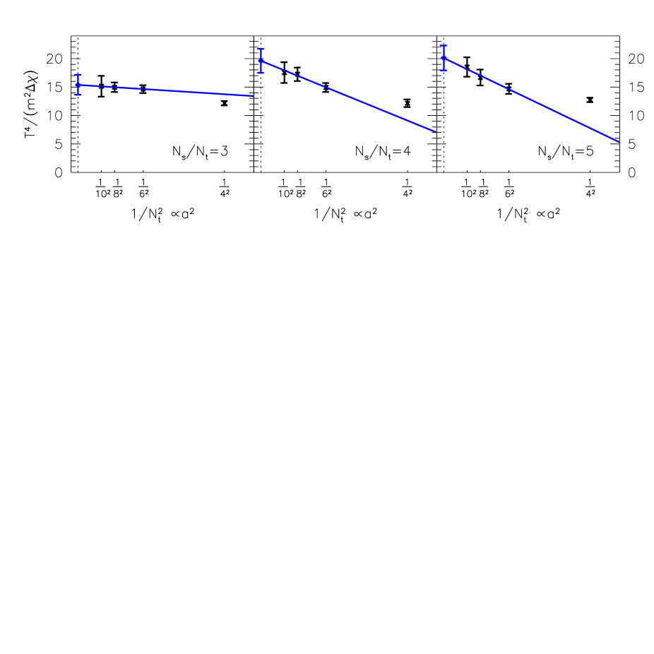
Figure 2: Normalised susceptibilities $T^{4}/(m^{2}\Delta\chi)$ for the light quarks for aspect ratios r=3 (left panel) r=4 (middle panel) and r=5 (right panel) as functions of the lattice spacing. Continuum extrapolations are carried out for all three physical volumes and the results are given by the leftmost blue diamonds. Error bars are s.e.m with systematic estimates.

To give a continuum result for the order of the transition we carry out a finite size scaling analysis of the dimensionless quantity $T^{4}/(m^{2}\Delta\chi)$ directly in the continuum limit. For this study we need the height of the susceptibility peaks in the continuum limit for fixed physical volumes. The continuum extrapolations are done using four different lattice spacings ($N_{t}$=4,6,8 and 10). The volumes at different lattice spacings are fixed in units of $T_{c}$, and thus $VT_{c}^{3}$=$3^{3}$,$4^{3}$ and $5^{3}$ were chosen. (In three cases the computer architecture did not allow us to take the above ratios directly. In these cases, we used the next possible volume and interpolated or extrapolated. The height of the peak depends weakly on the volume, so these procedures were always safe.) Altogether we used twelve different lattice volumes ranging from $4\cdot 12^{3}$ to $10\cdot 48^{3}$ at $T>0$. For the $T=0$ runs lattice volumes from $24\cdot 12^{3}$ up to $56\cdot 28^{3}$ were used. The number of trajectories were between 1500 and 8000 for $T>0$ and between 1500 and 3000 for $T=0$, respectively. Figure 2 shows the continuum extrapolation for the three different physical volumes. The $N_{t}$=4 results are slightly off but the $N_{t}$=6,8 and 10 results show a good $a^{2}$$\propto$$1/N_{t}^{2}$ scaling.

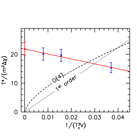
Figure 3: Continuum extrapolated susceptibilities $T^{4}/(m^{2}\Delta\chi)$ as a function of 1/$(T_{c}^{3}V)$. For true phase transitions the infinite volume extrapolation should be consistent with zero, whereas for an analytic crossover the infinite volume extrapolation gives a non-vanishing value. The continuum-extrapolated susceptibilities show no phase-transition-like volume dependence, though the volume changes by a factor of five. The V$\rightarrow$$\infty$ extrapolated value is 22(2) which is 11$\sigma$ away from zero. For illustration, we fit the expected asymptotic behaviour for first-order and O(4) (second order) phase transitions shown by dotted and dashed lines, which results in chance probabilities of $10^{-19}$ ($7\times 10^{-13}$), respectively. Error bars are s.e.m with systematic estimates.

Having obtained the continuum values for $T^{4}/(m^{2}\Delta\chi)$ at fixed physical volumes, we study the finite size scaling of the results. Figure 3 shows our final results. The volume dependence strongly suggests that there is no true phase transition but only an analytic crossover in QCD.

Methods. An introduction to lattice QCD at $T$=0 and $T$$\neq$0 can be found in refs Davies:2002cx and Ukawa:1995tc for example. The detailed form of our Symanzik improved gauge and stout-link improved staggered fermionic action can be found in ref. Aoki:2005vt . (Staggered QCD with $n_{f}$$\neq$4 flavours uses the fourth-root description for the fermionic determinant, the relevance of which is recently intensively discussed, see ref. Bernard:2006ee and references therein.) In this work we also used a stout-smearing level of 2. Note that stout-link improvement makes the staggered fermion taste symmetry violation small even at moderate lattice spacings (for an illustration, see Fig. 1 of ref. Aoki:2005vt ). Taste symmetry violation errors –as with other discretization errors of the staggered formalism– scale as $a^{2}$ and disappear only after extrapolating to the continuum limit. We carried out this extrapolation and explicitly checked that taste symmetry violations for our smallest lattice spacings are already within this $a^{2}$ scaling regime, and so we conclude that the extrapolation is reliable.

In previous staggered analyses the gauge configurations were produced by the R-algorithm Gottlieb:1987mq at a given step size. The step size is an intrinsic parameter of the algorithm, which has to be extrapolated to zero. Instead of using the approximate R-algorithm, we used Aoki:2005vt the exact rational hybrid Monte-Carlo algorithm Clark:2003na in large scale simulations. This technique, which we apply also in this paper, expresses the fractional powers of the Dirac operator by rational functions.

In our simulations we approach the continuum limit along the line of constant physics (LCP). The LCP is defined by relationships between the bare lattice parameters (gauge coupling $g$ and lattice bare quark masses for light quarks $m_{ud}$ and strange quark $m_{s}$). These relationships ensure that the physics (such as ratios of physical observables) remain constant, while changing any of the parameters. We note that the LCP is unambiguous (independent of the physical quantities, which are used to define the above relationships) only in the vicinity of the continuum limit. The present work uses the LCP defined by fixing two ratios to their physical values: $m_{K}$/$m_{\pi}$=3.689 and $f_{K}$/$m_{\pi}$=1.185 ($m_{K}$ is the mass of the kaon, $f_{K}$ is its decay constant and $m_{\pi}$ is the mass of the pion). Figure 4 shows the LCP used in this work.

Using the above action, simulation algorithm and parameter set based on our LCP, we performed simulations at $T$$\neq$0 and $T$=0. At $T$$\neq$0 we always used the physical quark masses at four different temporal extensions: $N_{t}$=4,6,8 and 10 lattices. The aspect ratios ($N_{s}$/$N_{t}$) were taken to be 3,4 and 5 (for the $N_{t}=4$ case also 6), which results in a factor-of-8 change in the volume ($V$). In the chirally broken phase (our zero temperature simulations always belong to this class) chiral perturbation theory can be used to extrapolate to the physical values of the light quark masses in a controlled manner. Therefore we used four pion masses ($m_{\pi}\approx$235, 300, 355 and 405 MeV), which are somewhat larger than the physical one. The spatial extension was chosen to ensure $N_{s}$$m_{\pi}$$>$$\sim$4. The computational requirement for the present work was 0.8 teraflopyears.

The renormalization of the chiral susceptibility can be done by taking the second derivative of the free energy density ($f$) with respect to the renormalized mass ($m_{r}$). We apply the usual definition: $f/T^{4}=-N_{t}^{4}[\log Z(N_{s},N_{t})/(N_{t}N_{s}^{3})-\log Z(N_{s0},N_{t0})/(N_{t0}N_{s0}^{3})]$. This quantity has a correct continuum limit. The subtraction term is obtained at $T$=0, for which simulations are carried out on lattices with $N_{s0}$, $N_{t0}$ spatial and temporal extensions (otherwise at the same parameters of the action). The bare light quark mass is related to $m_{r}$ by the mass renormalisation constant $m_{r}$=$Z_{m}$$\cdot$$m_{ud}$. Note that $Z_{m}$ falls out of the combination $m_{r}^{2}$$\partial^{2}$/$\partial$$m_{r}^{2}$=$m_{ud}^{2}$$\partial^{2}$/$\partial$$m_{ud}^{2}$. Thus, $m_{ud}^{2}\left[\chi(N_{s},N_{t})-\chi(N_{s0},N_{t0})\right]$ also has a continuum limit (for its maximum values for different $N_{t}$, and in the continuum limit we use the shorthand notation $m^{2}$$\Delta\chi$). For the subtraction, $T$=0 simulations are performed and chiral perturbation theory is applied.

Acknowledgements We thank F. Csikor, A. Dougall, K.-H. Kampert, M. Nagy, Z. Rácz and D.J. Schwarz for discussions. This research was partially supported by a DFG German Science Grant, OTKA Hungarian Science Grants and an EU research grant. The computations were carried out on PC clusters at the University of Budapest and Wuppertal with next-neighbour communication architecture Fodor:2002zi and on the BlueGene/L machine in Jülich. A modified version of the publicly available MILC code (http://physics.indiana.edu/$\tilde{\ }$sg/milc.html) was used.

Figures

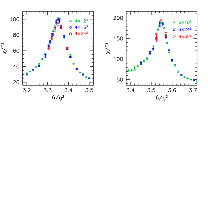
Figure 1: Susceptibilities for the light quarks for $N_{t}$=4 (left panel) and for $N_{t}$=6 (right panel) as a function of $6/g^{2}$, where $g$ is the gauge coupling ($T$ grows with $6/g^{2}$). The largest volume is eight times bigger than the smallest one, so a first-order phase transition would predict a susceptibility peak that is eight times higher (for a second-order phase transition the increase would be somewhat less, but still dramatic). Instead of such a significant change we do not observe any volume dependence. Error bars are s.e.m.

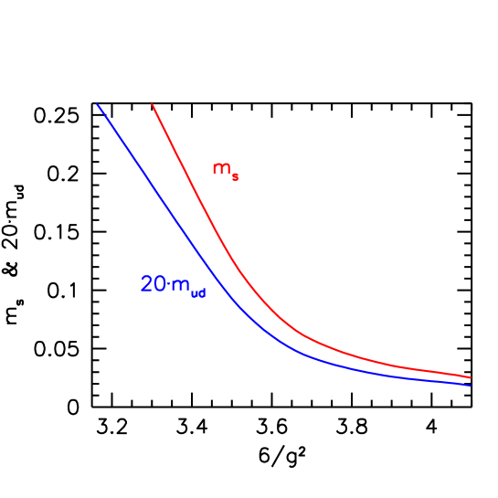
Figure 4: The line of constant physics. We show our choice for $m_{s}$ (strange quark mass) and 20$m_{ud}$ (u,d quark masses) in lattice units as functions of $6/g^{2}$.

References

- [1] D. J. Gross and Frank Wilczek. Ultraviolet behavior of non-abelian gauge theories. Phys. Rev. Lett., 30:1343–1346, 1973.
- [2] H. David Politzer. Reliable perturbative results for strong interactions? Phys. Rev. Lett., 30:1346–1349, 1973.
- [3] F. Karsch, T. Neuhaus, A. Patkos, and J. Rank. Critical higgs mass and temperature dependence of gauge boson masses in the su(2) gauge-higgs model. Nucl. Phys. Proc. Suppl., 53:623–625, 1997.
- [4] K. Kajantie, M. Laine, K. Rummukainen, and Mikhail E. Shaposhnikov. Is there a hot electroweak phase transition at ? Phys. Rev. Lett., 77:2887–2890, 1996.
- [5] F. Csikor, Z. Fodor, and J. Heitger. Endpoint of the hot electroweak phase transition. Phys. Rev. Lett., 82:21–24, 1999.
- [6] M. Gurtler, Ernst-Michael Ilgenfritz, and A. Schiller. Where the electroweak phase transition ends. Phys. Rev., D56:3888–3895, 1997.
- [7] Dominik J. Schwarz. The first second of the universe. Annalen Phys., 12:220–270, 2003.
- [8] Edward Witten. Cosmic separation of phases. Phys. Rev., D30:272–285, 1984.
- [9] J. H. Applegate and C. J. Hogan. Relics of cosmic quark condensation. Phys. Rev., D31:3037–3045, 1985.
- [10] Robert D. Pisarski and Frank Wilczek. Remarks on the chiral phase transition in chromodynamics. Phys. Rev., D29:338–341, 1984.
- [11] T. Celik, J. Engels, and H. Satz. The order of the deconfinement transition in su(3) yang- mills theory. Phys. Lett., B125:411–414, 1983.
- [12] John B. Kogut et al. Deconfinement and chiral symmetry restoration at finite temperatures in su(2) and su(3) gauge theories. Phys. Rev. Lett., 50:393–396, 1983.
- [13] Steven A. Gottlieb et al. The deconfining phase transition and the continuum limit of lattice quantum chromodynamics. Phys. Rev. Lett., 55:1958–1961, 1985.
- [14] F. R. Brown, N. H. Christ, Y. F. Deng, M. S. Gao, and T. J. Woch. Nature of the deconfining phase transition in su(3) lattice gauge theory. Phys. Rev. Lett., 61:2058–2061, 1988.
- [15] M. Fukugita, M. Okawa, and A. Ukawa. Order of the deconfining phase transition in su(3) lattice gauge theory. Phys. Rev. Lett., 63:1768–1771, 1989.
- [16] M. A. Halasz, A. D. Jackson, R. E. Shrock, Misha A. Stephanov, and J. J. M. Verbaarschot. On the phase diagram of QCD. Phys. Rev., D58:096007 [11 pages], 1998.
- [17] Jurgen Berges and Krishna Rajagopal. Color superconductivity and chiral symmetry restoration at nonzero baryon density and temperature. Nucl. Phys., B538:215–232, 1999.
- [18] Bernd-Jochen Schaefer and Jochen Wambach. The phase diagram of the quark meson model. Nucl. Phys., A757:479–492, 2005.
- [19] T. Herpay, A. Patkos, Zs. Szep, and P. Szepfalusy. Mapping the boundary of the first order finite temperature restoration of chiral symmetry in the (m(pi) - m(k))-plane with a linear sigma model. Phys. Rev., D71:125017 [15 pages], 2005.
- [20] Frank R. Brown et al. On the existence of a phase transition for qcd with three light quarks. Phys. Rev. Lett., 65:2491–2494, 1990.
- [21] A. Ali Khan et al. Phase structure and critical temperature of two flavor qcd with renormalization group improved gauge action and clover improved wilson quark action. Phys. Rev., D63:034502 [11 pages], 2001.
- [22] F. Karsch et al. Where is the chiral critical point in 3-flavor qcd? Nucl. Phys. Proc. Suppl., 129:614–616, 2004.
- [23] Christine Davies. Lattice qcd. (unpublished), 2002.
- [24] Akira Ukawa. Lectures on lattice qcd at finite temperature. (unpublished). Talk given at Uehling Summer School on Phenomenology and Lattice QCD, Seattle, WA, 21 Jun - 2 Jul 1993.
- [25] Y. Aoki, Z. Fodor, S. D. Katz, and K. K. Szabo. The equation of state in lattice qcd: With physical quark masses towards the continuum limit. JHEP, 01:089 [16 pages], 2006.
- [26] Claude Bernard, Maarten Golterman, and Yigal Shamir. Observations on staggered fermions at non-zero lattice spacing. Phys. Rev., D73:114511 [10 pages], 2006.
- [27] Steven A. Gottlieb, W. Liu, D. Toussaint, R. L. Renken, and R. L. Sugar. Hybrid molecular dynamics algorithms for the numerical simulation of quantum chromodynamics. Phys. Rev., D35:2531–2542, 1987.
- [28] M. A. Clark and A. D. Kennedy. The rhmc algorithm for 2 flavors of dynamical staggered fermions. Nucl. Phys. Proc. Suppl., 129:850–852, 2004.
- [29] Zoltan Fodor, Sandor D. Katz, and Gabor Papp. Better than $1/mflops sustained: A scalable pc-based parallel computer for lattice qcd. Comput. Phys. Commun., 152:121–134, 2003.