Electromagnetic Corrections in Partially Quenched Chiral Perturbation Theory

Abstract

We introduce photons in Partially Quenched Chiral Perturbation Theory and calculate the resulting electromagnetic loop-corrections at NLO for the charged meson masses and decay constants. We also present a numerical analysis to indicate the size of the different corrections. We show that several phenomenologically relevant quantities can be calculated consistently with photons which couple only to the valence quarks, allowing the use of gluon configurations produced without dynamical photons.

I Introduction

This is the sixth paper in a series of studies of Partial Quenching (PQ) in Chiral Perturbation Theory ($\chi$PT) Weinberg ; GL1 ; GL2 , where we now investigate the effects of including electromagnetic loop corrections in the theory. The motivation for using partial quenching in $\chi$PT (and indeed for studying $\chi$PT itself) comes from the fact that even though quantum chromodynamics (QCD) over time has become the generally accepted theory of the strong interaction, it has still proven difficult to use this theory to derive low-energy hadronic observables such as masses and decay constants.

An alternative approach is to use Lattice QCD simulations to this end. Computational limitations have however hindered such simulations for light particles since they can propagate over large distances, requiring very large lattice sizes. Because of this, most simulations have so far been performed with heavier quark masses than those of the physical world.

On the other hand, Chiral Perturbation Theory provides a theoretically correct description of the low-energy properties of QCD, and can be used to extrapolate the results of lattice simulations down to the masses of the physical regime of QCD. In particular, one can use lattice simulations to determine the low-energy constants of $\chi$PT by fitting $\chi$PT calculations to corresponding lattice simulations, thereby getting estimates of hadronic low-energy observables.

One problem with this approach is that reliable predictions from $\chi$PT require that one keeps the quark masses fairly small, and so far it has proven difficult to reach the chiral regime in the lattice simulations. However, progress is being made on this front. A complementary approach is therefore to use partial quenching where one introduces a separate quark mass for the calculations of closed quark loops, referred to as sea quarks, compared to the quark lines which are connected to external sources, referred to as valence quarks. This has the advantage over full QCD calculations that results with more values of the valence quark masses can be obtained with a smaller number of values of sea quark masses, which is useful since varying the latter is computationally more expensive.

Unquenched QCD may be recovered from partially quenched QCD (PQQCD) by taking the limit of equal sea and valence quark masses, and therefore it follows that QCD and PQQCD are continuously connected by the variation of sea-quark masses. This means that, in contrast to a fully quenched theory where the effects of the closed quark loops are neglected altogether, one can relate partially quenched QCD simulations to the unquenched physical observables of the real world.

Chiral Perturbation Theory has also been extended to include both quenching and partial quenching Morel ; BG1 ; SharpeA ; BG2 . The formulation of Partially Quenched $\chi$PT (PQ$\chi$PT) is such that the dependence on the quark masses is explicit, and thus the limit of equal sea and valence quark masses can also be considered for PQ$\chi$PT. This allows for determination of the physically relevant LECs of $\chi$PT by fits of partially quenched $\chi$PT (PQ$\chi$PT) to partially quenched lattice simulations (PQQCD), see e.g. the discussion in Sharpe1 . In particular, the LECs of $\chi$PT, which are of physical significance, can be obtained directly from those of PQ$\chi$PT. More detailed discussions of this and references to earlier work can be found in the papers of Sharpe and Shoresh Sharpe1 ; Sharpe2 . The calculations in this paper have been performed in three-flavor PQ$\chi$PT without the $\Phi_{0}$ Sharpe2 degree of freedom. In our earlier work with Timo Lähde BDL ; BL1 ; BL2 ; BDL2 ; BD1 we have calculated masses and decay constants for the charged, or off-diagonal, mesons to next-to-next-to-leading-order in PQ$\chi$PT. However, in order to compare with the experimental values at high precision one needs to take electromagnetic effects into account as well.

Electromagnetic corrections in $\chi$PT have a long history. The lowest order (LO) was done by Dashen Dashen . The first corrections to this were worked out in Ref. Langacker . That large corrections might appear was pointed out in Refs. DHW ; BijnensDashen ; Maltman , where these corrections appear both from chiral logarithms and effects persisting at large $N_{c}$. The work in pure $\chi$PT was started by UrechUrech1 and by Neufeld and Rupertsberger Neufeld . The NLO expressions for the masses were calculated in both papers and the decay constants in the second. More recent work on estimating the relevant LECs can be found in Refs. BP ; Moussallam1 ; Donoghue ; Moussallam2 ; Moussallam3 ; Pinzke . Note that there are several subtleties involved in defining electromagnetic corrections at low energies as discussed in Refs. BP ; Moussallam1 ; Gasser with increasing levels of detail. There are also first exploratory lattice QCD calculations Lattice1 ; Lattice2 ; Lattice3 ; Lattice4 .

In this paper we present the extension of PQ$\chi$PT to include dynamical photons to NLO. In addition we calculate the NLO expressions for the masses of the charged, or offdiagonal, mesons with virtual photon-loop corrections for all possible degrees of degeneracy in the valence- and sea-quark masses. We do the same for the decay constants, i.e. we determine the ${\cal O}(e^{2})$ and ${\cal O}(e^{2}p^{2})$ corrections in PQ$\chi$PT to all these quantities.

We point out that the two phenomenologically relevant quantities $\Delta M^{2}$ and $\Delta F$ for differences of masses and decay constants, can be determined from partially quenched lattice calculations where the photons are only coupled to the valence quarks. This has the important consequence that these quantities can be calculated in lattice QCD with gluon configurations generated without dynamical photons.

The paper is organised as follows. First we present the technical background and notation already present in the earlier work BDL ; BL1 ; BL2 ; BDL2 ; BD1 in Sect. II. We also present the results for the needed loop integrals there. The extension to dynamical photons is discussed in Sect. III. Here we give the Lagrangians needed, as well as the subtractions needed to obtain finite results. The analytical expressions for the masses and decay constants are given in Sect. IV and discussed in Sect. V. Some illustrative numerical results are give in Sect. VI and we recapitulate the main conclusions in Sect. VII.

II PQ$\chi$PT, technical overview

Here we give a short overview of the technical aspects of PQ$\chi$PT. A more thorough discussion of the technical aspects of PQ$\chi$PT calculations to NLO (without photons) can be found in Refs. Sharpe1 ; Sharpe2 . Our earlier papers, in particular BDL2 , also contain overviews of the NLO technical and notational details, but the focus there is mainly on the NNLO aspects relevant for those papers. Lectures on standard $\chi$PT can be found in CHPTlectures .

The mechanism which gives different masses to sea quarks and valence quarks in PQ$\chi$PT is introduced by adding explicit sea quarks, as well as unphysical bosonic ghost quarks. The bosonic quarks are needed to cancel all effects of closed loop contributions from valence quarks. This cancellation happens if the masses of the bosonic quarks are set equal to the masses of the valence quarks. The symmetry group of PQ$\chi$PT is essentially given by the graded group

$$G=SU(n_{\mathrm{val}}+n_{\mathrm{sea}}|n_{\mathrm{val}})_{L}\times SU(n_{\mathrm{val}}+n_{\mathrm{sea}}|n_{\mathrm{val}})_{R}\,.$$ (1)

where $n_{\mathrm{val}}$ denotes the number of valence quarks and $n_{\mathrm{sea}}$ the number of sea quarks in the theory. The number of bosonic quarks is by necessity equal to the number of valence quarks. The PQ analog to the field matrix $U$ in ordinary $\chi$PT is given by

$$U\equiv\exp\left(i\sqrt{2}\,\Phi/F_{0}\right)\,.$$ (2)

The matrix $\Phi$ is now a graded matrix, which in terms of a sub-matrix notation for the flavor structure can be written as

$$\Phi=\left(\begin{array}[]{ccc}\Big{[}\;\;q_{V}\bar{q}_{V}\;\;\Big{]}&\Big{[}\;\;q_{V}\bar{q}_{S}\;\;\Big{]}&\Big{[}\;\;q_{V}\bar{q}_{B}\;\;\Big{]}\\ \\ \Big{[}\;\;q_{S}\bar{q}_{V}\;\;\Big{]}&\Big{[}\;\;q_{S}\bar{q}_{S}\;\;\Big{]}&\Big{[}\;\;q_{S}\bar{q}_{B}\;\;\Big{]}\\ \\ \Big{[}\;\;q_{B}\bar{q}_{V}\;\;\Big{]}&\Big{[}\;\;q_{B}\bar{q}_{S}\;\;\Big{]}&\Big{[}\;\;q_{B}\bar{q}_{B}\;\;\Big{]}\end{array}\right)\,.$$ (3)

The brackets denote matrices of the form

$$q_{a}\bar{q}_{b}=\left(\begin{array}[]{ccc}u_{a}\bar{u}_{b}&u_{a}\bar{d}_{b}&u_{a}\bar{s}_{b}\\ d_{a}\bar{u}_{b}&d_{a}\bar{d}_{b}&d_{a}\bar{s}_{b}\\ s_{a}\bar{u}_{b}&s_{a}\bar{d}_{b}&s_{a}\bar{s}_{b}\end{array}\right)\,,$$ (4)

where we have used three quark flavors $u$, $d$ and $s$ and the labels $V,S$ and $B$ in the sub-matrices stand for valence, sea and bosonic quarks, respectively. In general, the size of each sub-matrix depends on the exact number of quark flavors used, but for this paper all blocks in Eq. (3) are $3\times 3$ blocks

The quarks $q_{V}$, $q_{S}$ and their respective antiquarks are fermions, while the quarks $q_{B}$ and their antiquarks are bosons. Each sub-matrix in Eq. (3) therefore consists of either fermionic or bosonic fields only. This construction means that $\Phi$ satisfies the usual rules for cyclicity under trace and determinant products, provided that we perform the corresponding sypersymmetric operations instead. For the trace, we must instead take the supertrace, defined by

$$\mathrm{Str}\left(\begin{array}[]{cc}A&B\\ C&D\end{array}\right)=\mathrm{Tr}\,A-\mathrm{Tr}\,D\,,$$ (5)

where $A,D$,denote block matrices with commuting elements and $B,C$ denote block matrices with anticommuting (fermionic) elements.

This also has the very useful consequence that the Lagrangian structure of PQ$\chi$PT is the same as for $n$-flavor $\chi$PT, provided that the traces of matrix products in those Lagrangians are replaced by supertraces. A detailed discussion about the Lagrangians and LECs for the different versions of $\chi$PT and PQ$\chi$PT without the $\Phi_{0}$ can be found in BDL2 . This correspondence between $n$-flavor $\chi$PT and PQ$\chi$PT also holds for the divergence structure when replacing $n$ with the number of sea-quarks. The same also holds for the extension to electromagnetism in the next section.

In the following, the different quark masses are identified by the flavor indices $i=1,\ldots,9$, rather than by the indices $u,d,s$ and $V,S,B$ of Eqs. (4) and (3). The results are expressed in terms of the quark masses $m_{q}$ via the quantities $\chi_{i}=2B_{0}\,m_{qi}$, where $B_{0}$ is related to the quark-anti-quark vacuum expectation value in the chiral limit. Thus $\chi_{1},\chi_{2},\chi_{3}$, belong to the valence sector, $\chi_{4},\chi_{5},\chi_{6}$ to the sea sector, and $\chi_{7},\chi_{8},\chi_{9}$ to the ghost sector. Since we set the quark masses of the ghost sector equal to the quark masses of the valence sector, the masses $\chi_{7},\chi_{8},\chi_{9}$ do not appear in the final analytical results.

II.1 Loop Integrals and Notation

The expressions for the NLO masses and decay constants of the charged pseudoscalar mesons depend on several loop integrals. The renormalized contributions from these integrals are written in terms of the functions

$$\bar{A}(\chi) = -\pi_{16}\,\chi\log(\chi/\mu^{2}),$$

$$\bar{B}(\chi,\chi;0) = -\pi_{16}\left(1+\log(\chi/\mu^{2})\right),$$

$$\bar{B}(\chi_{\gamma},\chi;\chi) = \pi_{16}\left(1-\log(\chi/\mu^{2})\right)+{\cal O}(\chi_{\gamma}),$$

$$\bar{B}^{\prime}(\chi_{\gamma},\chi;\chi) = \frac{\pi_{16}}{\chi}\left(1+\frac{1}{2}\log(\chi/\chi_{\gamma})\right)+{\cal O}(\chi_{\gamma}),$$

$$\bar{B}_{1}(\chi_{\gamma},\chi;\chi) = -\frac{\pi_{16}}{2}\log(\chi/\mu^{2})+{\cal O}(\chi_{\gamma}),$$

$$\bar{B}_{1}^{\prime}(\chi_{\gamma},\chi;\chi) = \pi_{16}/(2\chi)+{\cal O}(\chi_{\gamma}),$$ (6)

where $\mu$ denotes the renormalization scale and $\pi_{16}=1/(16\pi^{2})$. The argument $\chi_{\gamma}$ is a small photon mass introduced to regulate infrared divergences. The prime indicates a derivative with respect to the momentum squared in the loop integral.

The quantities $d_{\mathrm{val}}$ and $d_{\mathrm{sea}}$ are used to indicate the number of nondegenerate quark masses in the valence sector and the sea sector respectively. For $d_{\mathrm{val}}=1$, one has $\chi_{1}=\chi_{2}=\chi_{4}$, while $d_{\mathrm{val}}=2$ means $\chi_{1}=\chi_{2}\neq\chi_{4}$. $d_{\mathrm{val}}=3$ is not needed for this paper. Similarly, $d_{\mathrm{sea}}=1$ means $\chi_{4}=\chi_{5}=\chi_{6}$, $d_{\mathrm{sea}}=2$ means $\chi_{4}=\chi_{5}\neq\chi_{6}$ and for $d_{\mathrm{sea}}=3$ all the sea quark masses are nondegenerate, such that $\chi_{4}\neq\chi_{5}\neq\chi_{6}$.

The lowest order neutral pion and eta meson masses in the sea quark sector show up at several places in the analytical results. They are denoted by $\chi_{\pi}$ and $\chi_{\eta}$ and are given by the relations

$$\chi_{\pi}+\chi_{\eta} = \frac{2}{3}\left(\chi_{4}+\chi_{5}+\chi_{6}\right),$$

$$\chi_{\pi}\chi_{\eta} = \frac{1}{3}\left(\chi_{4}\chi_{5}+\chi_{5}\chi_{6}+\chi_{4}\chi_{6}\right),$$ (7)

which have no polynomial solution for $d_{\mathrm{sea}}=3$, but for $d_{\mathrm{sea}}=2$ one has $\chi_{\pi}=\chi_{4}$ and $\chi_{\eta}=(\chi_{4}+2\chi_{6})/3$. For $d_{\mathrm{sea}}=1$ this simplifies further into $\chi_{\pi}=\chi_{\eta}=\chi_{4}$. The neutral meson propagators in PQ$\chi$PT generate certain reoccuring combinations of the sea and valence quark masses. An overview of this can be found in BDL2 . The relevant quark-mass combinations for this paper can be expressed in terms of the general quantities $R^{z}_{a\ldots b}$ defined by

$$R^{z}_{ab} = \chi_{a}-\chi_{b},$$

$$R^{z}_{abc} = \frac{\chi_{a}-\chi_{b}}{\chi_{a}-\chi_{c}},$$

$$R^{z}_{abcd} = \frac{(\chi_{a}-\chi_{b})(\chi_{a}-\chi_{c})}{\chi_{a}-\chi_{d}},$$

$$R^{z}_{abcdefg} = \frac{(\chi_{a}-\chi_{b})(\chi_{a}-\chi_{c})(\chi_{a}-\chi_{d})}{(\chi_{a}-\chi_{e})(\chi_{a}-\chi_{f})(\chi_{a}-\chi_{g})},$$ (8)

and so on. For the case of $d_{\mathrm{sea}}=3$, the needed combinations are

$$R_{jkl}^{i} = R^{z}_{i456jkl},$$

$$R_{i}^{d} = R^{z}_{i456\pi\eta},$$

$$R_{i}^{c} = R^{i}_{4\pi\eta}+R^{i}_{5\pi\eta}+R^{i}_{6\pi\eta}-R^{i}_{\pi\eta\eta}-R^{i}_{\pi\pi\eta}$$

$$R^{v}_{ijkl} = R^{i}_{jkk}+R^{i}_{jll}-2R^{i}_{jkl}\,.$$ (9)

For the case of $d_{\mathrm{sea}}=2$, corresponding combinations are

$$R_{jk}^{i} = R^{z}_{i46jk},$$

$$R_{i}^{d} = R^{z}_{i46\eta},$$

$$R_{i}^{c} = R^{i}_{4\eta}+R^{i}_{6\eta}-R^{i}_{\eta\eta},$$ (10)

and for $d_{\mathrm{sea}}=1$, one has

$$R_{j}^{i} = R^{z}_{i4j},$$

$$R_{i}^{d} = R^{z}_{i4}.$$

$$R_{i}^{c} = 1.$$ (11)

For certain sums and differences of quark-masses, or electric quark charges, we introduce shorthand notation given by

$$\bar{\chi}_{1}= = \frac{1}{3}\sum_{i\,=\,4,5,6}\chi_{i},$$

$$q_{ij} = q_{i}-q_{j},$$

$$\overline{Q}_{2} = \frac{1}{3}\sum_{i\,=\,4,5,6}q_{i}^{2}.$$ (12)

The quark charges are expressed in terms of the unit charge $e$. $q_{ij}$ is the charge of a meson with flavor quantum numbers of quarks $q_{i}\bar{q}_{j}$.

The summation conventions from Ref. BDL2 have as well been implemented where possible. In short, they are as follows:

• If the index $s$ is present, the entire term is to be summed over all sea quark indices.

• If the index $q$ is present in a term, there will always be an index $p$ and the resulting sum is over the pairs of valence indices. If only $p$ is present, the sum is just over the valence indices. If we choose valence quarks of type 1 and 3, this becomes summing over $(p,q)=(1,3)$ and $(p,q)=(3,1)$ or if only $p$ is present, the sum is over $p=1$ and $p=3$.

• If the index $m$ is present, there will always be an index $n$ and the corresponding sum is over the pairs $(m,n)=(\pi,\eta)$ and $(m,n)=(\eta,\pi)$. If only the index $n$ is present, then the term is to be summed over the $\chi_{\pi}$ and $\chi_{\eta}$ masses.

III Virtual photons

In $\chi$PT, photons are included as external vector fields through a charge matrix Q for the three light quarks and through the covariant derivative $D_{\mu}$ Urech1 . Introducing photons in PQ$\chi$PT is completely analogous, provided that traces are replaced by supertraces, in the following denoted by $\langle\cdots\rangle$, and that we use the $n$-flavor expressions for the Lagrangians. The covariant derivative includes the photon field through

$$D_{\mu}U=\partial_{\mu}U-ir_{\mu}U+iUl_{\mu},$$ (13)

with

$$r_{\mu} = v_{\mu}+eQ_{R}A_{\mu}+a_{\mu}$$

$$l_{\mu} = v_{\mu}+eQ_{L}A_{\mu}-a_{\mu}.$$ (14)

For the meson masses, we set $v_{\mu}=a_{\mu}=0$ and for the decay constants $v_{\mu}=0$. The charge matrix $Q_{\rm L,\rm R}$ is the natural generalisation of the $SU(3)$ charge matrix in Urech1 . $e$ is the absolute value of the electron charge for physical quantities but is a free parameter in the lattice calculations. The $\rm L/\rm R$ notation refers to the symmetry properties assigned to the $Q$’s during the construction of the allowed Lagrangian terms Urech1 , but in the usual physical picture the charge matrix is a constant matrix, and one has $Q_{\rm L}=Q_{\rm R}=Q$, where $Q$ is a diagonal matrix given by

$$Q=\mathrm{diag}(q_{1},\dots,q_{9}).$$ (15)

However, for the notation used below, the distinction between the two types is still needed. Furthermore, one would normally set $q_{1}=2/3$ and $q_{2}=q_{3}=-1/3$ to agree with ordinary photon-included $\chi$PT for the real world, but for greater generality we have kept the $q_{i}$’s free in the analytical results in this paper. In ordinary $\chi$PT one requires the charge matrix to be traceless. For PQ$\chi$PT, $Q$ is a graded matrix where we set $q_{7}=q_{1},q_{8}=q_{2}$, and $q_{9}=q_{3}$. This, together with the earlier requirement on the masses insures that the closed valence quark loops with photons coupled to them also cancel against the corresponding ghost quark loops. Therefore the PQ$\chi$PT requirement $\langle Q\rangle=0$ becomes

$$q_{4}+q_{5}+q_{6}=0.$$ (16)

Finally, the quark masses are present through the matrix

$$\chi=\mathrm{diag}(\chi_{1},\dots,\chi_{9}),\quad\chi_{i}=2B_{0}m_{q_{i}}.$$ (17)

For convenience, the Lagrangians below will be written in terms of the field matrix

$$u\equiv\exp\left(i\Phi/(\sqrt{2}F_{0})\right),$$ (18)

which is related to $U$ through $u=\sqrt{U}$. We also introduce the quantities

$$u_{\mu} = i\left\{u^{\dagger}(\partial_{\mu}-ir_{\mu})\,u-u\,(\partial_{\mu}-il_{\mu})\,u^{\dagger}\right\},$$

$$\chi_{\pm} = u^{\dagger}\chi\,u^{\dagger}\pm u\,\chi^{\dagger}\,u,$$

$$f_{\pm}^{\mu\nu} = u\,F_{L}^{\mu\nu}\,u^{\dagger}\pm u^{\dagger}F_{R}^{\mu\nu}\,u$$

$${\cal Q}_{\rm L} = uQ_{\rm L}u^{\dagger}$$

$${\cal Q}_{\rm R} = u^{\dagger}Q_{\rm R}u$$

$$\hat{\nabla}_{\mu}{\cal Q}_{\rm L} = uD_{\mu}Q_{\rm L}u^{\dagger}$$

$$\hat{\nabla}_{\mu}{\cal Q}_{\rm R} = u^{\dagger}D_{\mu}Q_{\rm R}u,$$ (19)

where $F_{L}$ and $F_{R}$ denote the field strengths of the external fields $l$ and $r$, such that

$$F_{L}^{\mu\nu} = \partial^{\mu}l^{\nu}-\partial^{\nu}l^{\mu}-i\left[l^{\mu},l^{\nu}\right],$$

$$F_{R}^{\mu\nu} = \partial^{\mu}r^{\nu}-\partial^{\nu}r^{\mu}-i\left[r^{\mu},r^{\nu}\right].$$ (20)

and the covariant derivatives of $Q_{L},Q_{R}$ are defined by

$$D^{\mu}Q_{L} = \partial^{\mu}Q_{L}-i\left[l^{\mu},Q_{L}\right],$$

$$D^{\mu}Q_{R} = \partial^{\mu}Q_{R}-i\left[r^{\mu},Q_{R}\right].$$ (21)

The quantities in Eq. (19) have a well-defined and simpler (as elaborated in BDL2 ; BCE1 ) behaviour under the symmetry transformations needed for the construction of the Lagrangians. In this notation, the lowest order Lagrangian has the form

$${\cal L}_{2}= - \frac{1}{4}F_{\mu\nu}F^{\mu\nu}-\frac{1}{2}\lambda(\partial_{\mu}A^{\mu})^{2}$$ (22)

$$+ \frac{F^{2}_{0}}{4}\langle u^{\mu}u_{\mu}+\chi_{+}\rangle$$

$$+ e^{2}C\langle{\cal Q}_{\rm L}{\cal Q}_{\rm R}\rangle,$$

where $F_{\mu\nu}$ is the field strength tensor of the photon field $A_{\mu}$, with $F_{\mu\nu}=\partial_{\mu}A_{\nu}-\partial_{\nu}A_{\mu}$. Furthermore, $\lambda$ is the gauge fixing parameter, here set to $\lambda=1$, and $e$ is the electric unit charge. We will also use the notation $Z_{E}=C/F_{0}^{4}$. The lowest order Lagrangian contains terms of ${\cal O}(p^{2})$ and ${\cal O}(e^{2})$.

For ${\cal L}_{4}$, the result is as well analogous to Urech1 , except that the terms presented there are for $SU(3)$. For the $n$-flavor case needed in PQ$\chi$PT, one has two additional LECs due to the fact that the Cayley-Hamilton relations needed for the derivation of ${\cal L}_{4}^{(Q)}$ only are true for the $SU(3)$ case. We split the NLO Lagrangian into the purely strong part of ${\cal O}(p^{4})$ and the part including electromagnetic interactions up to ${\cal O}(e^{2}p^{2})$, and thus write

$${\cal L}_{4}={\cal L}_{S4}+{\cal L}_{S2E2}.$$ (23)

The strong part is given by

$${\cal L}_{S4} = \sum_{i=0}^{12}L_{i}X_{i}+\mbox{contact terms}$$ (24)

$$= L_{0}\,\langle u^{\mu}u^{\nu}u_{\mu}u_{\nu}\rangle+L_{1}\,\langle u^{\mu}u_{\mu}\rangle^{2}+L_{2}\,\langle u^{\mu}u^{\nu}\rangle\langle u_{\mu}u_{\nu}\rangle$$

$$+ L_{3}\,\langle(u^{\mu}u_{\mu})^{2}\rangle+L_{4}\,\langle u^{\mu}u_{\mu}\rangle\langle\chi_{+}\rangle+L_{5}\,\langle u^{\mu}u_{\mu}\chi_{+}\rangle$$

$$+ L_{6}\,\langle\chi_{+}\rangle^{2}+L_{7}\,\langle\chi_{-}\rangle^{2}+\frac{L_{8}}{2}\,\langle\chi_{+}^{2}+\chi_{-}^{2}\rangle$$

$$- iL_{9}\,\langle f_{+}^{\mu\nu}u_{\mu}u_{\nu}\rangle+\frac{L_{10}}{4}\,\langle f_{+}^{2}-f_{-}^{2}\rangle$$

$$+ H_{1}\,\langle F_{L}^{2}+F_{R}^{2}\rangle+H_{2}\,\langle\chi\chi^{\dagger}\rangle,$$

where the $L_{i}$ and $H_{i}$ are the partially quenched LECs for the case with three sea quark flavors.

The electromagnetic part to ${\cal O}(e^{2}p^{2})$ is

$${\cal L}_{S2E2}=e^{2}F_{0}^{2}\left(\sum_{i=1}^{14}K_{i}^{E}Q^{s}_{i}+K^{E}_{18}Q^{s}_{18}+K^{E}_{19}Q^{s}_{19}\right).\\$$

with

$$Q^{s}_{1} = \frac{1}{2}\;\langle{\cal Q}_{\rm L}^{2}+{\cal Q}_{\rm R}^{2}\rangle\;\langle u_{\mu}u^{\mu}\rangle$$

$$Q^{s}_{2} = \langle{\cal Q}_{\rm L}{\cal Q}_{\rm R}\rangle\;\langle u_{\mu}u^{\mu}\rangle$$

$$Q^{s}_{3} = -\langle{\cal Q}_{\rm L}u_{\mu}\rangle\;\langle{\cal Q}_{\rm L}u^{\mu}\rangle-\langle{\cal Q}_{\rm R}u_{\mu}\rangle\;\langle{\cal Q}_{\rm R}u^{\mu}\rangle$$

$$Q^{s}_{4} = \langle{\cal Q}_{\rm L}u_{\mu}\rangle\;\langle{\cal Q}_{\rm R}u^{\mu}\rangle$$

$$Q^{s}_{5} = \langle({\cal Q}_{\rm L}^{2}+{\cal Q}_{\rm R}^{2})\,u_{\mu}u^{\mu}\rangle$$

$$Q^{s}_{6} = \langle({\cal Q}_{\rm L}{\cal Q}_{\rm R}+{\cal Q}_{\rm R}{\cal Q}_{\rm L})\,u_{\mu}u^{\mu}\rangle$$

$$Q^{s}_{7} = \frac{1}{2}\;\langle{\cal Q}_{\rm L}^{2}+{\cal Q}_{\rm R}^{2}\rangle\;\langle\chi_{+}\rangle$$

$$Q^{s}_{8} = \langle{\cal Q}_{\rm L}{\cal Q}_{\rm R}\rangle\;\langle\chi_{+}\rangle$$

$$Q^{s}_{9} = \langle({\cal Q}_{\rm L}^{2}+{\cal Q}_{\rm R}^{2})\chi_{+}\rangle$$

$$Q^{s}_{10} = \langle({\cal Q}_{\rm L}{\cal Q}_{\rm R}+{\cal Q}_{\rm R}{\cal Q}_{\rm L})\chi_{+}\rangle$$

$$Q^{s}_{11} = \langle({\cal Q}_{\rm R}{\cal Q}_{\rm L}-{\cal Q}_{\rm L}{\cal Q}_{\rm R})\chi_{-}\rangle$$

$$Q^{s}_{12} = i\langle\left[\hat{\nabla}_{\mu}{\cal Q}_{\rm R},{\cal Q}_{\rm R}\right]u^{\mu}-\left[\hat{\nabla}_{\mu}{\cal Q}_{\rm L},{\cal Q}_{\rm L}\right]u^{\mu}\rangle$$

$$Q^{s}_{13} = \langle\hat{\nabla}_{\mu}{\cal Q}_{\rm L}\hat{\nabla}^{\mu}{\cal Q}_{\rm R}\rangle$$

$$Q^{s}_{14} = \langle\hat{\nabla}_{\mu}{\cal Q}_{\rm L}\hat{\nabla}^{\mu}{\cal Q}_{\rm L}+\hat{\nabla}_{\mu}{\cal Q}_{\rm R}\hat{\nabla}^{\mu}{\cal Q}_{\rm R}\rangle$$

$$Q^{s}_{18} = \langle{\cal Q}_{\rm L}u_{\mu}{\cal Q}_{\rm L}u^{\mu}+{\cal Q}_{\rm R}u_{\mu}{\cal Q}_{\rm R}u^{\mu}\rangle$$

$$Q^{s}_{19} = \langle{\cal Q}_{\rm L}u_{\mu}{\cal Q}_{\rm R}u^{\mu}\rangle\,.$$ (25)

For the $K^{E}_{i}$ and $Q^{s}_{i}$, we follow the numbering convention introduced by Urech Urech1 , but $K^{E}_{15},K^{E}_{16},K^{E}_{17}$ are of ${\cal O}(e^{4})$ and are not needed here. The new terms, needed for the partially quenched case are thus named $K^{E}_{18}$ and $K^{E}_{19}$.

The relation with constants $K_{i}$ of Urech when setting valence and sea-quark masses equal is

$$K_{1} = K^{E}_{1}+K^{E}_{18}\,,$$

$$K_{2} = K^{E}_{2}+\frac{1}{2}K^{E}_{19}\,,$$

$$K_{3} = K^{E}_{1}-K^{E}_{18}\,,$$

$$K_{4} = K^{E}_{4}+K^{E}_{19}\,,$$

$$K_{5} = K^{E}_{5}-2K^{E}_{18}\,,$$

$$K_{6} = K^{E}_{6}-K^{E}_{19}\,,$$

$$K_{i} = K^{E}_{i};\quad i=7,\ldots,14\,.$$ (26)

The extra subtractions needed can be derived from the divergences of the $n$-flavour case. We write

$$K^{E}_{i}=(e^{c}\mu)^{-2\epsilon}\left(K^{Er}_{i}+k_{i}\frac{1}{16\pi^{2}\epsilon}\right)\,,$$ (27)

with the dimension of space-time $d=4-2\epsilon$ and

$$c=-\frac{1}{2}\left(\ln(4\pi)+\Gamma^{\prime}(1)+1\right)\,.$$ (28)

The equivalent subtractions needed for the $L_{i}$ can be found in Ref. GL2 ; BCE2 . We have derived the values of the $k_{i}$ from the $n$-flavor results given in the appendix of Ref. Knecht after correcting an obvious misprint and rewriting the terms in our minimal basis. The $k_{i}$ are give in Tab. 1.

$i$	$k_{i}$	$i$	$k_{i}$
1	$0$	9	$\frac{1}{8}$
2	$-\frac{1}{2}Z$	10	$-\frac{1}{8}-\frac{3}{4}Z$
3	$0$	11	$-\frac{1}{16}$
4	$-Z$	12	$-\frac{1}{8}$
5	$\frac{3}{8}$	13	$0$
6	$-\frac{3}{4}Z$	14	$0$
7	$0$	18	$-\frac{3}{8}$
8	$-\frac{1}{2}Z$	19	$0$

Table 1: The values of the subtraction constants $k_{i}$ of PQ$\chi$PT.

III.1 Propagators and LO masses

The propagators for the supersymmetric formulation of PQ$\chi$PT can be found in Ref. Sharpe2 . For calculational reasons, they have here been translated from the Euclidean formalism into Minkowski space. The charged propagators are given by Sharpe2

$$-i\,G_{ij}^{c}(k) = \frac{\epsilon_{j}}{k^{2}-M^{2}_{0,ij}+i\varepsilon}\quad(i\neq j)\,.$$ (29)

where $M^{2}_{0,ij}$ denotes the lowest order mass of the meson $\Phi_{ij}$ for $i\neq j$ and the signature vector $\epsilon_{j}$ due to the graded structure is defined as

$$\epsilon_{j}=\left\{\begin{array}[]{cl}+1&\mathrm{for}\;\;\;j=1,\dots,6\\ -1&\mathrm{for}\;\;\;j=7,8,9\,.\end{array}\right.$$ (30)

For PQ$\chi$PT without electromagnetic interactions, the LO mass $M^{2}_{0,ij}$ is simply $\chi_{ij}\equiv(\chi_{i}+\chi_{j})/2$. Electromagnetic interactions modify the lowest order mass, and the new LO mass, which in the analytical results below is denoted as $\chi_{e,ij}$, can be read off from the ${\cal O}(\Phi^{2})$ terms of the lowest order Lagrangian. It is given by

$$\chi_{e,ij}=\chi_{ij}+\frac{2Ce^{2}}{F_{0}^{2}}\left(q_{i}-q_{j}\right)^{2}.$$ (31)

This is the mass that appears in the charged propagator.

The neutral propagators can have a double-pole structure and are more complicated. However, since they are charge-neutral, the lowest order propagator is unaffected by the inclusion of electromagnetic corrections in the theory. Explicit expressions for the lowest order neutral propagators can be found in BDL2 . See also Sharpe1 .

IV Analytical results at NLO

The analytical expressions for the masses and decay constants are fairly short, and very similar in form. Therefore it suffices to give the results for the cases with $d_{\mathrm{sea}}=3$ only. They can also be downloaded from website . Expressions for the cases with $d_{\mathrm{sea}}=2$ and $d_{\mathrm{sea}}=1$ can easily be derived by taking the appropriate limits, i.e. $\chi_{5}\to\chi_{4}$ for $d_{\mathrm{sea}}=2$ and $\chi_{5},\chi_{6}\to\chi_{4}$ for $d_{\mathrm{sea}}=1$. It should be noted, however, that for the degenerate cases, all sums are still over the full set of indices, and furthermore, since we only take limits of the masses, the charges $q_{i}$ are never affected by such limits.

IV.1 Masses

The corrections to the lowest order mass of a charged pseudoscalar meson is obtained by calculating the self-energy corrections to the propagator in the interacting theory, usually written in terms of the Fourier transform of the two-point function

$$i\Delta(p)=\int d^{4}x\,e^{ip\cdot x}\langle\Omega|T[\Phi(x)_{ji}\Phi(0)_{ij}]|\Omega\rangle,$$ (32)

where $\Phi_{ij}=q_{i}\bar{q}_{j}$ denotes any of the off-diagonal mesons in the valence sector of PQ$\chi$PT, and $\Omega$ denotes the vacuum of the interacting theory. The propagator resums as a geometric series Peskin , giving

$$i\Delta(p)=\frac{i}{p^{2}-M_{0}^{2}-\Sigma(p^{2},\chi_{i})},$$ (33)

where $M_{0}^{2}$ denotes the lowest order mass of the meson which is being considered, and $\chi_{i}$ in $\Sigma$ denotes the dependence of the self-energy on all the lowest order meson masses. The quantity $\Sigma(p^{2},\chi_{i})$ receives contributions from the one-particle-irreducible (1PI) diagrams. The physical masses, are defined by the position of the pole in Eq. (33),

$$M_{\mathrm{phys}}^{2}=M_{0}^{2}+\Sigma(M_{\mathrm{phys}}^{2},\chi_{i}),$$ (34)

where the expression for the self-energy $\Sigma$ is written as a string of terms denoting the 1PI diagrams of progressively higher order. The contributions start at NLO, and thus

$$\Sigma(M_{\mathrm{phys}}^{2},\chi_{i})=\Sigma_{4}(M_{0}^{2},\chi_{i})+\mathcal{O}(p^{6},e^{2}p^{4}),$$ (35)

Note that we have used the lowest order mass $M_{0}^{2}$ instead of $M_{\mathrm{phys}}^{2}$ in $\Sigma_{4}$ since the diagrams in that term are already of $\mathcal{O}(p^{4},e^{2}p^{2})$. The Feynman diagrams that contribute to $\Sigma_{4}(M_{0}^{2},\chi_{i})$ with electromagnetic corrections included are shown in Fig. 1.

Figure 1: The Feynman diagrams that contribute to $\Sigma_{4}(M_{0}^{2},\chi_{i})$ with electromagnetic corrections included. A filled circle denotes a vertex from the ${\cal L}_{2}$ Lagrangian and an open square denotes a vertex from the ${\cal L}_{4}$ Lagrangian. A straight line is a pseudoscalar meson and a wiggly line is a photon.

We present the physical mass on the form

$$M_{\mathrm{phys}}^{2}=\chi_{e,ij}+\frac{\delta^{(4)\mathrm{vs}}}{F_{0}^{2}}\>+\>\mathcal{O}(p^{6},e^{2}p^{4}),$$ (36)

where $\chi_{e,ij}=M_{0}^{2}$ is the lowest order mass, defined in Eq. (31). The superscripts (v) and (s) indicate the values of $d_{\mathrm{val}}$ and $d_{\mathrm{sea}}$, respectively. It should also be noted that the results are given in terms of the lowest order decay constant $F_{0}$ and the lowest order masses, since these are the fundamental inputs in PQ$\chi$PT. To the accuracy we are working with here they can be replaced by the physical masses in the NLO correction.

The NLO contribution to the charged pseudoscalar meson mass with electromagnetic corrections is for $d_{\mathrm{val}}=1$ and $d_{\mathrm{sea}}=3$ found to be

$$\delta^{(4)13} = \left[48L^{r}_{6}-24L^{r}_{4}\right]\chi_{1}\bar{\chi}_{1}+\left[16L^{r}_{8}-8L^{r}_{5}\right]\chi_{1}^{2}$$ (37)

$$-48e^{2}F_{0}^{2}Z_{E}L_{4}^{r}q_{12}^{2}\bar{\chi}_{1}-16e^{2}F_{0}^{2}Z_{E}L_{5}^{r}q_{12}^{2}\chi_{1}$$

$$-e^{2}F_{0}^{2}\left[12K_{1}^{Er}\!\!+\!\!12K_{2}^{Er}\!\!-\!\!12K_{7}^{Er}\!\!-\!\!12K_{8}^{Er}\right]\overline{Q}_{2}\chi_{1}$$

$$-e^{2}F_{0}^{2}\left[4K_{5}^{Er}\!\!+\!\!4K_{6}^{Er}\!\!-\!\!4K_{9}^{Er}\!\!-\!\!4K_{10}^{Er}\right]q_{p}^{2}\chi_{1}$$

$$+12e^{2}F_{0}^{2}K_{8}^{Er}q_{12}^{2}\bar{\chi}_{1}$$

$$+8e^{2}F_{0}^{2}\left[K_{10}^{Er}\!\!+\!\!K_{11}^{Er}\right]q_{12}^{2}\chi_{1}$$

$$-e^{2}F_{0}^{2}\left[8K_{18}^{Er}\!\!+\!\!4K_{19}^{Er}\right]q_{1}q_{2}\chi_{1}$$

$$-1/3\bar{A}(\chi_{m})R^{m}_{n11}\chi_{1}-1/3\bar{A}(\chi_{1})R^{c}_{1}\chi_{1}$$

$$+e^{2}F_{0}^{2}\bar{A}(\chi_{1})q_{12}^{2}$$

$$+2e^{2}F_{0}^{2}Z_{E}\bar{A}(\chi_{1s})q_{12}^{2}$$

$$-1/3\bar{B}(\chi_{1},\chi_{1},0)R^{d}_{1}\chi_{1}$$

$$+4e^{2}F_{0}^{2}\bar{B}(\chi_{\gamma},\chi_{1},\chi_{1})q_{12}^{2}\chi_{1}$$

$$-4e^{2}F_{0}^{2}\bar{B}_{1}(\chi_{\gamma},\chi_{1},\chi_{1})q_{12}^{2}\chi_{1}.$$

For $d_{\mathrm{val}}=2$ and $d_{\mathrm{sea}}=3$ one has

$$\delta^{(4)23} = \left[48L_{6}^{r}-24L_{4}^{r}\right]\bar{\chi}_{1}\chi_{13}+\left[16L_{8}^{r}-8L_{5}^{r}\right]\chi_{13}^{2}$$ (38)

$$-48e^{2}Z_{E}F_{0}^{2}L_{4}^{r}q_{13}^{2}\bar{\chi}_{1}-16e^{2}Z_{E}F_{0}^{2}L_{5}^{r}q_{13}^{2}\chi_{13}$$

$$-e^{2}F_{0}^{2}\!\left[12K^{Er}_{1}\!\!+\!\!12K^{Er}_{2}\!\!-\!\!12K^{Er}_{7}\!\!-\!\!12K^{Er}_{8}\right]\!\overline{Q}_{2}\chi_{13}$$

$$-e^{2}F_{0}^{2}\left[4K^{Er}_{5}\!\!+4K^{Er}_{6}\right]q_{p}^{2}\chi_{13}$$

$$+e^{2}F_{0}^{2}\left[4K^{Er}_{9}\!\!+4K^{Er}_{10}\right]q_{p}^{2}\chi_{p}$$

$$+12e^{2}F_{0}^{2}K^{Er}_{8}q_{13}^{2}\bar{\chi}_{1}$$

$$+8e^{2}F_{0}^{2}\left[K^{Er}_{10}\!\!+\!\!K^{Er}_{11}\right]q_{13}^{2}\chi_{13}$$

$$-e^{2}F_{0}^{2}\left[8K^{Er}_{18}+4K^{Er}_{19}\right]q_{1}q_{3}\chi_{13}$$

$$-1/3\bar{A}(\chi_{m})R^{m}_{n13}\chi_{13}-1/3\bar{A}(\chi_{p})R^{p}_{q\pi\eta}\chi_{13}$$

$$+e^{2}F_{0}^{2}\bar{A}(\chi_{13})q_{13}^{2}$$

$$+2e^{2}Z_{E}F_{0}^{2}\bar{A}(\chi_{1s})q_{1s}q_{13}$$

$$-2e^{2}Z_{E}F_{0}^{2}\bar{A}(\chi_{3s})q_{3s}q_{13}$$

$$+4e^{2}F_{0}^{2}\bar{B}(\chi_{\gamma},\chi_{13},\chi_{13})q_{13}^{2}\chi_{13}$$

$$-4e^{2}F_{0}^{2}\bar{B}_{1}(\chi_{\gamma},\chi_{13},\chi_{13})q_{13}^{2}\chi_{13}.$$

IV.2 Decay Constants

The decay constants $F_{a}$ of the pseudoscalar mesons are defined through

$$\langle 0|A_{a}^{\mu}(0)|\phi_{a}(p)\rangle=i\sqrt{2}\,p^{\mu}\,F_{a},$$ (39)

in terms of the axial current operator $A_{a}^{\mu}(0)$. In the following the flavor index $a$ has been suppressed for simplicity. The Feynman diagrams that contribute to the axial current operator at NLO, are shown in Fig. 2.

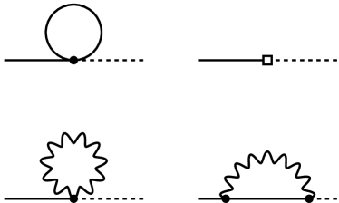
Figure 2: The Feynman diagrams that contribute to the axial current operator at NLO. A filled circle denotes a vertex from the ${\cal L}_{2}$ Lagrangian and an open square denotes a vertex from the ${\cal L}_{4}$ Lagrangian. A straight line is a pseudoscalar meson, a wiggly line is a photon and a dashed line is an axial current.

Diagrams of ${\mathcal{O}}(p^{4},e^{2}p^{2})$ also contribute to Eq. (39) through the wave function renormalization factor $\sqrt{{\mathcal{Z}}}$, since the expression for the decay constant of a meson is

$$\frac{F_{\mathrm{phys}}}{\sqrt{{\mathcal{Z}}}}=F_{0}+F_{4}(M_{\mathrm{phys}}^{2},\chi_{i})+{\mathcal{O}}(p^{6},e^{2}p^{4}).$$ (40)

In Eq. (40), the subscripts of the matrix elements $F$ indicate the chiral order and the lowest order contribution $F_{2}$ has been identified with $F_{0}$. The wave function renormalization is given in terms of the self-energy diagrams by

$${\mathcal{Z}}^{-1} \equiv 1-\left.\frac{\partial\Sigma(p^{2},\chi_{i})}{\partial p^{2}}\right|_{M_{\mathrm{phys}}^{2}}$$ (41)

which becomes, when expanded such that all contributions up to ${\mathcal{O}}(p^{4},e^{2}p^{2})$ are taken into account,

$$\sqrt{{\mathcal{Z}}} = 1\>+\>\frac{\Sigma^{\prime}}{2}\>+\>\cdots$$ (42)

$$\Sigma^{\prime} = \left.\frac{\partial\Sigma_{4}(p^{2},\chi_{i})}{\partial p^{2}}\right|_{M_{\mathrm{phys}}^{2}}\,.$$ (43)

The quantity $\Sigma_{4}$ denotes the one-particle-irreducible diagrams to ${\cal O}(p^{4},e^{2}p^{2})$. Combining these expressions, the decay constant at NLO is then

$$F_{\mathrm{phys}} = F_{0}\>+\>F_{4}(\chi_{i})$$ (44)

$$+ F_{0}\left.\frac{\partial\Sigma_{4}(p^{2},\chi_{i})}{2\,\partial p^{2}}\right|_{M_{0}^{2}}+{\mathcal{O}}(p^{6},e^{2}p^{4})\,.$$

Again it is sufficient to use the lowest order mass $M_{0}^{2}$ in $\Sigma_{4}$ since the diagrams in that term are already of $\mathcal{O}(p^{4},e^{2}p^{2})$. The analytical results for the decay constant are below given in the form

$$F_{\mathrm{phys}}=F_{0}\left[1+\frac{f^{(4)\mathrm{vs}}}{F_{0}^{2}}+\mathcal{O}(p^{6},e^{2}p^{4})\right],$$ (45)

As for the meson masses, the superscripts (v) and (s) indicate the values of $d_{\mathrm{val}}$ and $d_{\mathrm{sea}}$, respectively.

The NLO contribution to the decay constant for a charged pseudoscalar meson with electromagnetic corrections is for $d_{\mathrm{val}}=1$ and $d_{\mathrm{sea}}=3$ found to be

$$f^{(4)13} = +12L_{4}^{r}\bar{\chi}_{1}+4L_{5}^{r}\chi_{1}$$ (46)

$$+6e^{2}F_{0}^{2}\left[K^{Er}_{1}+K^{Er}_{2}\right]\overline{Q}_{2}$$

$$+2e^{2}F_{0}^{2}\left[K^{Er}_{5}+K^{Er}_{6}\right]q_{p}^{2}$$

$$+2e^{2}F_{0}^{2}K^{Er}_{12}q_{12}^{2}$$

$$+e^{2}F_{0}^{2}\left[4K^{Er}_{18}+2K^{Er}_{19}\right]q_{1}q_{2}$$

$$+1/4\bar{A}(\chi_{e,ps})$$

$$+2e^{2}F_{0}^{2}\bar{B}^{\prime}(\chi_{\gamma},\chi_{1},\chi_{1})q_{12}^{2}\chi_{1}$$

$$-e^{2}F_{0}^{2}\bar{B}_{1}(\chi_{\gamma},\chi_{1},\chi_{1})q_{12}^{2}$$

$$-2e^{2}F_{0}^{2}\bar{B}_{1}^{\prime}(\chi_{\gamma},\chi_{1},\chi_{1})q_{12}^{2}\chi_{1}.$$

For $d_{\mathrm{val}}=2$ and $d_{\mathrm{sea}}=3$ the result is

$$f^{(4)23} = =+12L_{4}^{r}\bar{\chi}_{1}+4L_{5}^{r}\chi_{13}$$ (47)

$$+6e^{2}F_{0}^{2}\left[K^{Er}_{1}+K^{Er}_{2}\right]\overline{Q}_{2}$$

$$+2e^{2}F_{0}^{2}\left[K^{Er}_{5}+K^{Er}_{6}\right]q_{p}^{2}$$

$$+2e^{2}F_{0}^{2}K^{Er}_{12}q_{13}^{2}$$

$$+e^{2}F_{0}^{2}\left[4K^{Er}_{18}+2K^{Er}_{19}\right]q_{1}q_{3}$$

$$-1/12\bar{A}(\chi_{m})R^{v}_{mn13}$$

$$+\bar{A}(\chi_{p})\left[1/6R^{p}_{q\pi\eta}-1/12R^{c}_{p}\right]$$

$$+1/4\bar{A}(\chi_{e,ps})$$

$$-1/12\bar{B}(\chi_{p},\chi_{p},0)R^{d}_{p}$$

$$+2e^{2}F_{0}^{2}\bar{B}^{\prime}(\chi_{\gamma},\chi_{13},\chi_{13})q_{13}^{2}\chi_{13}$$

$$-e^{2}F_{0}^{2}\bar{B}_{1}(\chi_{\gamma},\chi_{13},\chi_{13})q_{13}^{2}$$

$$-2e^{2}F_{0}^{2}\bar{B}_{1}^{\prime}(\chi_{\gamma},\chi_{13},\chi_{13})q_{13}^{2}\chi_{13}.$$

The term containing $R^{v}_{mn13}$ is somewhat tricky to take the limit to the simpler mass cases. The form needed for the simpler cases can be found in Ref. BL1 or in website .

V Discussion of the analytical results

Our analytical results are finite. The renormalization obtained from the $n$-flavour divergences using the arguments presented above and in our earlier work, did cancel those from the loop diagrams. In addition, they agree with earlier PQ$\chi$PT results when the electromagnetic parts are removed as well as with the known results for electromagnetic corrections when removing the partial quenching. We have used the definition of the decay constant with the axial current. This definition has an infrared divergence as can be seen also in our result. We have regulated that divergence with a photon mass $\chi_{\gamma}$. This is the definition which was used in Ref. Neufeld as well. How to relate this to measurable quantities can be found in Ref. Cirigliano .

Which combinations of the new LECs can now be determined from lattice calculations? In the masses 5 independent combinations appear:

$$Y_{1} = K^{Er}_{1}+K^{Er}_{2}-K^{Er}_{7}-K^{Er}_{8}\,,$$

$$Y_{2} = K^{Er}_{9}+K^{Er}_{10}\,,$$

$$Y_{3} = -K^{Er}_{5}-K^{Er}_{6}+2K^{Er}_{10}+2K^{Er}_{11}\,,$$

$$Y_{4} = 2K^{Er}_{5}+2K^{Er}_{6}+2K^{Er}_{18}+K^{Er}_{19}\,,$$

$$Y_{5} = K^{Er}_{8}$$ (48)

These can be determined by varying the charges and quark masses separately. It should be noted that the sea quark charges only have a dependence via $Y_{1}\overline{Q}_{2}\chi_{13}$ with undetermined LECs.

The decay constants depend on the combinations

$$Y_{6} = K^{Er}_{1}+K^{Er}_{2}\,,$$

$$Y_{7} = K^{Er}_{5}+K^{Er}_{6}+K^{Er}_{12}\,,$$ (49)

as well as on $Y_{4}$. It should be noted that the sea quark charges only have a dependence via $Y_{6}\overline{Q}_{2}$ with undetermined LECs.

There is in addition dependence on the sea-quark charges in the chiral logarithms, but this dependence is predicted at NLO.

The individual masses and decay constants depend on the sea quark charges. But since the overall dependence on the sea quark charges appearing with unknown LECs is simple we can easily make combinations where this disappears. We use here the notation

$$M^{2}(\chi_{1},\chi_{3},q_{1},q_{3})$$ (50)

to denote the mass of the meson with valence masses $\chi_{1}$ and $\chi_{2}$ and valence charges $q_{1}$ and $q_{3}$. The quantity

$$\Delta M^{2} = M^{2}(\chi_{1},\chi_{3},q_{1},q_{3})-M^{2}(\chi_{1},\chi_{3},q_{3},q_{3})$$ (51)

$$-M^{2}(\chi_{1},\chi_{1},q_{1},q_{3})+M^{2}(\chi_{1},\chi_{1},q_{3},q_{3})$$

is especially useful. Only the electromagnetic corrections survive and the only dependence on the sea-quark charges is in some of the chiral logarithms. Since these contributions are independent of the LECs, they can be subtracted before making fits with lattice simulations, and hence do not present any problem in this respect. The quantity in Eq. (51) is also directly relevant for the violation of Dashen’s theorem Dashen ; BijnensDashen ,

$$\Delta M^{2}_{D}=(m^{2}_{K^{+}}-m^{2}_{K^{0}})-(m^{2}_{\pi^{+}}-m^{2}_{\pi^{0}})\,.$$ (52)

Dashen’s theorem states that the electromagnetic part of $\Delta M^{2}_{D}$ vanishes. $\Delta M^{2}$ becomes the electromagnetic part of $\Delta M^{2}_{D}$ up to some very small electromagnetic corrrections to the $\pi^{0}$ mass in the isospin limit.

Similarly, differences of decay constants of particles containg valence quarks with the same charges have no dependence on the sea quark charges with unknown LECs. In particular this true for the difference of the pion and kaon decay constant. We define

$$F(\chi_{1},\chi_{3},q_{1},q_{3},\{q_{sea}\})$$ (53)

to be the decay constant of a meson with valence masses and charges as for $M^{2}$ above and sea-quark charges $\{q_{sea}\}$. The quantity

$$\Delta F = \bigg{[}F(\chi_{1},\chi_{3},q_{1},q_{3},\{q_{sea}\})-F(\chi_{1},\chi_{3},0,0,\{0\})$$ (54)

$$-F(\chi_{1},\chi_{1},q_{1},q_{3},\{q_{sea}\})+F(\chi_{1},\chi_{1},0,0,\{0\})\bigg{]}$$

$$/F_{0}\,,$$

is an example of this. It gives the relative electromagnetic corrections to the difference of kaon and pion decay constants. In fact, $\Delta F$ is independent of all the $K^{Er}_{i}$.

VI Numerical results

The whole purpose of this work is that our formulas can be used by the lattice QCD community to perform their fits. We therefore only present some representative numerical results. For the $L_{i}^{r}$ we use the values determined in the NNLO order fit of Ref. ABT2 , called fit 10. For the extra electromagnetic parameters we use the estimates of Ref. BP . There are four combinations of the $K^{Er}_{i}$ estimated there. We simply choose a series of $K_{i}^{Er}$ values that reproduces the combinations estimated there and set all others to zero. The nonzero values we have chosen for illustration are

$$K^{Er}_{5} = 2.85\cdot 10^{-3}\,,\quad K^{Er}_{9}=1.3\cdot 10^{-3}\,,$$

$$K^{Er}_{10} = 4.0\cdot 10^{-3}\,,\quad K^{Er}_{11}=-1.25\cdot 10^{-3}\,,$$

$$C = Z_{E}F_{0}^{4}=4.2\cdot 10^{-5}~{}\mbox{GeV}^{5}\,,$$ (55)

at a subtraction scale $\mu=770$ MeV. Earlier estimates of $C$ are in Refs. Bardeen ; EGPR .

The numerics we present here uses $q_{1}=q_{4}=2/3$ and $q_{2}=q_{3}=q_{5}=q_{6}=-1/3$ and a value of $e$ determined from the measured fine structure constant $\alpha$. We also only quote the electromagnetic part by subtracting the same result with $e=0$.

The lowest order correction to the meson masses vanishes for those with zero total charge. For charged mesons it is equal to

$$M^{2}_{LO}=1.00\cdot 10^{-3}~{}\mbox{GeV}^{2}\,.$$ (56)

This should be compared to the physical mass difference

$$m^{2}_{\pi^{+}}-m^{2}_{\pi^{0}}=1.3\cdot 10^{-3}~{}\mbox{GeV}^{2}\,.$$ (57)

There is no electromagnetic correction to the decay constants at lowest order.

Below we use for convenience the terminology $\pi$ for a meson with both valence masses equal to $\chi_{1}$ and $K$ for a meson with valence masses equal to $\chi_{1}$ and $\chi_{3}$ respectively. The charge label is $+$ for valence quark charges $2/3$ and $-1/3$ and $0$ for valence quark charges $-1/3$ and $-1/3$, i.e. electrically neutral.

We first quote the electromagnetic corrections for $\chi_{1}=\chi_{4}=\chi_{5}$ and $\chi_{3}=\chi_{6}$ with $\sqrt{\chi_{1}}=135$ MeV and $\sqrt{\chi_{13}}=495$ MeV.

$$M^{2}_{\pi^{+}NLO} = 0.45\cdot 10^{-3}~{}\mbox{GeV}^{2}\,,$$

$$M^{2}_{K^{+}NLO} = 1.52\cdot 10^{-3}~{}\mbox{GeV}^{2}\,,$$

$$M^{2}_{\pi^{0}NLO} = -2\cdot 10^{-7}~{}\mbox{GeV}^{2}\,,$$

$$M^{2}_{K^{0}NLO} = -3\cdot 10^{-6}~{}\mbox{GeV}^{2}\,.$$ (58)

This leads to a value of

$$\Delta M^{2}=1.07\cdot 10^{-3}~{}\mbox{GeV}^{2}\,.$$ (59)

In agreement with the large violation of Dashen’s theorem seen in Ref. BP since we used their estimate for the constants and similar values for the other inputs. The electromagnetic corrections for the decay constants with a photon mass $\chi_{\gamma}=(10~{}\mbox{MeV})^{2}$ are

$$F_{\pi^{+}NLO}/F_{0} = 0.0039\,.$$

$$F_{K^{+}NLO}/F_{0} = 0.0056\,,$$ (60)

leading to

$$\Delta F=0.0017\,.$$ (61)

The above results are for the unquenched case. To show the effects of partial quenching we plot the quantities $\Delta M^{2}$ and $\Delta F$ with input values as above and $\chi_{4}=\chi_{5}$ and $\chi_{3}=\chi_{6}=0.5~{}\mbox{GeV}^{2}$ as a function of $\chi_{1}$ and $\chi_{4}$ in Figs. 3 and 4.

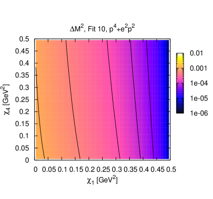
Figure 3: The quantity $\Delta M^{2}$ of Eq. 51, the difference of electromagnetic contributions to meson masses between kaons and pions as a function of the input lowest order masses $\chi_{1}$ and $\chi_{4}$. The scale is logarithmic and contour lines are drawn at $\Delta M^{2}=0.00005,0.0001,0.0002,0.0005,0.001$.

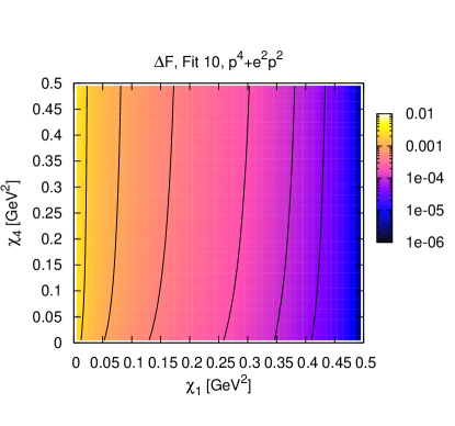
Figure 4: The quantity $\Delta F$ of Eq. 54, the relative difference of electromagnetic contributions to meson decay constants between kaons and pions as a function of the input lowest order masses $\chi_{1}$ and $\chi_{4}$. The scale is logarithmic and contour lines are drawn at $\Delta F=0.00005,0.0001,0.0002,0.0005,0.001,0.002$.

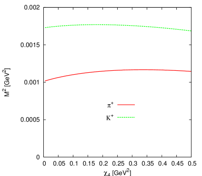
Figure 5: The NLO electromagnetic correction as a function of the sea quark mass $\chi_{4}$ for the case of $\pi^{+}$ and $K^{+}$. See text for the other inputs.

VII Conclusions

In this paper we have shown how to include electromagnetic corrections in partially quenched Chiral Perturbation Theory. We have then used this formalism to compute the electromagnetic corrections to masses and decay constants of the charged or off-diagonal mesons to NLO in PQ$\chi$PT. We also presented some illustrative numerical results.

We have shown that for several phenomenologically interesting quantities the relevant LECs can be computed using quenched photons, i.e. they can be computed with the photons only coupling to the valence quarks.

The dependence on the sea quark mass is rather small in these differences. It cancels to a large extent. In Fig. 5 we show the electromagnetic contribution to the squared mass of the pion and kaon as a function of $\chi_{4}=\chi_{5}$ with $\chi_{1}=0.1~{}\mbox{GeV}^{2}$ and the other inputs as above.

References

• (1) S. Weinberg, Physica A 96, 327 (1979).
• (2) J. Gasser and H. Leutwyler, Ann. Phys.  158, 142 (1984);
• (3) J. Gasser and H. Leutwyler, Nucl. Phys. B 250, 465 (1985).
• (4) A. Morel, J. Phys. (France) 48, 1111 (1987).
• (5) C. W. Bernard and M. F. L. Golterman, Phys. Rev. D 46, 853 (1992) [arXiv:hep-lat/9204007].
• (6) S. R. Sharpe, Phys. Rev. D 46, 3146 (1992) [arXiv:hep-lat/9205020].
• (7) C. W. Bernard and M. F. L. Golterman, Phys. Rev. D 49, 486 (1994) [arXiv:hep-lat/9306005].
• (8) S. R. Sharpe and N. Shoresh, Phys. Rev. D 62, 094503 (2000) [arXiv:hep-lat/0006017].
• (9) S. R. Sharpe and N. Shoresh, Phys. Rev. D 64, 114510 (2001) [arXiv:hep-lat/0108003].
• (10) J. Bijnens, N. Danielsson and T. A. Lähde, Phys. Rev. D 70, 111503 (2004) [arXiv:hep-lat/0406017].
• (11) J. Bijnens and T. A. Lähde, Phys. Rev. D 71, 094502 (2005) [arXiv:hep-lat/0501014].
• (12) J. Bijnens and T. A. Lähde, Phys. Rev. D 72, 074502 (2005) [arXiv:hep-lat/0506004].
• (13) J. Bijnens, N. Danielsson and T. A. Lähde, Phys. Rev. D 73, 074509 (2006) [arXiv:hep-lat/0602003].
• (14) J. Bijnens and N. Danielsson, Phys. Rev. D 74, 054503 (2006) [arXiv:hep-lat/0606017].
• (15) R. F. Dashen, Phys. Rev.  183, 1245 (1969).
• (16) P. Langacker and H. Pagels, Phys. Rev. D 8, 4620 (1973).
• (17) J. F. Donoghue, B. R. Holstein and D. Wyler, Phys. Rev. D 47, 2089 (1993).
• (18) J. Bijnens, Phys. Lett. B 306, 343 (1993) [arXiv:hep-ph/9302217].
• (19) K. Maltman and D. Kotchan, Mod. Phys. Lett. A 5, 2457 (1990).
• (20) R. Urech, Nucl. Phys. B 433, 234 (1995) [arXiv:hep-ph/9405341].
• (21) H. Neufeld and H. Rupertsberger, Z. Phys. C 71, 131 (1996) [arXiv:hep-ph/9506448].
• (22) J. Bijnens and J. Prades, Nucl. Phys. B 490, 239 (1997) [arXiv:hep-ph/9610360].
• (23) B. Moussallam, Nucl. Phys. B 504, 381 (1997) [arXiv:hep-ph/9701400].
• (24) J. F. Donoghue and A. F. Perez, Phys. Rev. D 55, 7075 (1997) [arXiv:hep-ph/9611331].
• (25) B. Moussallam, Eur. Phys. J. C 6, 681 (1999) [arXiv:hep-ph/9804271].
• (26) B. Ananthanarayan and B. Moussallam, JHEP 0406, 047 (2004) [arXiv:hep-ph/0405206].
• (27) A. Pinzke, arXiv:hep-ph/0406107.
• (28) J. Gasser, A. Rusetsky and I. Scimemi, Eur. Phys. J. C 32, 97 (2003) [arXiv:hep-ph/0305260].
• (29) A. Duncan, E. Eichten and H. Thacker, Phys. Rev. Lett.  76, 3894 (1996) [arXiv:hep-lat/9602005].
• (30) A. Duncan, E. Eichten and R. Sedgewick, Phys. Rev. D 71, 094509 (2005) [arXiv:hep-lat/0405014].
• (31) N. Yamada, T. Blum, M. Hayakawa and T. Izubuchi [RBC Collaboration], PoS LAT2005, 092 (2006) [arXiv:hep-lat/0509124].
• (32) Y. Namekawa and Y. Kikukawa, PoS LAT2005, 090 (2006) [arXiv:hep-lat/0509120].
• (33) S. Scherer, in Advances in nuclear physics, edited by J.W. Negele and E. Vogt (Kluwer Academic/Plenum Publishers, New York 2003), vol. 27, pp. 277-538 [hep-ph/0210398]; G. Ecker, hep-ph/0011026; A. Pich, hep-ph/9806303.
• (34) J. Bijnens, G. Colangelo and G. Ecker, JHEP 9902, 020 (1999) [arXiv:hep-ph/9902437].
• (35) J. Bijnens, G. Colangelo and G. Ecker, Ann. Phys.  280, 100 (2000) [arXiv:hep-ph/9907333].
• (36) M. Knecht and R. Urech, Nucl. Phys. B 519, 329 (1998) [arXiv:hep-ph/9709348].
• (37) The analytical formulas may be downloaded via:
http://www.thep.lu.se/$\sim$bijnens/chpt.html.
The programs are available on request from the authors.
• (38) M. Peskin and D. Schroeder, “An Introduction to quantum field theory,” Perseus Books, Reading MA, USA (1995).
• (39) V. Cirigliano, M. Knecht, H. Neufeld, H. Rupertsberger and P. Talavera, Eur. Phys. J. C 23, 121 (2002) [arXiv:hep-ph/0110153].
• (40) G. Amorós, J. Bijnens and P. Talavera, Nucl. Phys. B 602, 87 (2001) [arXiv:hep-ph/0101127].
• (41) G. Ecker, J. Gasser, A. Pich and E. de Rafael, Nucl. Phys. B 321, 311 (1989).
• (42) W. A. Bardeen, J. Bijnens and J. M. Gerard, Phys. Rev. Lett.  62, 1343 (1989).
• (43) J. A. Vermaseren, arXiv:math-ph/0010025.