The spectrum of radial, orbital and gluonic excitations of charmonium

Abstract:

We present results for the charmonium spectrum from $N_{f}=2$ dynamical QCD simulations on $12^{3}\times 80$ anisotropic lattices. Using all-to-all propagators we determine the ground and excited states of S, P and D waves and hybrids. We also evaluate the disconnected (OZI suppressed) contribution to the $\eta_{c}$ and $J/\Psi$.

TRINLAT-06/10

1 Introduction

In recent years there has been a resurgence of interest in charmonium physics, both theoretically and experimentally. The charmonium states below threshold are considered important topics for study by lattice QCD. They provide us with a testing ground for lattice heavy quark methods which are also used to determine elements of the CKM matrix involving $b$ quarks. New experiments at CLEO-c aim to confront lattice QCD calculations with extremely precise experimental data from the charm sector. In addition, the discovery of numerous new, and unexplained, bound states such as the $X(3871)$ and the presence of theoretically allowed exotic states has renewed efforts in charm physics.

Lattice QCD can in principle answer many of the outstanding questions but to do so requires high precision numerical simulations.

In these proceedings we present preliminary results from a relativistic simulation of the charmonium spectrum, using all-to-all propagators on a dynamical anisotropic lattice. An earlier study of the spectrum on a smaller volume was presented in Ref. [1]. The charmonium spectrum at finite temperature was also determined in this way and is presented in Refs [2, 3, 4].

2 The dynamical anisotropic action

The gauge action is a two-plaquette Symanzik-improved action. It is written

$$S_{G}=\frac{\beta}{\xi^{0}_{g}}\left\{\frac{5(1+\omega)}{3u^{4}_{s}}\Omega_{s}-\frac{5\omega}{3u^{8}_{s}}\Omega^{(2t)}_{s}-\frac{1}{12u^{6}_{s}}\Omega^{(R)}_{s}\right\}+\beta\xi^{0}_{g}\left\{\frac{4}{3u^{2}_{s}u^{2}_{t}}\Omega_{t}-\frac{1}{12u^{4}_{s}u^{2}_{t}}\Omega^{(R)}_{t}\right\}$$ (1)

where $\Omega_{s,t}^{R,2t}$ refer to simple and rectangular plaquettes in the spatial and temporal directions and $\xi_{g}^{0}$ is the bare anisotropy. The full details are described in Ref [5].

The anisotropic fermion action [6] is written

$$S_{q}=\bar{\Psi}\left[\gamma_{0}\nabla_{0}+\sum_{i}\mu_{r}\gamma_{i}\nabla_{i}\left(1-\frac{1}{\xi_{q}^{0}a_{s}^{2}}\Delta_{i}\right)-\frac{ra_{t}}{2}\Delta_{i0}+\frac{sa_{s}^{3}}{\sum}_{i}\Delta_{i}^{2}+m_{0}\right]\Psi.$$ (2)

where $a_{s}$ and $a_{t}$ ($a_{s}\gg a_{t}$) are the spatial and temporal lattice spacings respectively and $\xi_{q}^{0}$ is the bare anisotropy.

In an anisotropic simulation the bare anisotropies, which are inputs in the gauge and fermion actions must be tuned so that the measured value of the anisotropy in a simulation takes its “target” value. In the quenched theory the gauge and fermion anisotropies can be separately tuned: however in the dynamical theory these must be simultaneously tuned. The details of this tuning for quenched and dynamical QCD are described in Refs. [6, 7, 8].

3 Simulation details

We performed simulations at $N_{f}=2$ on $N_{s}\times N_{t}=12^{3}\times 80$ lattices with 250 configurations at a sea quark mass close to the strange quark mass. The simulation details are summarized in Table 1.

Configurations	250 ($a_{t}m_{c}=0.117,a_{t}m_{\rm sea}=a_{t}m_{\rm light}=-0.057$)
Dilution	time and space even/odd
Physics	S,P,D waves, S wave radial excitations, and hybrids
Volume	$12^{3}\times 80$
$N_{f}$	2
$a_{s}$	$\sim$ 0.17 fm
$a_{t}^{-1}$	$\sim$ 7GeV
$m_{\pi}/m_{\rho}$	$\sim 0.55$

Table 1: Simulation details for this study of charmonium.

The target (renormalised) anisotropy in this study is 6. We found that, in contrast to the quenched case [6] the anisotropy in the charm sector had to be tuned separately to that in the light quark sector to obtain the same renormalised anisotropy. This mass-dependence of $\xi$ in the dynamical theory may be a discretisation effect and is under investigation. The charm quark mass used in the simulation, $a_{t}m_{c}=0.117$, was tuned to obtain the correct $J/\Psi$ mass. We use all-to-all propagators with dilution, no eigenvectors and two noise vectors, as described in Ref. [9], for better signal to noise ratios. An additional advantage of all-to-all propagators is that constructing an extended basis of operators for better overlap with the states of interest is easier than with point propagators. The list of operators used in this study is given in Table 2.

$0^{-+}$	$\gamma_{5}$,$\gamma_{5}(s_{1}+s_{2}+s_{3})$	$2^{++}$	$\gamma_{k}p_{i}+\gamma_{i}p_{k}$
$1^{--}$	$\vec{\gamma}$,$\gamma_{j}(s_{1}+s_{2}+s_{3})$	$2^{-+}$	$\gamma_{5}(2s_{3}-s_{1}-s_{3})$
$1^{+-}$	$\gamma_{5}\vec{p}$	$2^{--}$	$\gamma_{j}(s_{i}-s_{k})$
$0^{++}$	$\vec{\gamma}\cdot\vec{p}$	$3^{--}$	$\vec{\gamma}\cdot\vec{t}$
$1^{++}$	$\vec{\gamma}\times\vec{p}$	$1^{-+}$	$\vec{\gamma}\times\vec{u}$

Table 2: The basis of operators. The notation used for the gluonic paths, denoted with $s_{i},i=1,2,3$, is defined in Ref. [10].

The spin-averaged (1P-1S) splitting is used to set the lattice spacing, yielding $a_{t}=0.028$fm and $a_{s}=0.17$fm.

Since time dilution introduces a random noise source at each timeslice, effective masses fluctuate more from timeslice to timeslice than is usually seen with point propagators making it difficult to identify a good plateau region. However, these fluctuations do not affect exponential fits and can be reduced further by increasing the dilution level. A more accurate reflection of the quality of the data and stability of the fits can be seen from a sliding window plot. For a fixed value of $t_{\rm max}$ the fitting window, $(t_{\rm min},t_{\rm max})$ is varied by changing $t_{\rm min}$. The sliding window plots show the fitted masses at each interval as a function of $t_{\rm min}$. Sliding window plots for 1S and 2S states of $J/\psi$ are shown in Figure 1.

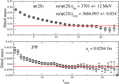
Figure 1: Sliding window plots for the ground and first excited states of the $J/\psi$ at zero momentum. The solid lines show the final best-fitted masses chosen.

The plots show that the 1S fitted mass is stable as $t_{\rm min}$ is varied over twenty timeslices and the 2S mass is stable over seven values of $t_{\rm min}$. For all the fitted masses shown here the quality of the fit is determined and the stable regions also have good $\chi^{2}/N_{\rm d.f.}$. The other charmonium states studied also show extremely stable fitted masses. Based on this analysis the hyperfine splitting is approximately 30 MeV in contrast to the experimental value of 117MeV. The reason for this underestimate is not known yet and will be investigated in future work. In particular, the lattice spacing in this study is quite coarse and the action does not include a $\Sigma\cdot B$ term. In addition it is known from previous work that the hyperfine splitting increases with decreasing lattice spacing and for lighter sea quark masses in dynamical simulations. These improvements will be included in future simulations.

To determine the radially excited states we use a variational basis of operators included extended operators. Our results for the ground state mass using this approach agrees within two percent with the same state determined from exponential fits. Two smearings and two different operators were used to increase the variational basis when determining the $\eta_{c}$ and $J/\Psi$. The first excited state of the $\eta_{c}$ and $J/\Psi$ are $m_{\eta_{c}(2S)}=3645\pm 12$ MeV and $m_{\Psi(2S)}=3701\pm 12$ MeV respectively. This analysis is being extended to the P and D waves. Our preliminary charmonium spectrum, including the P-waves, D-waves and the $1^{-+}$ hybrid is shown in Figure 2.

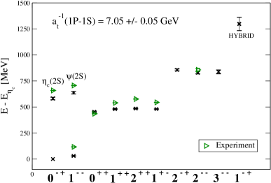
Figure 2: The $c\bar{c}$ spectrum which is normalised to the $\eta_{c}$ mass. The scale has been set from the $(1P-1\bar{S})$ splitting. Experimental values, where known, are denoted with right-facing triangles.

4 Disconnected diagrams

In most lattice calculations of the charmonium spectrum and the hyperfine splitting in particular, the effects of disconnected diagrams in the two point correlator are ignored. It has been estimated that these OZI-suppressed diagrams may in fact contribute $\sim$ 20 MeV to the hyperfine splitting [11, 12], bringing traditionally low lattice determinations into better agreement with experiment. However, the inclusion of such diagrams is not easy, requiring all-to-all propagators which in the past have resulted in noisy data from which it is difficult to extract a convincing signal. It is hoped that the all-to-all propagator algorithm used here may solve this problem using the appropriate dilution to reduce noise. In this first attempt the diagrams were directly calculated using the same dilution already described (time and space). We found that the disconnected diagrams are still noisy and in fits to the full correlator, given by the difference of the connected and disconnected correlators the fit window is reduced to ten data points. Sliding window plots for the full correlators, $C_{\rm full}(t)=C_{\rm connected}(t)-C_{\rm disconnected}(t))$ are shown in figure 3.

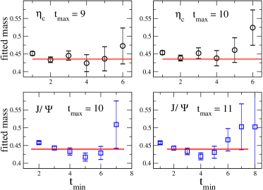
Figure 3: Sliding window plots showing the fitted mass in lattice units for the full correlators, $C_{full}=C_{conn}-C_{dis}$ for the $\eta_{c}$ and $J/\psi$. The plots show the effect of changing $t_{\rm max}$ in the fits. The poor quality of the signal means $t_{\rm max}$ has been moved in from the centre of the lattice approximately timeslice ten. The straight line represents the ground state mass obtained from the connected parts of the correlators.

The plots show no discernible difference after including the disconnected contributions, however we are currently investigating other dilution schemes to optimise the signal.

5 Conclusions

We have presented our preliminary results from a simulation of the charmonium spectrum on $N_{f}=2$ dynamical $12^{3}\times 80$ anisotropic lattices. All-to-all propagators and a variational basis of operators have been used the determine the spectrum of S, P and D waves, their radial excitations as well as the $1^{-+}$ hybrid with good statistical precision. In addition, we have investigated the effects of the disconnected diagrams on the hyperfine splitting. We find a negligible difference. However, these preliminary results need to be investigated further. In particular we are planning to explore dilution strategies and study the volume dependence of the higher excited states.

References

- [1] K. J. Juge, A. O’Cais, M. B. Oktay, M. J. Peardon and S. M. Ryan, PoS LAT2005, 029 (2006), [hep-lat/0510060].
- [2] C. Allton et al., PoS LAT2006, 126 (2006), [hep-lat/0610065].
- [3] G. Aarts et al., hep-lat/0608009.
- [4] R. Morrin et al., PoS LAT2005, 176 (2006), [hep-lat/0509115].
- [5] C. Morningstar and M. J. Peardon, Nucl. Phys. Proc. Suppl. 83, 887 (2000), [hep-lat/9911003].
- [6] TrinLat, J. Foley, A. Ó Cais, M. Peardon and S. M. Ryan, Phys. Rev. D73, 014514 (2006), [hep-lat/0405030].
- [7] R. Morrin, M. Peardon and S. M. Ryan, PoS (LAT2005) 236 [hep-lat/0510016].
- [8] R. Morrin, A. O. Cais, M. Peardon, S. M. Ryan and J.-I. Skullerud, Phys. Rev. D74, 014505 (2006), [hep-lat/0604021].
- [9] J. Foley et al., Comput. Phys. Commun. 172, 145 (2005), [hep-lat/0505023].
- [10] UKQCD, P. Lacock, C. Michael, P. Boyle and P. Rowland, Phys. Rev. D54, 6997 (1996), [hep-lat/9605025].
- [11] UKQCD, C. McNeile and C. Michael, Phys. Rev. D70, 034506 (2004), [hep-lat/0402012].
- [12] QCD-TARO, P. de Forcrand et al., JHEP 08, 004 (2004), [hep-lat/0404016].