Twisted mass QCD for weak matrix elements

Abstract:

I report on the application of tmQCD techniques to the computation of hadronic matrix elements of four-fermion operators. Emphasis is put on the computation of $B_{K}$ in quenched QCD performed by the ALPHA Collaboration. The extension of tmQCD strategies to the study of neutral $B$-meson mixing is briefly discussed. Finally, some remarks are made concerning proposals to apply tmQCD to the computation of $K\to\pi\pi$ amplitudes.

1 Introduction: Flavour Physics vs lattice systematics

During the last five years, a new generation of experimental facilities dominated by B factories have brought Flavour Physics to the era of precision studies. Uncertainties on decay and mixing amplitudes of kaons, $D$- and $B$-mesons have plummeted, setting more stringent constraints than ever on the accuracy required for theoretical estimates aimed at determining Standard Model (SM) parameters or probing new physics. Indeed, although a determination of CKM matrix elements essentially free from hadronic uncertainties starts to be possible [1], knowing all the relevant matrix elements to the required precision is still essential in order to check the consistency of SM predictions and set bounds on effects beyond the SM.

The requirement of few percent accuracy demands, in particular, a fully first-principles approach to the long-distance regime of strong interactions in which all the systematics is consciously brought under control. Mandatory features include:

• Dynamical simulations with at least $2(\mbox{{\em light}})+1$ flavours of sea quarks.

• Good conceptual control over the regularisation.

• Good control of all the symmetries (especially: flavour symmetries).

• Fully non-perturbative renormalisation of all the composite operators involved.

• Elimination of cutoff dependences.

Wilson and chirally symmetric fermions are preferred on conceptual grounds. Wilson fermions have disadvantages from the point of view of flavour symmetries and treatment of ultraviolet cutoff dependencies, but are already able to approach the light quark regime in dynamical simulations [2, 3, 4, 5, 6], although recent progress with dynamical chiral fermions has proved equally impressive (see [7] and references therein). Twisted mass QCD (tmQCD) is a variant of the Wilson regularisation that potentially allows for a better control of chiral symmetry breaking and cutoff effects, which turns particularly advantageous in the computation of weak matrix elements. In this context, it may offer a convenient compromise between an adequate control over chiral symmetry and numerical affordability. Precision quenched computations, that properly deal with all the systematics apart from dynamical quark effects, are an essential step in order to understand these issues and prepare the terrain for dynamical studies. Not least importantly, they offer sound arguments for the choice of regularisation both for sea quarks and for the valence sector of mixed action approaches.

This paper deals mainly with quenched numerical results for weak matrix elements obtained from tmQCD. In Section 2 the ALPHA Collaboration computation of $B_{K}$ in tmQCD [8] is discussed. Section 3 briefly reviews the extension of the strategy to deal with neutral $B$-meson mixing amplitudes, and reports on the project status. Section 4 deals with tmQCD proposals to study $K\to\pi\pi$ amplitudes. Finally, in Section 5 some final remarks are made.

Much of the work presented [8, 9, 10, 11] is part of the ALPHA Collaboration research programme. General reviews of progress in kaon and $B$-physics on the lattice have been provided at this conference by W. Lee and T. Onogi [12, 13].

2 $B_{K}$ in quenched (tm)QCD

2.1 Lattice QCD and indirect CP violation in kaon decays

Indirect CP violation in $K\to\pi\pi$ decays is measured by the parameter $\varepsilon_{K}$, defined in terms of kaon decay amplitudes as

$$\varepsilon_{K}=\frac{T(K_{L}\to(\pi\pi)_{I=0})}{T(K_{S}\to(\pi\pi)_{I=0})}\,,$$ (1)

where $I$ is the total isospin of the two-pion state. Experiment yields [14]

$$\varepsilon_{K}=[2.232(7)\times 10^{-3}]\,\,e^{i\phi_{\varepsilon}}\,,~{}~{}~{}~{}\phi_{\varepsilon}=(43.5\pm 0.7)^{\circ}\,.$$ (2)

At leading order in an Operator Product Expansion (OPE) treatment of electroweak interactions, the Standard Model (SM) prediction for $|\varepsilon_{K}|$ can be written as [15]

$$|\varepsilon_{K}|\simeq C_{\varepsilon}\hat{B}_{K}{\rm Im}\{V_{td}^{*}V_{ts}\}\left\{{\rm Re}\{V_{cd}^{*}V_{cs}\}\left[\eta_{1}S_{0}(x_{c})-\eta_{3}S_{0}(x_{c},x_{t})\right]-{\rm Re}\{V_{td}^{*}V_{ts}\}\eta_{2}S_{0}(x_{t})\right\}\,.$$ (3)

Here $C_{\varepsilon}=G_{\rm F}^{2}F_{K}^{2}M_{K}M_{W}^{2}/(6\sqrt{2}\pi^{2}\Delta M_{K})$, $S_{0}(x_{t})$ and $S_{0}(x_{c},x_{t})$ ($x_{i}=m_{i}^{2}/M_{W}^{2}$) parameterise the Wilson coefficients of the OPE, $\eta_{1,2,3}$ are short-distance QCD corrections to the latter (known to NLO), and

$$\hat{B}_{K}=\frac{\langle\bar{K}^{0}|\hat{O}^{\Delta S=2}|K^{0}\rangle}{\frac{8}{3}F_{K}^{2}M_{K}^{2}}\,,$$ (4)

where $\hat{O}^{\Delta S=2}$ is the effective four-quark interaction operator

$$O^{\Delta S=2}=(\bar{s}\gamma_{\mu}^{\rm L}d)(\bar{s}\gamma_{\mu}^{\rm L}d)\,,$$ (5)

$\gamma_{\mu}^{\rm L}=\gamma_{\mu}(\mathbf{1}-\gamma_{5})$, and the hat denotes renormalisation group invariant (RGI) matrix elements. The dimensionless parameter $\hat{B}_{K}$ thus provides the long-distance, non-perturbative QCD contribution, and largely dominates the uncertainty on the SM value for $|\varepsilon_{K}|$. In the standard Unitarity Triangle (UT) analysis of CP violation in the SM, the value of $|\varepsilon_{K}|$ provides a hyperbola in the $(\bar{\rho},\bar{\eta})$ plane. After the recent generation of experimental results from $B$-factories, this is one of the least precise UT constraints. Improving the accuracy of $\hat{B}_{K}$ is hence essential in order to derive stringent bounds on the amount of non-SM CP violation in kaon decay.

Besides quenching, which is an uncontrolled source of systematic error, the most important source of uncertainty in lattice QCD computations of $B_{K}$ with Wilson fermions arises from operator renormalisation. In standard notation, the operator $O^{\Delta S=2}$ is customarily split into parity-even and parity-odd parts as

$$O^{\Delta S=2}=O_{\rm VV+AA}-O_{\rm VA+AV}\,.$$ (6)

Since parity is a QCD symmetry, the only contribution to the $K^{0}$–$\bar{K}^{0}$ matrix element comes from $O_{\rm VV+AA}$. In regularisations which respect chiral symmetry, the latter operator is multiplicatively renormalisable. If chiral symmetry is not preserved, $O_{\rm VV+AA}$ mixes with four other dimension-6 operators [16, 17, 18, 19, 20] with positive parity:

$$(O_{\rm R})_{\rm VV+AA}(\mu)=Z_{\rm VV+AA}(g_{0},a\mu)\Big{[}O_{\rm VV+AA}(g_{0})+\sum_{i=1}^{4}\Delta_{i}(g_{0})O_{i}(g_{0})\Big{]}$$ (7)

The operators $O_{i}(g_{0})$ belong to different chiral representations than $O_{\rm VV+AA}$. The mixing coefficients $\Delta_{i}(g_{0})$ are finite functions of the bare coupling, while the renormalisation constant $Z_{\rm VV+AA}$ diverges logarithmically in $a\mu$.

Two proposals have attempted to eliminate operator mixing. They are both based on the observation [18, 20] that, even in the absence of chiral symmetry, the operator $O_{\rm VA+AV}$ is protected from finite operator mixing by discrete symmetries, and thus it renormalises multiplicatively, viz.

$$(O_{\rm R})_{\rm VA+AV}(\mu)=Z_{\rm VA+AV}(g_{0},a\mu)O_{\rm VA+AV}(g_{0})\,.$$ (8)

The first proposal [21] consists in obtaining the physical $K^{0}-\bar{K}^{0}$ matrix element of $O_{\rm VV+AA}$ from a correlation function of the renormalised operator $O_{\rm VA+AV}$, related to it through axial Ward identities. The method has been put to test in ref. [22], with the result that the $B_{K}$ estimate turned out to be compatible with the result of computations that involve operator subtractions. Unfortunately, the correlation function of $O_{\rm VA+AV}$ is a four-point function, while the matrix element of $O_{\rm VV+AA}$ can be extracted from a three-point function. Thus, the conclusion of [22] is that this method is successful in eliminating an important source of systematic errors (operator subtraction) at the cost of increased statistical fluctuations.

In the work under consideration here, the second proposal [23], based on twisted mass QCD, is implemented. In tmQCD the breaking pattern of flavour symmetries is controlled by the value of the twist angle; in particular, the latter can be tuned so as to preserve part of the axial subgroup, at the price of breaking vector symmetries, as well as parity. It is thus possible to set up regularisations in which the renormalisation of composite operators is greatly simplified. The relevant case for us is the renormalised $\langle\bar{K}^{0}|O_{\rm VV+AA}|K^{0}\rangle$ matrix element, which via the tmQCD formalism can be extracted from a three-point correlation function of the operator $O_{\rm VA+AV}$. As the tmQCD action differs from the standard Wilson fermion action by a soft term, the renormalisation properties of composite operators in mass independent renormalisation schemes are not modified. In particular, $O_{\rm VA+AV}$ remains multiplicatively renormalisable, with the same renormalisation constant and running as with Wilson fermions. Thus finite subtractions are avoided in the tmQCD determination of $B_{K}$.

An obvious alternative to avoid renormalisation problems consists in using regularisations with exact chiral symmetry. However, the computational costs involved make it difficult to perform continuum limit extrapolations and study finite volume effects. In the case of staggered fermions, apart from the operator mixing (the details of which depend on the specific setup), some additional problems are present — large scaling violations unless high levels of $\mbox{O}(a^{2})$ improvement are implemented, uncertainties related to the choice of interpolating operator, as well as other difficulties related to the breaking of flavour symmetries and the presence of unphysical flavours. Wilson fermions therefore offer, a priori, a good compromise between good control of the field-theoretical aspects of the problem and affordable computational costs.

2.2 tmQCD setup

We will employ two different fermion actions, namely

$$S_{\rm F}^{(\pi/2)} =a^{4}\sum_{x}\,\,[\bar{\psi}(x)(D_{\rm w,sw}+m_{l}+i\gamma_{5}\tau^{3}\mu_{l})\psi(x)\,+\,\bar{s}(x)(D_{\rm w,sw}+m_{s})s(x)]\,,$$ (9)

$$S_{\rm F}^{(\pi/4)} =a^{4}\sum_{x}\,\,[\bar{u}(x)(D_{\rm w,sw}+m_{u})u(x)\,+\,\bar{\psi}(x)(D_{\rm w,sw}+m_{l}+i\gamma_{5}\tau^{3}\mu_{l})\psi(x)]\,.$$ (10)

The labels on the two actions refer to the values that will eventually be set for the twist angle. In Eq. (9) $\psi=(u,d)^{T}$, while in Eq. (10) $\psi=(s,d)^{T}$. In both cases, the matrix $\tau^{3}$ acts on flavour space, and $D_{\rm w,sw}$ is the Wilson-Dirac operator with a Sheikholeslami-Wohlert term; $c_{\rm sw}$ is tuned to its non-perturbative value [25]. In Eq. (10) it has been assumed a priori that the $s$ and $d$ quarks have degenerate physical masses; while this is not necessary as long as this action is used in quenched QCD, all the computations carried out with it are performed in that limit. The action in Eq. (9), on the other hand, is perfectly well suited for an unquenched computation, and it has been used to explore the effect of having non-degenerate $s$ and $d$ quark masses (see below).

The properties of tmQCD have been extensively discussed in several publications (see [23, 26, 27] and references therein). Here we just remind some basic facts. The physical renormalised masses of twisted quarks and the twist angle $\alpha$ are given by

$$M_{\rm R} =\sqrt{m_{\rm R}^{2}+\mu_{\rm R}^{2}}\,,$$ (11)

$$\tan\alpha =\frac{\mu_{\rm R}}{m_{\rm R}}\,,$$ (12)

where $m_{\rm R}$ (resp. $\mu_{\rm R}$) are the renormalised standard (twisted) quark masses. In order to tune the twist angle to some prescribed value up to $\mbox{O}(a^{2})$ corrections, we employ the formulae for the construction of $\mbox{O}(a)$ improved renormalised masses

$$m_{{\rm R},l} =Z_{m}[m_{q,l}(1+b_{m}am_{q,l})+\tilde{b}_{m}a\mu_{l}^{2}]\,,$$ (13)

$$\mu_{{\rm R},l} =Z_{\mu}\mu_{l}(1+b_{\mu}am_{q,l})\,,$$ (14)

where $m_{q,l}={\scriptstyle{{1\over 2}}}(1/\kappa-1/\kappa_{\rm c})$ is the subtracted bare standard quark mass.

In the case of the $\pi/2$ regularisation, in order to have $\alpha=\pi/2$ it is enough to set $m_{{\rm R},l}$ to zero, which is achieved by setting

$$am_{q,l}=-\tilde{b}_{m}(a\mu_{l})^{2}\,.$$ (15)

The $\pi/4$ case is somewhat less trivial. Setting $\alpha=\pi/4$ requires $\mu_{{\rm R},l}=m_{{\rm R},l}$, which via Eqs. (13,14) translates into

$$am_{q,l}=\dfrac{1}{ZZ_{A}}a\mu_{l}\big{\{}1+\big{[}\dfrac{1}{ZZ_{A}}(b_{\mu}-b_{m})-ZZ_{A}\tilde{b}_{m}\big{]}a\mu_{l}\big{\}}$$ (16)

with $Z\equiv Z_{m}/(Z_{\mu}Z_{A})$. For a given choice of $a\mu_{l}$, $\kappa$ is tuned so that $am_{q,l}$ satisfies one of the two above relations, taking the values of $\kappa_{\rm c}$ and all the renormalisation constants and improvement coefficients involved as input. The precision to which the latter are known poses an implicit constraint on the accuracy of the tuning of the twist angle.

Contact with QCD is made via the change of fermion variables

$$\psi\to\psi^{\prime}=R(\alpha)\psi,\qquad\bar{\psi}\to\bar{\psi}^{\prime}=\bar{\psi}R(\alpha)\ ,$$ (17)

where $R(\alpha)=\exp\left\{{\scriptstyle{{i\over 2}}}\gamma_{5}\alpha\tau^{3}\right\}$ and $\psi$ is the twisted quark doublet. This axial rotation induces a mapping between composite operators in tmQCD and QCD, which is realised at the level of renormalised correlation functions (or, alternatively, renormalised matrix elements). The relation we are most interested in is

$$\langle K^{0}|\,\,(O_{R})_{\rm VV+AA}\,\,|\bar{K}^{0}\rangle_{\rm QCD}=-i\langle K^{0}|\,\,(O_{R})_{\rm VA+AV}\,\,|\bar{K}^{0}\rangle_{\rm tmQCD}\,,$$ (18)

which holds in the continuum limit for the two versions of tmQCD under consideration. From this identity, $B_{K}$ can be extracted from a $K^{0}$–$\bar{K}^{0}$ matrix element of the multiplicatively renormalisable operator $O_{\rm VA+AV}$.

It is important to stress that none of the above setups leads to a computation of $B_{K}$ that involves fully twisted quarks only. Hence, the automatic $\mbox{O}(a)$ improvement argument of Frezzotti and Rossi [28] does not apply, and in order to have full $\mbox{O}(a)$ improvement of the matrix element it would be necessary to subtract a number of dimension-seven counterterms from the four-fermion operator. Such a procedure is highly impractical, and has not been pursued. Hence, leading cutoff effects in $B_{K}$ are expected to be linear in $a$.

2.3 Renormalisation

The non-perturbative renormalisation of the operator $O_{\rm VA+AV}$ has been addressed in [9, 10] using standard Schrödinger Functional (SF) techniques (see e.g. [29]). After having defined suitable SF intermediate renormalisation schemes, a recursive step-scaling procedure allows to compute to high accuracy the renormalisation group (RG) running of the operator in quenched QCD in the continuum limit from a low-energy reference scale $(2L_{\rm max})^{-1}$ close to $\Lambda_{\rm QCD}$ to scales of $O(100~{}\rm GeV)$, where reliable contact with perturbation theory can be made. Together with the renormalisation constants at $(2L_{\rm max})^{-1}$, this provides RGI renormalisation factors free from any uncontrolled systematic uncertainty.

In the particular case of $O_{\rm VA+AV}$, nine different SF schemes were defined and found to provide consistent results for RGI renormalisation factors. The continuum limit of the RG running was controlled by performing independent simulations with two different fermion actions (plain and $\mbox{O}(a)$ improved Wilson fermions). The quality of the result is illustrated by Figure 1. This approach is currently being pursued in order to extend the non-perturbative renormalisation of $O_{\rm VA+AV}$ to $N_{f}=2$ QCD [30]. It is also worth mentioning that the scope of [9, 10] goes well beyond the case of the $\Delta S=2$ effective Hamiltonian. For instance, [31] made use of the results in [9] to address the renormalisation of the $\Delta S=1$ effective Hamiltonian with an active charm quark constructed with overlap fermions. To that purpose, the logarithmically divergent renormalisation constants required have been computed through a matching of non-perturbatively renormalised RGI tmQCD matrix elements to bare overlap matrix elements at a reference mass $m_{\rm PS}\simeq m_{K}$. This procedure is similar to the one employed in [32] for the renormalisation of the quark condensate.

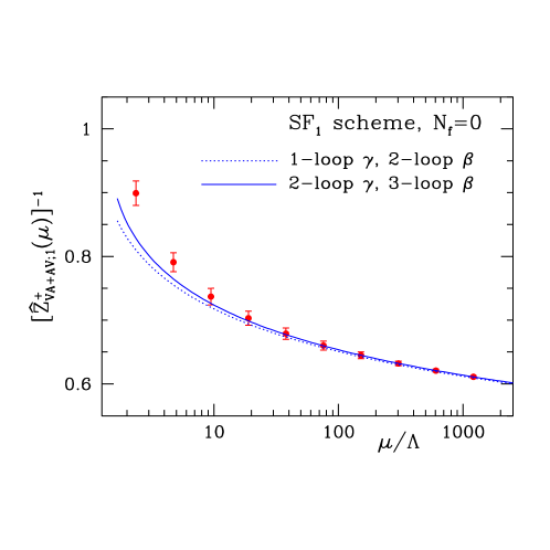
Figure 1: RG running $O_{\rm VA+AV}$ in quenched QCD in the SF scheme. Non-perturbative values (circles) are compared to perturbation theory predictions.

2.4 Simulations for bare matrix elements and systematics

The bare value of $B_{K}$ can be extracted from the ratio of SF correlation functions

$$R(x_{0})=\frac{3}{16}\frac{-if_{\rm VA+AV}(x_{0})}{[Z_{\rm\scriptscriptstyle A}(f_{\rm\scriptscriptstyle A}(x_{0})+c_{\rm\scriptscriptstyle A}a\partial_{0}f_{\rm\scriptscriptstyle P}(x_{0}))-iZ_{\rm\scriptscriptstyle V}f_{\rm\scriptscriptstyle V}(x_{0})][Z_{\rm\scriptscriptstyle A}(f_{\rm\scriptscriptstyle A}^{\prime}(x_{0})+c_{\rm\scriptscriptstyle A}a\partial_{0}f_{\rm\scriptscriptstyle P}^{\prime}(x_{0}))-iZ_{\rm\scriptscriptstyle V}f_{\rm\scriptscriptstyle V}^{\prime}(x_{0})]}\,,$$ (19)

where $f_{\rm VA+AV}$ is the correlation function of $O_{\rm VA+AV}$ with two pseudoscalar SF boundary sources and $f_{\rm\scriptscriptstyle X}$ ($X=A_{0},P,V_{0}$) is a two-point function of the bilinear operator $X$ with a pseudoscalar SF boundary source. Precise definitions can be found in [8]. The combination of currents in the denominator corresponds to the physical, $\mbox{O}(a)$ improved, renormalised axial current via the chiral rotation in Eq. (17).

Quenched simulations have been performed at $\beta=6.0,6.1,6.2,6.3$ for the $\pi/2$ regularisation and $\beta=6.0,6.1,6.2,6.3,6.45$ for $\pi/4$. The physical masses of the $s$ and $d$ quarks have always been kept degenerate, save for a subset of simulations meant to probe $\mbox{SU}(3)$ flavour breaking effects (see below). In the $\pi/2$ case, since the $s$ quark is untwisted, it is impossible to reach pseudoscalar masses in the region of $m_{K}$, due to the presence of exceptional configurations. Therefore, pseudoscalar masses larger than $m_{K}$ are simulated, and the results are hence extrapolated to the physical kaon mass. In the $\pi/4$ case, on the contrary, values at $m_{K}$ can be obtained by interpolation. The necessary renormalisation constants and improvement coefficients, as well as the values of $\kappa_{\rm c}$, have been gathered from the literature. The scale is always fixed via the ratio $r_{0}/a$ as given by [33], with $r_{0}=0.5~{}\rm fm$.

The results have been subjected to a number of checks, meant to assess various systematic uncertainties:

• Finite volume effects. In the $\pi/2$ case, simulations at $\beta=6.0$ have been performed for physical lattice sizes around $L\approx 1.5~{}\rm fm$ and $L\approx 2~{}\rm fm$, at the lowest pseudoscalar meson mass available. Consistent values for all the relevant observables are obtained within errors. Simulations were hence carried out on lattices with $L\sim 1.5~{}\rm fm$. In the $\pi/4$, a similar study was performed at $\beta=6.0,6.2$ and masses around $m_{K}$. In this case the conclusion is that lattice sizes $L\sim 2~{}\rm fm$ are needed to avoid finite volume effects.

• $\mbox{SU}(3)$ breaking effects. Physical $\mbox{SU}(3)$ breaking effects on $B_{K}$ have been studied in the $\pi/2$ case at $\beta=6.0$. To this purpose, simulations were performed for three values of the ratio $\epsilon=(M_{s}-M_{d})/(M_{s}+M_{d})$ (where $M_{f}$ is the physical quark mass), namely $\epsilon=0.00,0.16,0.41$, at fixed $r_{0}m_{\rm PS}=1.78$. No effect was observed on $B_{K}$ within uncertainties, hinting at small $\mbox{SU}(3)$ breaking effects. It has to be stressed, however, that the simulated pseudoscalar mass is relatively high.

• Spurious $\mbox{SU}(3)$ breaking. The $\mbox{O}(a^{2})$ breaking of vector flavour symmetries induced by the presence of the twisted mass term has received considerable attention in the literature (see [26]). In order to check its effect, one can compare the pseudoscalar meson mass obtained for various flavour combinations of twisted and untwisted quarks in the $\pi/2$ case. In the $M_{s}=M_{d}$ limit, the resulting states can be interpreted as belonging to a multiplet of pseudo-Goldstone bosons; hence, deviations from unity in the ratios $(m_{\rm PS}/m^{\prime}_{\rm PS})^{2}$ of squared pseudoscalar masses in different flavour channels quantify the $\mbox{O}(a^{2})$ vector symmetry breaking. The values of these ratios show that the effect is never beyond the few percent level, and converges to zero in the continuum limit. The splitting tends to grow mildly as the quark mass is decreased. These findings contrast, but are by no means incompatible, with the observation of much larger amounts of $\mbox{O}(a^{2})$ flavour breaking at lighter quark masses [34].

After the publication of [8], a more detailed analysis of the accuracy of the tuning of quark masses and twist angles was performed. The quality of the tuning was found to be satisfactory in all cases save for the simulations at $\beta=6.1$, mainly in the $\pi/4$ case. This is signalled e.g. by relatively large differences between the value of the target twist angle, set to $\pi/2$ or $\pi/4$ when tuning the quark masses via Eqs. (13,14), and the value obtained by computing the ratio $\mu_{{\rm R},l}/m_{{\rm R},l}$ with the PCAC quark mass instead of the subtracted quark mass.

The reason for this behaviour has been traced back to the value of $\kappa_{\rm c}$ taken as input from the literature. Indeed, for an accurate determination of $\kappa_{\rm c}$ it is crucial to follow a constant physics condition in the approach to the continuum limit, which fixes the $\mbox{O}(a^{2})$ ambiguities coming from this source. Instead, the value $\kappa_{\rm c}=0.135496$ quoted in [35] comes from an interpolation of data obtained from a constant physics condition at other values of $\beta$. While the effect of relaxing the constant physics requirement was found to be negligible for the data of [35], its impact on the tuning of twist angles is large. The $\beta=6.1$ critical point has been hence determined afresh, obtaining $\kappa_{\rm c}=0.135665(11)$, and $\beta=6.1$ simulations with new mass parameters have been performed. Full details will be provided in a forthcoming publication [36].

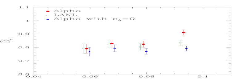
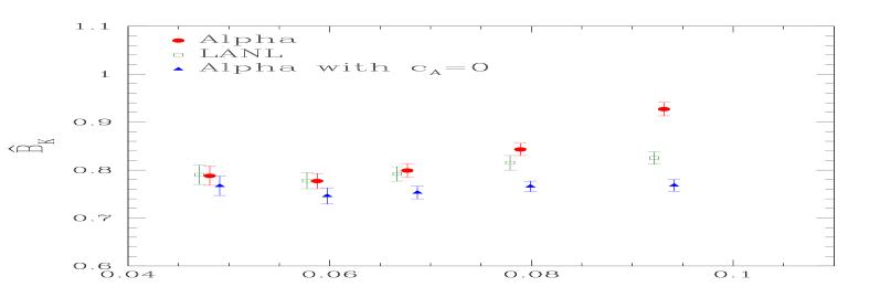
Figure 2: Uncertainties on $\hat{B}_{K}$ related to the $\mbox{O}(a)$ improvement of bilinears. The left panel displays $\pi/2$ data, while the right panel shows $\pi/4$ data.

2.5 Continuum limit

As noted above, taking the continuum limit for $\hat{B}_{K}$ involves a linear extrapolation in $a$. At this stage, having results from two different regularisations, which can be combined in a fit constrained to a common continuum limit, is essential for a proper control of the extrapolation.

It turned out that one of the most relevant sources of cutoff effects is related to the construction of the $\mbox{O}(a)$ improved bilinears in the denominator of Eq. (19). For instance, using either the values for $Z_{\rm\scriptscriptstyle A},Z_{\rm\scriptscriptstyle V},c_{\rm\scriptscriptstyle A}$ determined by the ALPHA Collaboration or those obtained by the LANL group [37] results in sizeable effects on $B_{K}$ at the lowest values of $\beta$ available (see Figure 2). This signals the presence of large $\mbox{O}(a^{2})$ ambiguities in $\hat{B}_{K}$ far from the continuum limit. Combined linear+quadratic extrapolation of the data proved to be unstable. Thus the values of $\beta$ for which the difference between ALPHA and LANL constructions of $\mbox{O}(a)$ improved bilinears results to $\hat{B}_{K}$ discrepancies beyond one sigma were conservatively discarded in the linear fits to the continuum limit. This means that results at $\beta=6.0$ and $\beta=6.1$ had to be left out. The resulting extrapolation is illustrated by the left panel of Figure 3. The final results are:

$$\hat{B}_{K}=0.735(71)\,,$$ (20)

$$\bar{B}_{K}^{{\overline{\rm MS}}}(2~{}\rm GeV)=0.534(52)\,.$$ (21)

When comparing with the result quoted in [8], it has to be taken into account that $\beta=6.1$ data have been revised, for the reasons explained above.

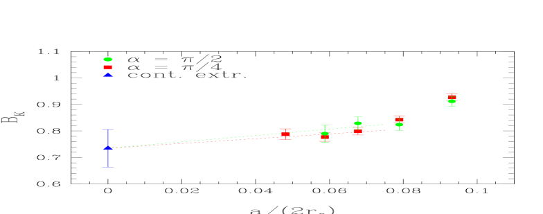
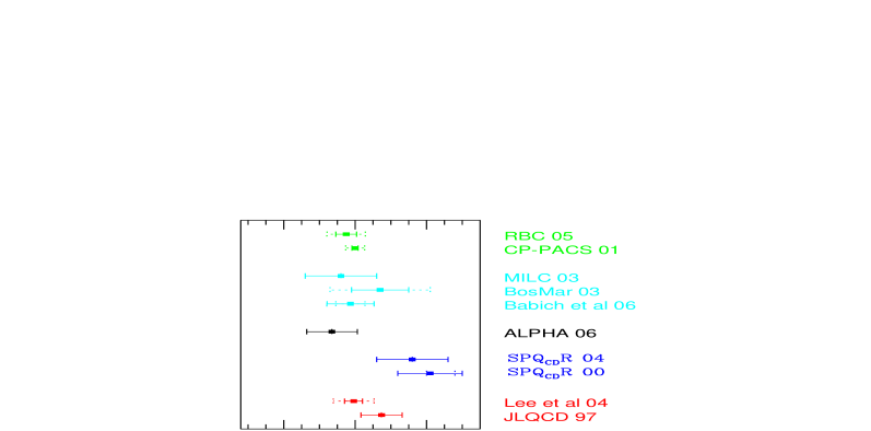
Figure 3: Left: Continuum limit extrapolation of $\hat{B}_{K}$. Right: Comparison with other quenched results.

The value for $\hat{B}_{K}$ in Eq. (20) is shown in the right panel of Figure 3 alongside other representative results in quenched QCD found in the literature. As discussed in Appendix E of [8], the difference with other computations with Wilson fermions is mainly due to the method employed to determine $B_{K}$: instead of using a ratio similar to the one in Eq. (19), the authors of [22] extract $B_{K}$ from a fit of the mass dependence of a different ratio of correlation functions, inspired by Chiral Perturbation Theory. It has to be stressed that the computation of [22] does not have direct access to the physical kaon mass region.

The result of Eq. (20) is the only existing quenched result in the literature which has simultaneously eliminated any systematic uncertainty related to renormalisation (both at a reference scale and from the point of view of RG running), ultraviolet cutoff dependences, and finite volume effects (within the available accuracy). On the other hand, the control of the mass dependence of $\hat{B}_{K}$ with Wilson fermions is still not as accurate as with e.g. Neuberger or domain wall fermions. Overall, it seems fair to claim that Eq. (20) is a benchmark result for $\hat{B}_{K}$ in quenched QCD.

3 A strategy to compute $B_{B}$

Long-distance QCD contributions to indirect CP violation in the $B$-meson sector of the SM are encoded in the bag parameters

$$\hat{B}_{B_{\ell}}=\frac{\langle\bar{B}^{0}|\hat{O}_{\ell}^{\Delta B=2}|B^{0}\rangle}{\frac{8}{3}F_{B_{\ell}}^{2}M_{B_{\ell}}^{2}}\,,$$ (22)

where the relevant effective four-quark interactions have the form

$$O_{\ell}^{\Delta B=2}=(\bar{b}\gamma_{\mu}^{\rm L}\ell)(\bar{b}\gamma_{\mu}^{\rm L}\ell)\,,~{}~{}~{}~{}\ell=d,s\,.$$ (23)

These B-parameters appear, together with the corresponding meson decay constants, e.g. in the expressions for neutral $B$-meson mass differences $\Delta M_{\ell}$ [15]

$$\Delta M_{d} =0.05~{}{\rm ps}^{-1}\,\times\,\bigg{[}\frac{\sqrt{\hat{B}_{B_{d}}}F_{B_{d}}}{230~{}\rm MeV}\bigg{]}\bigg{[}\frac{\bar{m}_{t}(\bar{m}_{t})}{167~{}\rm GeV}\bigg{]}\bigg{[}\frac{|V_{td}|}{0.0078}\bigg{]}\bigg{[}\frac{\eta_{B}}{0.55}\bigg{]}\,,$$ (24)

$$\Delta M_{s} =17.2~{}{\rm ps}^{-1}\,\times\,\bigg{[}\frac{\sqrt{\hat{B}_{B_{s}}}F_{B_{s}}}{260~{}\rm MeV}\bigg{]}\bigg{[}\frac{\bar{m}_{t}(\bar{m}_{t})}{167~{}\rm GeV}\bigg{]}\bigg{[}\frac{|V_{ts}|}{0.040}\bigg{]}\bigg{[}\frac{\eta_{B}}{0.55}\bigg{]}\,,$$ (25)

where $\eta_{B}$ encodes short-distance QCD effects. The experimental values for these quantities are $\Delta M_{d}=0.507\,\pm\,0.005~{}{\rm ps}^{-1}$ [14] and $\Delta M_{s}=17.77\,\pm\,0.10{\rm(stat)}\,\pm\,0.07{\rm(sys)}~{}{\rm ps}^{-1}$ [38]. The recent measurement of $\Delta M_{s}$ by the CDF Collaboration has set very stringent constraints on the required precision of theoretical determinations of $\hat{B}_{B_{s}}F_{B_{s}}^{2}$, which are now at the same level as those on $\hat{B}_{B_{d}}F_{B_{d}}^{2}$. In addition to “standard” systematic uncertainties such as dynamical light quark effects, matrix elements involving heavy quarks are particularly sensitive to improvements coming from a systematic, conceptually controlled treatment of heavy quark effects within lattice QCD.

A strategy for a precise lattice QCD computation of $B_{B_{\ell}}$, which in principle would keep all systematic uncertainties under control, has been put forward in [11]. The $b$ quark is treated at leading order in Heavy Quark Effective Theory (i.e. in the static approximation), although $1/m_{b}$ corrections from the heavy quark expansion can be eventually included following the spirit of [39]. In the static approximation the relevant physical amplitude is a linear combination of matrix elements of two static-light four-fermion operators, viz.

$$O_{1}^{\Delta B=2} =(\bar{h}\gamma_{\mu}^{\rm L}\ell)(\bar{h}\gamma_{\mu}^{\rm L}\ell)\,,~{}~{}~{}~{}\ell=d,s\,,$$ (26)

$$O_{2}^{\Delta B=2} =(\bar{h}(\mathbf{1}-\gamma_{5})\ell)(\bar{h}(\mathbf{1}-\gamma_{5})\ell)\,,~{}~{}~{}~{}\ell=d,s\,.$$ (27)

The renormalisation of generic static-light four-fermion operators with Wilson light fermions has been analysed in detail in [11]. An important conclusion of this study is that, similar to the case of fully relativistic operators, parity-even operators mix between them due to the breaking of chiral symmetry. On the other hand, in the parity-odd sector it is possible to find a complete basis of operators that renormalise multiplicatively. This opens the door to a generalisation to this context of the tmQCD strategy pursued for $B_{K}$. In particular, it is possible to extract $B_{B_{\ell}}$ from matrix elements of the ${\rm VA+AV}$ and ${\rm SP+PS}$ parts of the operators in Eqs. (26,27) if the light quark flavour $\ell$ is twisted at $\alpha=\pi/2$. This avoids any need of dealing with complicated operator renormalisation patterns, and eliminates any constraint on quenched computations due to exceptional configurations. Furthermore, it is possible to extend the automatic $\mbox{O}(a)$ improvement arguments of Frezzotti and Rossi to show that the matrix elements of interest will display scaling violations at $\mbox{O}(a^{2})$ only.

The numerical implementation of non-perturbative renormalisation for static-light four-fermion operators is discussed in detail in [11]. Preliminary results for the RG running of static-light four-fermion operators in quenched QCD are shown in Figure 4. Final results will be the object of a forthcoming publication [40].

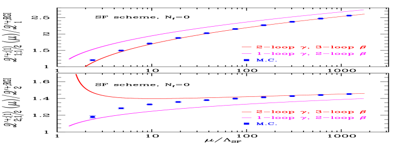
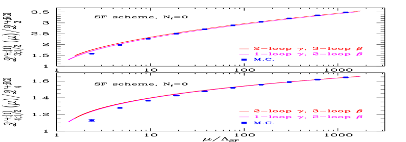
Figure 4: Preliminary results for the non-perturbative RG running (“M.C.” points) of the four independent elements of the multiplicatively renormalisable basis for parity- odd static-light four-fermion operators. See [11] for notational details. The solid curves are perturbative predictions.

4 tmQCD for $K\to\pi\pi$?

The computation of non-leptonic kaon decay amplitudes in QCD poses much harder problems than those related to $\Delta F=2$ processes:

• Finite volume effects strongly affect the two-pion final state, making the direct extraction of the amplitudes from Euclidean correlation functions considerably difficult [41, 42]. It has thus become customary to attempt instead the computation of the relevant couplings in a low- energy effective description of QCD based on Chiral Perturbation Theory, which in principle would allow the computation of the amplitudes at a given order in the chiral expansion [43]. This requires, ideally, access to the chiral regime of QCD.

• The renormalisation of the $\Delta S=1$ effective Hamiltonian arising from the OPE treatment of electroweak interactions requires dealing with a complex operator mixing problem. In particular, if chiral symmetry is not preserved by the lattice regularisation, as with Wilson fermions, mixing with lower dimension operators proceeds via coefficients that diverge with an integer power of the cutoff [44]. On the other hand, if the charm quark is kept as an active degree of freedom the presence of exact lattice chiral symmetry eliminates all power-divergent mixings [45, 46].

The case for employing regularisations that preserve chiral symmetry in the approach to this problem is therefore very strong. Indeed, chiral fermions have been instrumental in a recent computation, in the quenched approximation, of the leading-order low-energy couplings of the $\Delta S=1$ effective weak Hamiltonian in the GIM limit $m_{c}=m_{u}$ [47], the first results of a comprehensive programme aimed at understanding the rôle of the charm quark in the $\Delta I=1/2$ enhancement rule [46, 48]. On the other hand, it is conceivable that the control over chiral symmetry breaking that constitutes one of the main assets of tmQCD can be exploited in order to alleviate the problems related to renormalisation. Two different proposals have been actually put forward to that effect.

In [49], a theory with four quark flavours is considered, without specifying a priori how many of them are dynamical. Once the light doublet is twisted at angle $\pi/2$, it is immediate to show that the power divergences affecting $K\to\pi$ matrix elements are at most linear, and that there are no finite mixings with other dimension six operators. This is a substantial gain with respect to standard Wilson fermions, in which divergences are quadratic and finite mixings are present. If the heavier $s,c$ flavours are fully twisted as well (which is straightforward if they are kept quenched), then it is possible to eliminate power divergences altogether, simply by employing non-perturbatively $\mbox{O}(a)$ improved fermion action and quark bilinears.

In [50], the authors consider a theory in which a valence sector containing an arbitrary number $N_{v}$ of flavours is matched to a theory with $N_{f}$ dynamical quarks. All the flavours are fully twisted. The freedom to fix twist angles arbitrarily for valence quarks, without the need to restrict to non-anomalous chiral rotations, is then used to set up a valence sector that allows to extract $K\to\pi$ matrix elements from correlation functions that do not require any power divergent subtraction. The authors propose a specific valence sector with $N_{v}=10$. In the same paper, a similar technique is proposed to obtain a multiplicatively renormalisable $B_{K}$; in this case, $N_{v}=6$. A strong advantage of this framework is that only fully twisted quarks are used, and hence automatic $\mbox{O}(a)$ improvement arguments apply.

These tmQCD proposals are appealing in that they potentially offer many of the advantages of exactly symmetric regularisations at a considerably lower computational cost. It has to be stressed, however, that the arguments which show that undesired counterterms cancel rely crucially on the assumption that a precise tuning of the twist angle has been performed. In the case of power divergences the issue is particularly sensitive, as systematic uncertainties in the tuning of parameters may result in a lack of cancellation of large contributions to correlation functions. It is important to notice, too, that the absence of exact chiral symmetry poses an intrinsic lower bound to the quark masses that can be simulated safely; in particular, access to the deep chiral regime, as achieved in [47], may be compromised. Finally, the need to separate the $\Delta I=3/2$ and $\Delta I=1/2$ channels requires a good control over the $\mbox{O}(a^{2})$ breaking of isospin symmetry inherent to tmQCD. Given these caveats, the suitability of tmQCD to deal with $K\to\pi\pi$ decays is an open problem that may only be settled by dedicated numerical studies.

5 Conclusions

Twisted mass QCD, together with state-of-the-art techniques for Wilson fermions, allow for benchmark quenched computations of weak matrix elements, as shown by $B_{K}$. The ideas put forward for $\Delta S=2$ matrix elements can be extended to other problems, like $\Delta B=2$ and $K\to\pi\pi$ amplitudes, offering potential for precise computations that do not resort to exact chiral symmetry.

The dominant source of uncertainty left in the quenched approximation (certainly so for $B_{K}$) is related to the lack of full $\mbox{O}(a)$ improvement, which amplifies the error of the continuum limit extrapolation. Thus, if Wilson fermions are to be used in the future in the determination of weak matrix elements, the use of tmQCD variants that embody automatic $\mbox{O}(a)$ improvement [50] may prove essential. Two important aspects of the tmQCD approach are critical in the context of weak matrix elements: the tuning of parameters, in particular of the twist angle, has to be controlled to high precision; and flavour symmetry breaking effects have to be kept at the few percent level. The question whether valence tmQCD quarks offer a convenient alternative to chirally symmetric fermions for some specific applications remains to be addressed by dedicated simulations.

References

- [1] M. Bona et al. [UTfit Collaboration], arXiv:hep-ph/0606167.
- [2] L. Giusti, PoS(LAT2006)009.
- [3] L. Del Debbio, L. Giusti, M. Lüscher, R. Petronzio and N. Tantalo, arXiv:hep-lat/0610059.
- [4] K. Jansen and C. Urbach [ETM Collaboration], PoS(LAT2006)203 [arXiv:hep-lat/0610015].
- [5] M. Gockeler et al., PoS(LAT2006)179 [arXiv:hep-lat/0610066].
- [6] M. Gockeler et al., PoS(LAT2006)160 [arXiv:hep-lat/0610071].
- [7] T. Kaneko et al. [JLQCD Collaboration], PoS(LAT2006)054 [arXiv:hep-lat/0610036].
- [8] P. Dimopoulos et al. [ALPHA Collaboration], Nucl. Phys. B 749 (2006) 69 [arXiv:hep-ph/0601002].
- [9] M. Guagnelli, J. Heitger, C. Pena, S. Sint and A. Vladikas [ALPHA Collaboration], JHEP 0603 (2006) 088 [arXiv:hep-lat/0505002].
- [10] F. Palombi, C. Pena and S. Sint, JHEP 0603 (2006) 089 [arXiv:hep-lat/0505003].
- [11] F. Palombi, M. Papinutto, C. Pena and H. Wittig [ALPHA Collaboration], JHEP 0608 (2006) 017 [arXiv:hep-lat/0604014].
- [12] W. Lee, PoS(LAT2006)015 [arXiv:hep-lat/0610058].
- [13] T. Onogi, these proceedings.
- [14] W.M. Yao et al. [Particle Data Group], J. Phys. G 33 (2006) 1.
- [15] M. Battaglia et al., arXiv:hep-ph/0304132.
- [16] G. Martinelli, Phys. Lett. B141 (1984) 395.
- [17] C. Bernard, T. Draper, and A. Soni, Phys. Rev. D36 (1987) 3224.
- [18] C. Bernard, T. Draper, G. Hockney, and A. Soni, Nucl. Phys. Proc. Suppl. 4 (1998) 483.
- [19] R. Gupta, D. Daniel, G. Kilcup, A. Patel, and S.R. Sharpe, Phys. Rev. D47 (1993) 5113 [arXiv:hep-lat/9210018].
- [20] A. Donini, V. Giménez, G. Martinelli, M. Talevi, and A. Vladikas, Eur. Phys. J. C10 (1999) 121 [arXiv:hep-lat/9902030].
- [21] D. Bećirević et al., Phys. Lett. B487 (2000) 74 [arXiv:hep-lat/0005013].
- [22] D. Bećirević, P. Boucaud, V. Giménez, V. Lubicz, and M. Papinutto, Eur. Phys. J. C37 (2004) 315 [arXiv:hep-lat/0407004].
- [23] R. Frezzotti, P.A. Grassi, S. Sint, and P. Weisz [ALPHA Collaboration], JHEP 08 (2001) 058 [arXiv:hep-lat/0101001].
- [24] R. Babich et al., arXiv:hep-lat/0605016.
- [25] M. Lüscher, S. Sint, R. Sommer, P. Weisz and U. Wolff, Nucl. Phys. B 491 (1997) 323 [arXiv:hep-lat/9609035].
- [26] A. Shindler, PoS(LAT2005) 014 [arXiv:hep-lat/0511002].
- [27] R. Frezzotti, Nucl. Phys. Proc. Suppl. 140 (2005) 134 [arXiv:hep-lat/0409138].
- [28] R. Frezzotti and G.C. Rossi, JHEP 0408 (2004) 007 [arXiv:hep-lat/0306014].
- [29] R. Sommer, Nucl. Phys. Proc. Suppl. 119 (2003) 185 [arXiv:hep-lat/0209162].
- [30] P. Dimopoulos et al. [ALPHA Collaboration], PoS(LAT2006)158 [arXiv:hep-lat/0610077].
- [31] P. Dimopoulos et al., Phys. Lett. B 641 (2006) 118 [arXiv:hep-lat/0607028].
- [32] P. Hernández, K. Jansen, L. Lellouch and H. Wittig, JHEP 0107 (2001) 018 [arXiv:hep-lat/0106011].
- [33] S. Necco and R. Sommer, Nucl. Phys. B 622 (2002) 328 [arXiv:hep-lat/0108008].
- [34] D. Bećirević et al., Phys. Rev. D74 (2006) 034501 [arXiv:hep-lat/0605006].
- [35] J. Rolf and S. Sint [ALPHA Collaboration], JHEP 0212 (2002) 007 [arXiv:hep-ph/0209255].
- [36] P. Dimopoulos et al. [ALPHA Collaboration], in preparation.
- [37] T. Bhattacharya, R. Gupta, W. Lee and S.R. Sharpe, Nucl. Phys. Proc. Suppl. 106 (2002) 789 [arXiv:hep-lat/0111001].
- [38] A. Abulencia et al. [CDF Collaboration], arXiv:hep-ex/0609040.
- [39] J. Heitger and R. Sommer [ALPHA Collaboration], JHEP 0402 (2004) 022 [arXiv:hep-lat/0310035].
- [40] F. Palombi, M. Papinutto, C. Pena and H. Wittig [ALPHA Collaboration], in preparation.
- [41] L. Maiani and M. Testa, Phys. Lett. B245 (1990) 585.
- [42] L. Lellouch and M. Lüscher, Commun. Math. Phys. 219 (2001) 31 [arXiv:hep-lat/0003023].
- [43] C.W. Bernard, T. Draper, A. Soni, H.D. Politzer and M.B. Wise, Phys. Rev. D32 (1985) 2343.
- [44] L. Maiani, G. Martinelli, G.C. Rossi and M. Testa, Nucl. Phys. B289 (1987) 505.
- [45] S. Capitani and L. Giusti, Phys. Rev. D64 (2001) 014506 [arXiv:hep-lat/0011070].
- [46] L. Giusti, P. Hernández, M. Laine, P. Weisz and H. Wittig, JHEP 0411 (2004) 016 [arXiv:hep-lat/0407007].
- [47] L. Giusti et al., arXiv:hep-ph/0607220.
- [48] P. Hernández, these proceedings.
- [49] C. Pena, S. Sint and A. Vladikas, JHEP 0409 (2004) 069 [arXiv:hep-lat/0405028].
- [50] R. Frezzotti and G.C. Rossi, JHEP 0410 (2004) 070 [arXiv:hep-lat/0407002].