First results in QCD with 2+1 light flavors using the fixed-point action

Abstract:

This is a progress report on 2+1 flavor simulation with the FP action on a lattice with spatial size $L=1.2\,\mathrm{fm}$. Since $m_{ud}$ is quite small in our simulation we are in the delta regime for the two light flavors where the low lying excitations are described by a quantum mechanical rotator. From here we extract the low energy constant $F$. We also measure the AWI mass and present results on numerical issues like low-mode averaging and autocorrelation times.

1 Introduction

We performed simulations for $2+1$ light flavors Lattice QCD with the fixed-point Dirac operator. The (parametrized) fixed-point operator we use approximatively satisfies the Ginsparg-Wilson relation [1]:

$$D\gamma_{5}+\gamma_{5}D=D\gamma_{5}2RD\;,$$ (1)

and is limited to a hypercube [2]. (Here $R$ is a non-trivial local matrix.) The quark mass is introduced by

$$D(m)=D+m\left(\frac{1}{2R}-\frac{1}{2}D\right).$$ (2)

The fixed-point action gave very promising results in the quenched approximation, in particular good scaling even at $a=0.15\,\mathrm{fm}$ [3, 4]. We tuned the coupling in our full QCD simulation to be close to $a=0.15\,\mathrm{fm}$ [5], and measurement of the Sommer parameter $r_{0}$ gave a result in agreement with this value. We simulate two lattices, of size $8^{3}\times 24$ and $12^{3}\times 24$ at this coupling. The results presented here refer to the smaller lattice.

2 Autocorrelation times

Figure 1: MC history for the smeared plaquette and the corresponding autocorrelation function.

We estimated the autocorrelation time of plaquettes built from smeared links and that of the pseudoscalar-pseudoscalar correlator. We are using a global update [5], the configurations are separated by $\approx 0.7$ standard Metropolis sweeps.

Fig. 1 shows the MC history for the plaquette for a longer run and the autocorrelation function extracted from it. This gives an autocorrelation time $\tau_{0}\approx 40$.

In Fig. 2 we plot the autocorrelation function for the zero-momentum $\langle P(0)P(t)\rangle$ correlator at different time separations $t$. The autocorrelation time for this quantity is estimated to be somewhat higher.

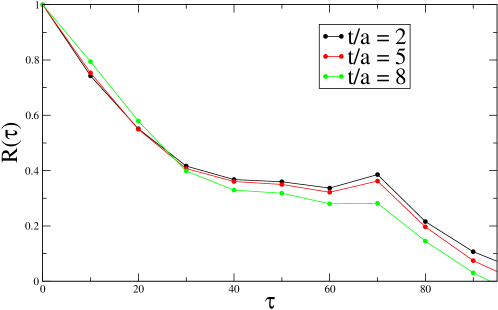
Figure 2: The autocorrelation function for the $\langle P(0)P(t)\rangle$ correlator at different $t$ values.

3 The delta regime

The epsilon regime is defined by:

$$m_{\mathrm{PS}}L,\;m_{\mathrm{PS}}L_{4}\lesssim 1\,,$$ (3)

and the box size should be large enough, $2\pi FL\gg 1$, for the validity of chiral perturbation theory. Here $m_{\mathrm{PS}}$ is the pseudoscalar mass in infinite volume.

In the delta regime [6] one considers a lattice under similar conditions but elongated in the time direction so that the low-lying spectrum in the corresponding spatial volume can be measured. In this regime, for two massless quarks, the low lying spectrum is given by an O(4) rotator having in leading order in $1/L$ a mass gap

$$m_{\mathrm{eff}}=\frac{3}{2F^{2}L^{3}}$$ (4)

Note, however, that for our box size of $L=1.2\,\mathrm{fm}$ one expects non-negligible corrections to this leading order result [7].

4 Low-mode averaging

We used the method of low-mode averaging [8, 9, 10] to decrease the error in the zero-momentum meson correlators

$$C(t;y)=\left.\left\langle\sum_{\vec{x}}\mathrm{tr}\left(\Gamma_{1}\gamma_{5}G(x,y)^{\dagger}\gamma_{5}\Gamma_{2}G(x,y)\right)\right\rangle\right|_{t=x_{4}-y_{4}}\,,$$ (5)

where $\Gamma_{1}$, $\Gamma_{2}$ are arbitrary Clifford algebra matrices. As part of our updating algorithm we calculate the low-lying eigenvalues and their corresponding eigenvectors [5] which allows us to perform such averages. For the $8^{3}\times 24$ lattice we stored $48$ eigenvectors with the smallest eigenvalues. We split up the correlator in Eq. (5) into three parts:

$$C(t;y)=C_{ll}(t)+C_{lh}(t;y_{0})+C_{hh}(t;y)\,,$$ (6)

where $l$ refers to the low-mode part $G_{l}(x,y)$ of the quark propagator (which is given by the calculated eigenvalues and eigenvectors), and $h$ to the rest of the propagator, $G(x,y)=G_{l}(x,y)+G_{h}(x,y)$. We analyze the effects of low-mode averaging for $C_{ll}$ and $C_{lh}$ separately.

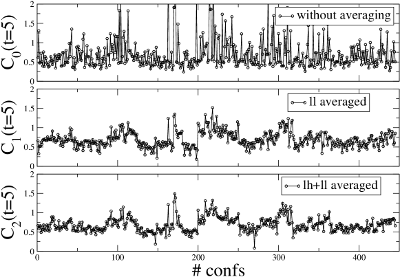
Figure 3: The zero-momentum $\langle P(0)P(t=5)\rangle$ correlator measured at fixed source position ($C_{0}$); by using the eigenvectors to average the source position over the whole lattice in the low-low part ($C_{1}$); by averaging in the source position over a time-slice in the low-high part as well ($C_{2}$).

On Fig.3 we compare the zero momentum correlator $\langle P(0)P(t)\rangle$ at time separation $t=5$ for the different amounts of averaging. $C_{0}$ is the correlator without any averaging over the source position, $C_{1}$ is when the $ll$ part is averaged over the whole volume, $C_{2}$ is when in addition the $lh$ part is also averaged over a time slice. While the $ll$ averaging is very effective, the $lh$ averaging barely shows any suppression of the fluctuations. Since the latter one is also more expensive, one can safely ignore this option and average only in the $ll$ part.

5 Results

5.1 The PCAC mass

Because we are using the parametrized fixed-point action which solves the Ginsparg-Wilson-equation only approximately we get an additive mass renormalization for our PCAC masses. The size of this mass shift is an indicator for the quality of our approximation. From preliminary runs [5] we estimated this additive mass renormalization to be around $0.02$. We ran the present simulations with lattice quark masses $am_{ud}=0.025$, $am_{s}=0.103$. To determine the actual additive mass renormalization we calculated ratios

$$\rho_{ab}(t)=\frac{\langle 0|\partial_{4}^{*}A_{4}^{ab}(t)P_{ba}(0)|0\rangle}{2\langle 0|P_{ab}(t)P_{ba}(0)|0\rangle}\,,\qquad a,b=u,d,s\,.$$ (7)

For both correlator functions we used low-mode averaging and found well-defined plateaus, typically beyond $t\approx 5$. These we denote by $m^{\mathrm{AWI}}_{ab}$. Plotting $m^{\mathrm{AWI}}_{ab}$ against $m_{q}\equiv(m_{a}+m_{b})/2$ and extrapolating in $m_{q}$ to $m^{\mathrm{AWI}}=0$ we obtain the mass shift $m_{0}$. Using naive currents, i.e. the non-conserved axial-vector current in the enumerator and the pseudoscalar density in the denominator of Eq. (7), we also get a multiplicative renormalization factor $Z$:

$$m^{\mathrm{AWI}}_{ab}=Z(m_{q}-m_{0})\,,\qquad m_{q}=\frac{1}{2}(m_{a}+m_{b})\,.$$ (8)

As seen on the left hand side of Fig. 4 the actual values are described very well by this linear dependence. We also plotted on the right hand side of Fig. 4 the $48$ low-lying eigenvalues we stored for several of our configurations with $am_{u}=0.025$ on our $8^{3}\times 24$ lattice. We find that they are lying approximatively on a Ginsparg-Wilson circle shifted by the subtracted mass $am_{\mathrm{sub}}=am_{u}-am_{0}=0.0054(2)$ (corresponding to $7.2(4)\mathrm{MeV}$) away from $\mathrm{Re}\lambda=0$ (red line). The subtracted lattice mass for the strange quark is $am_{s}-am_{0}=0.083$, corresponding to $\approx 110\,\mathrm{MeV}$.

         

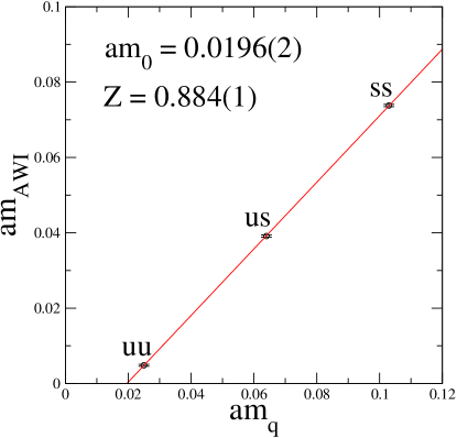
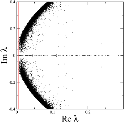
Figure 4: Left: The chiral extrapolation of $m^{\mathrm{AWI}}(m_{q})$ using the combinations ud, us, and ss for the quark flavors. We find an additive mass renormalization of $am_{0}=0.0196(2)$ and a renormalization constant of $Z=0.8837(7)$. Right: The low-lying eigenvalues of the massive Dirac operator for $am_{u}=0.025$. The red line shows the quark mass with this mass shift subtracted, $am_{\mathrm{sub}}=am_{q}-am_{0}$.

5.2 Effective masses

For the point-like pseudoscalar density $P=\overline{\psi}\gamma_{5}\psi$ we calculated the zero-momentum $\langle PP\rangle$ correlator for three different quark flavor combinations (uu,us,ss) and found very stable effective mass plateaus shown in Fig. 5.

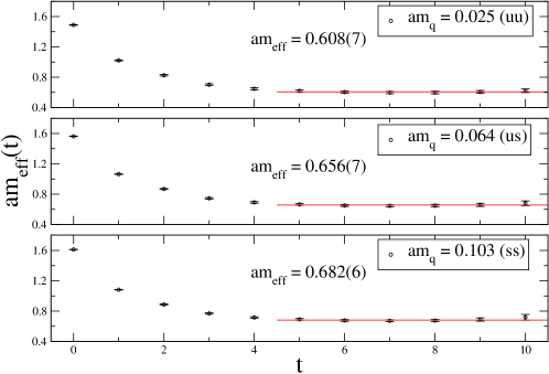
Figure 5: Mass plateau in the $\langle P_{ab}(0)P_{ba}(t)\rangle$ correlator, for $ab=ud,us,ss$.

Linear chiral extrapolation of $m_{\mathrm{eff}}^{2}$ in $m_{q}$ to the chiral limit, shown in Fig. 6, gives:

$$(am_{\mathrm{eff}})^{2}(m_{0})=0.367(6)\;.$$ (9)

Using the finite volume mass gap in lowest order of chiral perturbation theory, Eq. (4), this leads to $F=92.7(4)\,\mathrm{MeV}$ which agrees with the physical value of the pion decay constant, $F_{\pi}=92.4\,\mathrm{MeV}$. However, this agreement is presumably accidental, since the spatial extend of our small lattices is uncomfortably small, and sizeable corrections to the leading order result of Eq. (4) are expected.

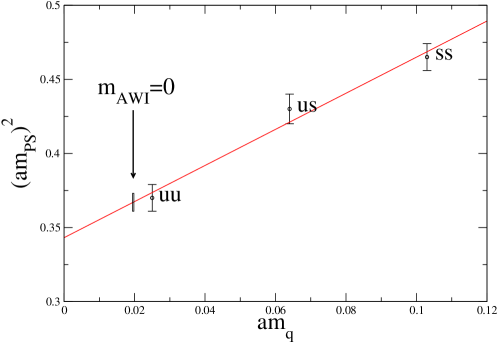
Figure 6: The chiral extrapolations in the pseudoscalar channel. On the right hand side we extrapolate $(am_{\mathrm{eff}})^{2}$ linearly in $am_{q}\to am_{0}$ and on the left hand side we do the same for $am_{\mathrm{eff}}$.

6 Summary and Outlook

We calculated the autocorrelation for the $8^{3}\times 24$ lattice and found autocorrelation times $\tau_{0}\approx 40$ for plaquettes on smeared links and $\tau_{0}\approx 80$ for the $\langle PP\rangle$ correlation functions at fixed time distances.

In the measurement of the meson correlators the low-mode averaging was found to improve the signal significantly. Since the low lying eigenmodes of the Dirac operator were available on each configuration from our updating, this did not require extensive computing resources.

We determined the additive mass renormalization and verified that our light quark masses are near to the chiral limit. We found that the AWI mass depends nearly linearly on the average of the corresponding lattice quark masses. We found that the eigenvalues lie in good approximation on the shifted Ginsparg-Wilson circle.

For the pseudoscalar spectrum we obtained the finite volume mass gap in the chiral limit. Comparing it to the lowest order theoretical prediction we obtained a value for the low energy constant $F$. The surprising agreement with the physical value is presumably an accident since finite volume effects could be quite large at this lattice size.

In the near future we will also have access to larger lattices, on which we plan to analyze conserved currents [4] and all-to-all propagators [11, 12].

7 Acknowledgement

This work was supported in part by Schweizerischer Nationalfonds and by DFG (FG-465). We acknowledge the support and computing resources at CSCS, Manno and LRZ (project h032z).

References

- [1] P. H. Ginsparg and K. G. Wilson, Phys. Rev. D 25, 2649 (1982).
- [2] P. Hasenfratz, Nucl. Phys. Proc. Suppl. 63, 53 (1998) [arXiv:hep-lat/9709110].
- [3] C. Gattringer et al. [BGR Collaboration], Nucl. Phys. B 677, 3 (2004) [arXiv:hep-lat/0307013].
- [4] P. Hasenfratz, S. Hauswirth, T. Jorg, F. Niedermayer and K. Holland, Nucl. Phys. B 643, 280 (2002) [arXiv:hep-lat/0205010].
- [5] A. Hasenfratz, P. Hasenfratz and F. Niedermayer, Phys. Rev. D 72, 114508 (2005) [arXiv:hep-lat/0506024].
- [6] H. Leutwyler, Phys. Lett. B 189, 197 (1987).
- [7] P. Hasenfratz and F. Niedermayer, Z. für Phys. B92 (1993) 91 [arXiv:hep-lat/9212022].
- [8] R. G. Edwards, Nucl. Phys. Proc. Suppl. 106, 38 (2002) [arXiv:hep-lat/0111009].
- [9] T. A. DeGrand and S. Schaefer, Comput. Phys. Commun. 159, 185 (2004) [arXiv:hep-lat/0401011].
- [10] L. Giusti, P. Hernandez, M. Laine, P. Weisz and H. Wittig, JHEP 0404, 013 (2004) [arXiv:hep-lat/0402002].
- [11] J. Foley, K. Jimmy Juge, A. O’Cais, M. Peardon, S. M. Ryan and J. I. Skullerud, Comput. Phys. Commun. 172, 145 (2005) [arXiv:hep-lat/0505023].
- [12] T. Burch and C. Hagen, arXiv:hep-lat/0607029.