Highly Improved Staggered Quarks on the Lattice,
with Applications to Charm Physics.

Abstract

We use perturbative Symanzik improvement to create a new staggered-quark action (HISQ) that has greatly reduced one-loop taste-exchange errors, no tree-level order $a^{2}$ errors, and no tree-level order $(am)^{4}$ errors to leading order in the quark’s velocity $v/c$. We demonstrate with simulations that the resulting action has taste-exchange interactions that are at least 3–4 times smaller than the widely used ASQTAD action. We show how to estimate errors due to taste exchange by comparing ASQTAD and HISQ simulations, and demonstrate with simulations that such errors are no more than 1% when HISQ is used for light quarks at lattice spacings of $1/10$ fm or less. The suppression of $(am)^{4}$ errors also makes HISQ the most accurate discretization currently available for simulating $c$ quarks. We demonstrate this in a new analysis of the $\psi-\eta_{c}$ mass splitting using the HISQ action on lattices where $am_{c}=0.43$ and 0.66, with full-QCD gluon configurations (from MILC). We obtain a result of 111(5) MeV which compares well with experiment. We discuss applications of this formalism to $D$ physics and present our first high-precision results for $D_{s}$ mesons.

I Introduction

The reintroduction of the staggered-quark discretization in recent years has transformed lattice quantum chromodynamics, making accurate calculations of a wide variety of important nonperturbative quantities possible for the first time in the history of the strong interaction ratio-paper ; fk-fpi ; alphas-paper ; fd ; mb-paper . Staggered quarks were introduced thirty years ago, but unusually large discretization errors, proportional to $a^{2}$ where $a$ is the lattice spacing, made them useless for accurate simulations. It was only in the late 1990s that we discovered how to remove the leading errors, and the result was one of the most accurate discretizations in use today. Staggered quarks are faster to simulate than other discretizations, and as a result have allowed us for the first time to incorporate (nearly) realistic light-quark vacuum polarization into our simulations. This makes high-precision simulations, with errors of order a few percent, possible for the first time (see ratio-paper for a more detailed discussion). In this paper we present a new discretization that is substantially more accurate than the improved discretization currently in use. With this new formalism accurate simulations will be possible at even larger lattice spacings, further reducing simulation costs.

The ${\cal O}(a^{2})$ discretization errors in staggered quarks have two sources. One is the usual error associated with discretizing the derivatives in the quark action. The correction for this error is standard and was known in the 1980s naik-paper . The second source was missed for almost a decade. It results from an unusual property of the staggered-quark discretization: the lattice quark field creates four identical flavors or tastes of quark rather than one. (We refer to these unphysical flavors as “tastes” to avoid confusion with the usual quark flavors, which are not identical since quarks of different flavor have different masses.) The missing $a^{2}$ error was associated with taste-exchange interactions, where taste is transferred from one quark line to another in quark-quark scattering. The generic correction for this type of error involves adding four-quark operators to the discretized action.

Taste is unphysical. Instead of one $\pi^{+}$, for example, one has sixteen. Taste is easily removed in simulations provided that different tastes are exactly equivalent, which they are, and provided there are no interactions that mix hadrons of different taste. Taste-exchange interactions, however, cause such mixing, and therefore it is crucial that we understand such interactions and suppress them. Furthermore, past experience suggests that the errors due to residual taste exchange are the largest remaining $a^{2}$ errors in current simulations.

The corrections to the lattice action that suppress taste exchange were missed initially because four-quark operators are not usually needed to correct discretization errors in lowest order perturbation theory (that is, at tree level). They were first discovered empirically from simulations in which the gluon fields in the quark action were replaced by smeared fields, which happen to suppress taste-changing quark-quark scattering amplitudes doug-papers . This discovery led to a proper understanding of the taste-exchange mechanism lepage1-paper ; sinclair-paper , and to the first correct analysis of the $a^{2}$ errors in staggered-quark formalisms lepage1-paper ; lepage2-paper . The resulting “ASQTAD” quark action has provided the basis for almost all simulations to date that include (nearly) realistic light-quark vacuum polarization.

While it is possible to remove all tree-level taste exchange by smearing the gluon fields appropriately, higher-order corrections can only be removed by adding four-quark operators. Recent numerical experiments suggest, however, that even these corrections can be significantly suppressed through additional smearing hyp-paper . These studies, while very important, were limited in two ways. First, they used the mass splittings between the sixteen tastes of pion as a probe for taste exchange; there are many taste-exchange interactions that do not affect this spectrum. Second, smearing the gluon fields introduces other types of ${\cal O}(a^{2})$ error which undo the advantage of an improved discretization (that is, accuracy at large values of $a$).

In this paper we present the first rigorous analysis of one-loop taste exchange. Based upon this analysis we develop a simple smearing scheme that suppresses one-loop corrections by an order of magnitude on average. Our smearing scheme is simpler than that in hyp-paper and, unlike that scheme, it does not introduce new $a^{2}$ errors. The result is a new discretization for highly-improved staggered quarks which we refer to by the acronym HISQ.

An added advantage of a highly improved action is that it can be used to simulate $c$ quarks. Heavy quarks are difficult to simulate using standard discretizations because discretization errors are large unless $am\ll 1$, where $a$ is the lattice spacing and $m$ the quark mass. To simulate $b$ quarks, for example, one would require lattice spacings substantially smaller than $1/20$ fm — much too small to be practical today. Consequently high-quality simulations of $b$ quarks rely upon rigorously defined effective field theories, like nonrelativistic QCD nrqcd , that remove the rest mass from the quark’s energy. While this approach works very well for $b$ quarks, it is less successful for $c$ quarks because the quark’s mass is much smaller, and consequently $c$ quarks are much less nonrelativistic. The smaller quark mass, however, means that $am_{c}\approx 1/2$ for lattice spacings of order $1/10$ fm, which are typical of simulations today. As we demonstrate in this paper, we can obtain few-percent accuracy for charm quarks when $am_{c}\approx 1/2$ provided we use a highly improved relativistic discretization like HISQ.

In Section II we review the (perturbative) origins of taste-exchange interactions in staggered quarks, and their removal at lowest order (tree level) in perturbation theory, using the Symanzik improvement procedure. We also extend the traditional Symanzik analysis to cancel all $(am)^{4}$ errors to leading order in the quark’s velocity, $v/c$ (in units of the speed of light $c$). The additional correction needed is negligible for light quarks, but significantly enhances the precision of $c$-quark simulations.

In Section III, we extend our analysis of taste exchange to one-loop order, and show how to suppress such contributions by approximately an order of magnitude, thereby effectively removing one-loop taste exchange from the theory. The resulting quark action (HISQ) is the first staggered-quark discretization that is both free of lattice artifacts through ${\cal O}(a^{2})$ and effectively free of all taste exchange through one-loop order. We also identify the order $\alpha_{s}(am)^{2}$ corrections to the action that are important for high-precision $c$ physics.

We illustrate the utility of our new formalism, in Section IV, first by examining its effect on taste splittings in the pion spectrum. We also show how to directly measure the size of taste-exchange interactions in simulations, by comparing ASQTAD and HISQ simulations. There has been much discussion recently about the formal significance of taste-exchange interactions creutz-paper-etc . With our procedure it is possible to directly measure the effect of these interactions on physical quantities. We demonstrate the procedure by showing that residual taste-exchange interactions in HISQ contribute less than 1% at current lattice spacings to light-quark quantities such as meson masses and meson decay constants.

We report on a new simulation of $c$ quarks and charmonium using the HISQ formalism in Section V. This is the most severe test of the HISQ formalism since $am_{c}\approx 1/2$ for the lattice spacings we use, but we show that the formalism delivers results that are accurate to a couple of percent, making it the most accurate formalism there is for simulating $c$ quarks. We demonstrate this in a new high-precision determination of the $\psi$–$\eta_{c}$ splitting. This analysis confirms our expectation that the largest $a^{2}$ errors in the ASQTAD action are associated with taste exchange, and we show that these are greatly reduced by using the HISQ action instead.

The moderately heavy smearing used in the HISQ formalism complicates unquenched simulations. In Section VI, we discuss how these complications can be dealt with. Finally, in Section VII, we summarize our results and discuss their relevance to future work. Here we also present our first $D$ physics results from the HISQ action.

Much of our discussion is framed in terms of the “naive” discretization for quarks, which is conceptually equivalent to the staggered-quark discretization (see Appendix B). We usually find naive quarks to be more intuitive in analytic work than staggered quarks, while the latter formalism is definitely the more useful one for numerical work. We outline the formal connection between the naive-quark and staggered-quark formalisms in a series of detailed Appendices. We use these results in our one-loop analysis of taste-exchange interactions, which is described in detail in Appendix F.

We used several sets of gluon configurations in this paper. The parameters for these various sets are summarized in Table 1.

	$a$ (fm)	Gluon Action	$am_{s}$	$am_{u/d}$	$L/a$
UKQCD	$1/10$	Wilson	–	–	16
MILC	$1/8$	Lüscher-Weisz	$0.05$	0.01	20
MILC	$1/11$	Lüscher-Weisz	$0.03$	$0.006$	28

Table 1: Gluon configurations used in this paper with information about the collaboration that produced them, the gluon action used (the unimproved quenched Wilson action or the Symanzik-improved Lüscher-Weisz action for full $n_{f}=3$ QCD), the $s$ and $u=d$ quark masses used in vacuum polarization, and the spatial size of the lattice. The first set of configurations is described in ukqcd-w , while the others are discussed in detail in milc-configs ; ratio-paper .

II Symanzik Improvement for Naive/Staggered Quarks

II.1 Naive Quarks, Doubling, and Taste-Changing Interactions

We begin our review of staggered quarks by examining the formally equivalent “naive” discretization of the quark action (see Appendix B):

$${\cal S}=\sum_{x}\,\overline{\psi}(x)\,(\gamma\cdot\Delta(U)+m_{0})\,\psi(x).$$ (1)

where $\Delta_{\mu}$ is a discrete version of the covariant derivative,

$$\begin{split}\Delta_{\mu}(U)&\,\psi(x)\equiv\\ &\frac{1}{2a}\left(U_{\mu}(x)\,\psi(x+a\hat{\mu})-U^{\dagger}_{\mu}(x-\hat{\mu})\,\psi(x-a\hat{\mu})\right),\end{split}$$ (2)

$U_{\mu}(x)$ is the gluon link-field, $a$ the lattice spacing, and $m_{0}$ is the bare quark mass. The gamma matrices are hermitian,

$$\gamma_{\mu}^{\dagger}=\gamma_{\mu}\quad\quad\gamma_{\mu}^{2}=1\quad\quad\{\gamma_{\mu},\gamma_{\nu}\}=2\,\delta_{\mu\nu},$$ (3)

where indices $\mu$ and $\nu$ run over 0…3. A complete set of sixteen spinor matrices can be labeled by four-component vectors $n_{\mu}$ consisting of 0s and 1s (i.e., $n_{\mu}\in\mathbb{Z}_{2}$):

$$\gamma_{n}\,\equiv\,\prod_{\mu=0}^{3}(\gamma_{\mu})^{n_{\mu}}.$$ (4)

A set of useful gamma-matrix properties is presented in Appendix A.

The naive-quark action has an exact “doubling” symmetry under the transformation:

$$\psi(x)\quad\to\quad\tilde{\psi}(x) \equiv \gamma_{5}\gamma_{\rho}\,(-1)^{x_{\rho}/a}\,\psi(x)$$ (5)

$$= \gamma_{5}\gamma_{\rho}\,\exp(i\,x_{\rho}\pi/a)\,\psi(x).$$

Thus any low energy-momentum mode, $\psi(x)$, of the theory is equivalent to another mode, $\tilde{\psi}(x)$, that has momentum $p_{\rho}\approx\pi/a$, the maximum allowed on the lattice. This new mode is one of the “doublers” of the naive quark action. The doubling transformation can be applied successively in two or more directions; the general transformation is

$$\psi(x)\,\to\,{\cal B}_{\zeta}(x)\,\psi(x)\quad\quad\overline{\psi}(x)\,\to\,\overline{\psi}(x)\,{\cal B}_{\zeta}^{\dagger}(x)$$ (6)

where

$${\cal B}_{\zeta}(x) \equiv \gamma_{\,\overline{\zeta}}\,(-1)^{\zeta\cdot x/a}$$ (7)

$$\propto \prod_{\rho}\,\left(\gamma_{5}\gamma_{\rho}\right)^{\zeta_{\rho}}\,\,\exp(i\,x\cdot\zeta\,\pi/a),$$

and $\zeta$ is a vector with $\zeta_{\mu}\in\mathbb{Z}_{2}$, while $\overline{\zeta}$ is “conjugate” to $\zeta$ (see Appendix A):

$$\overline{\zeta}_{\mu}\equiv\sum_{\nu\neq\mu}\zeta_{\nu}\bmod 2$$ (8)

Consequently there are 15 doublers in all (in four dimensions), which we label with the fifteen different nonzero $\zeta$’s.

As a consequence of the doubling symmetry, the standard low-energy mode and the fifteen doubler modes must be interpreted as sixteen equivalent flavors or “tastes” of quark. (The sixteen tastes are reduced to four by staggering the quark field; see Appendix B.) This unusual implementation of quark tastes has surprising consequences. Most striking is that a low-energy quark that absorbs momentum close to $\zeta\,\pi/a$, for one of the fifteen $\zeta$’s, is not driven far off energy-shell. Rather it is turned into a low-energy quark of another taste. Thus the simplest process by which a quark changes taste is the emission of a single gluon with momentum $q\approx\zeta\,\pi/a$. This gluon is highly virtual, and therefore it must immediately be reabsorbed by another quark, whose taste will also change (see Fig. 1). Taste changes necessarily involve highly virtual gluons, and so are both suppressed (by $a^{2}$) and perturbative for typical lattice spacings. One-gluon exchange, with gluon momentum $q\approx\zeta\,\pi/a$, is the dominant flavor-changing interaction since it is lowest order in $\alpha_{s}(\zeta\pi/a)$ and involves only 4 external quark lines. (Processes with more quark lines are suppressed by additional powers of $(ap)^{3}$ where $p$ is a typical external momentum.) This observation is crucial when trying to improve naive quarks by removing finite-$a$ errors, as we discuss below (see also lepage1-paper ; sinclair-paper ; lepage2-paper ).

Figure 1: The leading tree-level taste-exchange interaction, which involves the exchange of a gluon with momentum $\zeta\pi/a$ where each $\zeta_{\mu}$ is 0 or 1 but $\zeta^{2}\neq 0$.

Sixteen tastes of quark from a single quark field is fifteen too many. In the absence of taste exchange, factors of $1/16$ are easily inserted into simulations to remove the extra copies. In particular, quark vacuum polarization is corrected by replacing the quark determinant in the path integral by its $1/16$ root,

$$\det(\gamma\cdot\Delta+m_{0})\to\det(\gamma\cdot\Delta+m_{0})^{1/16},$$ (9)

or, equivalently, by multiplying the contribution from each quark loop by $1/16$. Recent empirical studies of the spectrum of $\gamma\cdot\Delta$, and improved versions of it, show how eigenvalues cluster into increasingly degenerate multiplets of sixteen as the lattice spacing vanishes, which is necessary if this procedure is to be useful for quark vacuum polarization Dslash-spectrum . The treatment of valence quarks is illustrated in Appendix G.

It is easy to see how the $1/16$ root corrects for taste in particular situations. For example, consider the vacuum polarization of a single pion in a theory of only one massless quark flavor. Ignoring taste exchange, the dominant infrared contributions come from the quark diagrams shown in Fig. 2 (gluons, to all orders, are implicit in these diagrams). The first diagram, with its double quark loop, has contributions from $16^{2}$ identical massless pions, corresponding to configurations where the quark and antiquark each carries a momentum close to an integer multiple of $\pi/a$ (and is therefore close to being on shell). This diagram is multiplied by $1/16^{2}$ since there are two quark loops, thereby giving the contribution of a single massless pion. The second diagram involves quark annihilation into gluons, and has contributions from $16$ identical massless pions, corresponding to configurations where the quark and antiquark each carries a momentum close to the same $\zeta\pi/a$ (so they can annihilate into low-momentum gluons). This diagram is multiplied by $1/16$ since there is only one quark loop, thereby giving the contribution again of a single massless pion but now with an insertion from the gluon decay. Inserting additional annihilation kernels results in a geometric series of insertions in the propagator of a single massless pion that shifts the pion’s mass away from zero, as expected in a $U(1)$ flavor theory.

Figure 2: Infrared contributions from (naive lattice) quark vacuum polarization corresponding to a pion vacuum polarization loop in a simulation of one flavor. The sums are over all infrared sectors, where quarks have momenta near $p_{\mu}=\zeta_{\mu}\pi/a$ for one of the sixteen $\zeta$s consisting of just 0s and 1s. The factors of $1/16$ are from the $1/16$ rule (Eq. (9)) and cancel the sums. Gluons, to all orders, are implicit in these diagrams.

Such patterns are disturbed by taste-exchange interactions like that in Fig. 1. For example, these interactions cause mixing between the different tastes of pion in Fig. 2. This mixing lifts the degeneracy in the pion masses so that different tastes of pion are only approximately equivalent. Consequently the “$1/16$-root rule” gives results that correspond only approximately to a single pion. Taste-changing interactions are suppressed by $a^{2}$, however, and detailed analyses, using chiral perturbation theory, demonstrate that the impact on physical quantities is therefore also suppressed by $a^{2}$ aubin . Consequently, while taste exchange can lead to such anomalies as unitarity violations, these are suppressed in the continuum limit. They are further, and more efficiently, suppressed through Symanzik improvement of the action, as we now discuss.

II.2 Tree-Level Symanzik Improvement

The discretization errors in the naive-quark action come from two sources. The more conventional of these corrects the finite-difference approximation to the derivatives in the action: one replaces naik-paper

$$\Delta_{\mu}\to\Delta_{\mu}-\frac{a^{2}}{6}\Delta_{\mu}^{3}$$ (10)

in the naive-quark action (Eq. (1)). The $a^{2}$ correction is often referred to as the “Naik term.”

Less conventional is a correction to remove leading order taste-exchange interactions lepage1-paper ; sinclair-paper ; lepage2-paper . As discussed in the previous section, these interactions result from the exchange of single gluons carrying momenta close to $\zeta\pi/a$ for one of the fifteen non-zero $\zeta$s ($\zeta_{\mu}\in\mathbb{Z}_{2}$). Since these gluons are highly virtual, such interactions are effectively the same as four-quark contact interactions and could be canceled by adding four-quark operators to the quark action. These operators affect physical results in ${\cal O}(a^{2})$ since they have dimension six. A simpler alternative to four-quark operators is to modify the gluon-quark vertex, $\overline{\psi}\gamma_{\mu}U_{\mu}\psi+\cdots$, in the original action by introducing a form factor $f_{\mu}(q)$ that vanishes for (taste-changing) gluons with momenta $q=\zeta\pi/a$ for each of the fifteen nonzero $\zeta$s. In fact the form factor for direction $\mu$ need not vanish when $\zeta_{\mu}=1$ since the original interaction already vanishes in that case. Consequently we want a form factor where

$$f_{\mu}(q)\to\begin{cases}1&\text{for $q\to 0$}\\ 0&\text{for $q\to\zeta\pi/a$ where $\zeta^{2}\neq 0$, $\zeta_{\mu}=0$}.\end{cases}$$ (11)

We can introduce such a form factor by replacing the link operator $U_{\mu}(x)$ in the action with ${\cal F}_{\mu}U_{\mu}(x)$ where smearing operator ${\cal F}_{\mu}$ is defined by

$${\cal F}_{\mu}\equiv\prod_{\rho\neq\mu}\left.\left(1+\frac{a^{2}\delta^{(2)}_{\rho}}{4}\right)\right|_{\text{symm.}}$$ (12)

and $\delta^{(2)}_{\rho}$ approximates a covariant second derivative when acting on link fields:

$$\delta^{(2)}_{\rho}\,U_{\mu}(x) \equiv\frac{1}{a^{2}}\left(U_{\rho}(x)\,U_{\mu}(x+a\hat{\rho})\,U_{\rho}^{\dagger}(x+a\hat{\mu})\right.$$

$$-2U_{\mu}(x)$$

$$+\left.U_{\rho}^{\dagger}(x-a\hat{\rho})\,U_{\mu}(x-a\hat{\rho})\,U_{\rho}(x-a\hat{\rho}+a\hat{\mu})\right).$$ (13)

This works because $\delta^{(2)}_{\rho}\approx-4/a^{2}$ (and ${\cal F}_{\mu}$ vanishes) when acting on a link field that carries momentum $q_{\rho}\approx\pi/a$. This kind of link smearing is referred to as “Fat7” smearing in doug-papers .

Smearing the links with ${\cal F}_{\mu}$ removes the leading ${\cal O}(a^{2})$ taste-exchange interactions, but introduces new ${\cal O}(a^{2})$ errors. These can be removed by replacing ${\cal F}_{\mu}$ with lepage2-paper

$${\cal F}^{\mathrm{ASQTAD}}_{\mu}\equiv{\cal F}_{\mu}-\sum_{\rho\neq\mu}\frac{a^{2}(\delta_{\rho})^{2}}{4}$$ (14)

where $\delta_{\rho}$ approximates a covariant first derivative:

$$\delta_{\rho}\,U_{\mu}(x) \equiv\frac{1}{a}\left(U_{\rho}(x)\,U_{\mu}(x+a\hat{\rho})\,U_{\rho}^{\dagger}(x+a\hat{\mu})\right.$$

$$-\left.U_{\rho}^{\dagger}(x-a\hat{\rho})\,U_{\mu}(x-a\hat{\rho})\,U_{\rho}(x-a\hat{\rho}+a\hat{\mu})\right).$$ (15)

The new term has no effect on taste exchange but (obviously) cancels the ${\cal O}(a^{2})$ part of ${\cal F}_{\mu}$. Correcting the derivative, as in Eq. (10), and replacing links by $a^{2}$-accurate smeared links removes all tree-level ${\cal O}(a^{2})$ errors in the naive-quark action. The result is the widely used “ASQTAD” action lepage2-paper ,

$$\sum_{x}\,\overline{\psi}(x)\,\left(\sum_{\mu}\gamma_{\mu}\left(\Delta_{\mu}(V)-\frac{a^{2}}{6}\Delta_{\mu}^{3}(U)\right)+m_{0}\right)\,\psi(x),$$ (16)

where, in the first difference operator,

$$V_{\mu}(x)\equiv{\cal F}^{\mathrm{ASQTAD}}_{\mu}\,U_{\mu}(x).$$ (17)

In practice, operator $V_{\mu}$ is usually tadpole improved tadpole ; in fact, however, tadpole improvement is not needed when links are smeared and reunitarized tsukuba ; schladming .

II.3 $c$ Quarks

The tree-level discretization errors in the ASQTAD action are ${\cal O}((ap_{\mu})^{4})$, which are negligible ($<1$%) for light quarks. When applied to $c$ quarks, however, these errors will be larger. The most important errors in this case are associated with the quark’s energy, rather than its 3-momentum, since $c$ quarks are typically nonrelativistic in $\psi$s, $D$s and other systems of current interest. Consequently $E\approx m\gg{\bf p}$ and the largest errors are ${\cal O}((am)^{4})$ or 6% at current lattice spacings ($am_{c}\approx 0.5$). Such errors show up, for example, in the tree-level dispersion relation of the quark where:

$$c^{2}(0) \equiv \lim_{{\bf p}\to 0}\frac{E^{2}({\bf p})-m^{2}}{{\bf p}^{2}}$$ (18)

$$= 1+\frac{9}{20}\,(am)^{4}+\frac{1}{7}\,(am)^{6}+\cdots.$$

This dominant (tree-level) error can be removed by retuning the coefficient of the $a^{2}\gamma_{\mu}\Delta_{\mu}^{3}$ (Naik) term in the action:

$$\sum_{x}\,\overline{\psi}(x)\left(\sum_{\mu}\gamma_{\mu}\left(\Delta_{\mu}-\frac{a^{2}}{6}(1+\epsilon)\Delta_{\mu}^{3}\right)+m_{0}\right)\psi(x),$$ (19)

where parameter $\epsilon$ has expansion

$$\begin{split}\epsilon=&-\frac{27}{40}\,(am)^{2}+\frac{327}{1120}\,(am)^{4}-\frac{5843}{53760}\,(am)^{6}\\ &+\frac{153607}{3942400}\,(am)^{8}-\cdots.\end{split}$$ (20)

With this choice, $c^{2}=1+{\cal O}((am)^{12})$. Only the first term in $\epsilon$’s expansion is essential for removing $(am)^{4}$ errors; the remaining terms remove errors to higher orders in $am$ but leading order in $v/c$, the quark’s typical velocity. In practice, terms beyond the first one or two are negligible though trivial to include.

Note that the bare mass $m_{0}$ in the quark action is related to the tree-level quark mass by

$$m_{0}=m\left(1+\frac{3}{80}\,(am)^{4}-\frac{23}{2240}\,(am)^{6}+\cdots\right)$$ (21)

for this choice of $\epsilon$. This formula is useful for extracting the corrected bare quark mass, $m$, from a tuned value of $m_{0}$.

To examine the tree-level errors in this modified ASQTAD action, it is useful to make a nonrelativistic expansion since, as we indicated, heavy quarks are generally nonrelativistic in the systems of interest. This expansion is easy because the action is identical in form to the continuum Dirac equation, and consequently has the same nonrelativistic expansion but with

$$D_{\mu}\to\Delta_{\mu}-\frac{a^{2}}{6}\,(1+\epsilon)\Delta_{\mu}^{3}.$$ (22)

At tree level,

$$\Delta_{\mu}\to\sinh(aD_{t}-am)/a,$$ (23)

when we replace

$$\psi\to\exp(-mt)\,\psi,$$ (24)

where $m$ is the quark mass. This redefinition removes the rest mass from all energies. Expanding in powers of $1/m$, we then obtain the tree-level nonrelativistic expansion of the modified ASQTAD action:

$$\begin{split}&\sum\psi^{\dagger}_{\mathrm{NR}}\left(D_{t}-\frac{\mathbf{D}^{2}}{2m}-c_{K}\,\frac{\mathbf{D}^{4}}{8m^{3}}-\frac{g\sigma\cdot\mathbf{B}}{2m}\right.\\ &\left.+c_{E}\,\frac{ig[\mathbf{D}\cdot,\mathbf{E}]}{8m^{2}}-c_{E}\,\frac{g\sigma\cdot(\mathbf{D}\times\mathbf{E}-\mathbf{E}\times\mathbf{D})}{8m^{2}}+\cdots\right)\psi_{\mathrm{NR}}\end{split}$$ (25)

where

$$c_{K} =1-\frac{9}{10}\,(am)^{4}+\frac{29}{280}\,(am)^{6}-\cdots$$ (26)

$$c_{E} =1-\frac{3}{80}\,(am)^{4}+\frac{23}{2240}\,(am)^{6}-\cdots.$$ (27)

The coefficients of all terms through order $1/m$ have no $am$ errors at tree level. In particular the $\sigma\cdot\mathbf{B}$ term is correct at tree level once $m$ is tuned (nonperturbatively). The coefficients of the remaining terms shown are off by less than 6% and 1% for charm quarks on current lattices ($am\approx 1/2$), which should lead to errors of order $(am)^{4}(v/c)^{2}\approx 2$% or less in charmonium analyses and less than 0.5% for $D$ physics. (Errors should actually be considerably smaller than this because of dimensionless factors like the $1/8$ in the $\mathbf{D}^{4}$ term.) Other tree-level errors, which are order $(a{\bf p})^{4}$ and $\epsilon(a{\bf p})^{2}/6$, should also be less than 1% for $a\approx 0.1$ fm.

III Symanzik Improvement at One-Loop Order

One-loop errors, which are ${\cal O}(\alpha_{s}(ap)^{2})$, should be no more than a percent or so for light quarks and current lattice spacings. Taste-changing errors, however, have generally been much larger than expected. These errors also bear directly on the validity of the $1/16$-root trick for accounting for taste in the vacuum polarization. For this reason it is worth trying to further suppress taste-exchange errors beyond what has been accomplished at tree level. We show how to do this in this section.

The only other one-loop effects that are important at the level of a few percent are $\alpha_{s}(am)^{2}$ for heavy quarks, and, in particular, the charm quark. We show how to correct for these errors in the Section III.2.

III.1 Light Quarks

One-loop taste exchange comes only from the diagrams shown in Fig. 3; other one-loop diagrams vanish because of the tree-level improvements. Again the gluons in these diagrams transfer momenta of order $\zeta\pi/a$, and so are highly virtual. Consequently, the correction terms in the corrected action that cancel these will involve current-current interactions that conserve overall taste (because of momentum conservation). There are 28 such terms in the massless limit for the staggered-quark action (see Appendix F):

$$\begin{array}[]{r@{\,}l@{}c@{\,}l}2\,\Delta\mathcal{L}_{\text{contact}}=&d_{5}^{(5\mu)}\left|\mathcal{J}_{5}^{(5\mu)}\right|^{2}&+&d_{5\mu\nu}^{(5\nu)}\left|\mathcal{J}_{5\mu\nu}^{(5\nu)}\right|^{2}\\ +&d_{\nu}^{(\mu\nu)}\left|\mathcal{J}_{\nu}^{(\mu\nu)}\right|^{2}&+&d_{5\nu}^{(5\mu\nu)}\left|\mathcal{J}_{5\nu}^{(5\mu\nu)}\right|^{2}\\ +&d_{\mu\nu}^{(\nu)}\left|\mathcal{J}_{\mu\nu}^{(\nu)}\right|^{2}&+&d_{1}^{(\mu)}\left|\mathcal{J}_{1}^{(\mu)}\right|^{2}\\ +&d_{5\mu}^{(5)}\left|\mathcal{J}_{5\mu}^{(5)}\right|^{2}&+&\\ +&d_{1}^{(5\mu)}\left|\mathcal{J}_{1}^{(5\mu)}\right|^{2}&+&d_{\mu\nu}^{(5\nu)}\left|\mathcal{J}_{\mu\nu}^{(5\nu)}\right|^{2}\\ +&d_{\nu}^{(5\mu\nu)}\left|\mathcal{J}_{\nu}^{(5\mu\nu)}\right|^{2}&+&d_{5\nu}^{(\mu\nu)}\left|\mathcal{J}_{5\nu}^{(\mu\nu)}\right|^{2}\\ +&d_{5\mu\nu}^{(\nu)}\left|\mathcal{J}_{5\mu\nu}^{(\nu)}\right|^{2}&+&d_{5}^{(\mu)}\left|\mathcal{J}_{5}^{(\mu)}\right|^{2}\\ &&+&d_{\mu}^{(5)}\left|\mathcal{J}_{\mu}^{(5)}\right|^{2}\\ \end{array}$$ (36)

$$\phantom{\Delta\mathcal{L}\,\,}+\left(\text{color octet $\mathcal{J}$s with $d_{n}^{(t)}\to\tilde{d}^{(t)}_{n}$}\right),$$

where sums over indices are implicit and $\nu\neq\mu$. The currents $\mathcal{J}^{(s)}_{n}$ in the first 14 operators are color-singlets with taste $s$ and spinor structure $n$, while the last 14 operators are the same but with color octet currents. The precise definitions of these currents are given in Appendix E.

Figure 3: The only one-loop diagrams that result in $q\overline{q}\to q\overline{q}$ taste exchange for ASQTAD quarks. Diagrams with additional external quark lines are suppressed by additional powers of $a^{2}$.

	Unimproved Gluons			Improved Gluons
	ASQTAD	HISQ	HYP	ASQTAD
Octet:
$\tilde{d}_{5}^{(5\mu)}$	1.41	0.19	0.02	0.77
$\tilde{d}_{5\mu\nu}^{(5\nu)}$	0.46	0.00	0.08	0.25
$\tilde{d}_{1}^{(5\mu)}$	0.23	0.01	0.00	0.16
$\tilde{d}_{\mu\nu}^{(5\nu)}$	0.38	0.02	0.01	0.27
$\tilde{d}_{\nu}^{(\mu\nu)}$	0.34	0.08	0.04	0.19
$\tilde{d}_{5\nu}^{(5\mu\nu)}$	0.35	0.03	0.02	0.19
$\tilde{d}_{\nu}^{(5\mu\nu)}$	0.08	0.00	0.01	0.05
$\tilde{d}_{5\nu}^{(\mu\nu)}$	0.20	0.00	0.01	0.13
$\tilde{d}_{\mu\nu}^{(\nu)}$	0.20	0.01	0.02	0.11
$\tilde{d}_{1}^{(\mu)}$	0.31	0.01	0.01	0.17
$\tilde{d}_{5\mu\nu}^{(\nu)}$	0.06	0.00	0.00	0.04
$\tilde{d}_{5}^{(\mu)}$	0.07	0.00	0.01	0.04
$\tilde{d}_{5\mu}^{(5)}$	0.17	0.00	0.01	0.09
$\tilde{d}_{\mu}^{(5)}$	0.06	0.00	0.00	0.04
Singlet:
$d_{5}^{(5\mu)}$	0.76	0.10	0.01	0.41
$d_{1}^{(5\mu)}$	0.12	0.00	0.00	0.09
$d_{\nu}^{(\mu\nu)}$	0.18	0.05	0.02	0.10
$d_{\nu}^{(5\mu\nu)}$	0.04	0.00	0.00	0.03
$d_{\mu\nu}^{(\nu)}$	0.11	0.01	0.01	0.06
$d_{5\mu\nu}^{(\nu)}$	0.03	0.00	0.00	0.02
$d_{5\mu}^{(5)}$	0.09	0.00	0.00	0.05
Avg $d$,$\tilde{d}$	0.23	0.02	0.02	0.13
$a^{2}\Delta m_{\pi}^{2}$	0.023(1)	0.011(1)	0.009(1)

Table 2: ${\cal O}(\alpha_{s})$ coefficients for the couplings in ${\cal L}_{\mathrm{contact}}$ (Eq. (36)) for three different light-quark actions and massless quarks. Terms not listed have zero coefficient in this order. Results are given for the unimproved (Wilson) gluon action, and, in the ASQTAD case, also for the standard Lüscher-Weisz action. Results for the average coefficient are also given, as are the splittings $\Delta m_{\pi}^{2}$ between the 3-link pion and the Goldstone pion. The pion masses are from simulations with uncorrected gluons at $1/a\approx 1/10$ fm with no vacuum polarization.

We have computed the coupling constants $d_{n}^{(s)}$ and $\tilde{d}_{n}^{(s)}$ for the tree-level improved theory; the results are presented in Table 2 (see also Appendix F). Armed with these one could incorporate $\Delta\mathcal{L}_{\text{contact}}$ into simulations, removing all one-loop taste exchange. This procedure is complicated to implement, however. A simpler procedure is suggested by the results in hyp-paper . That analysis shows that repeated smearing of the links further reduces the mass splittings between pions of different taste.

This result is not surprising given the perturbative origins of taste exchange. The dominant taste-exchange interactions (in ASQTAD) come from the one-loop diagrams in Fig. 3. The largest contributions to these diagrams come from large loop momenta, $k={\cal O}(\zeta\pi/2a)$. Smearing the links introduces form factors that suppress high momenta, leaving low momenta unchanged, and therefore should suppress this sort of one-loop correction. The links in the ASQTAD action are smeared, but the operator ${\cal F}^{\mathrm{ASQTAD}}_{\mu}$, which smears links in the $\mu$ direction, introduces additional links in orthogonal directions (to preserve gauge invariance) that are not smeared. Smearing the links multiple times guarantees that all links are smeared, and high momenta are suppressed.

There are three problems associated with multiple smearing. One is that it introduces new ${\cal O}(a^{2})$ discretization errors, and these errors grow with additional smearing. The action presented in hyp-paper suffers from this problem. The $a^{2}$ errors can be avoided by using an $a^{2}$-improved smearing operator, such as ${\cal F}^{\mathrm{ASQTAD}}_{\mu}$ (Eq. (14)). Replacing smearing operator

$${\cal F}^{\mathrm{ASQTAD}}_{\mu}\to{\cal F}^{\mathrm{ASQTAD}}_{\mu}\,{\cal F}^{\mathrm{ASQTAD}}_{\mu}$$ (37)

in the quark action, for example, smears all links but does not introduce new tree-level $a^{2}$ errors.

The second problem with multiple smearings is that they replace a single link in the naive action by a sum of a very large number of products of links. This explosion in the number of terms does not affect single-gluon vertices on quark lines, by design, but leads to a $\sqrt{N}$-growth in the size of two-gluon vertices where $N$ is the number of terms in the sum. The $\sqrt{N}$-growth enhances one-loop diagrams with two-gluon vertices, canceling much of the benefit obtained from smearing. This problem is remedied by reunitarizing the smeared link operator: that is we replace

$${\cal F}^{\mathrm{ASQTAD}}_{\mu}\to{\cal F}^{\mathrm{ASQTAD}}_{\mu}\,{\cal U}\,{\cal F}^{\mathrm{ASQTAD}}_{\mu}$$ (38)

where operator $\cal U$ unitarizes whatever it acts on. A smeared link that has been unitarized is bounded (by unity) and so cannot suffer from the $\sqrt{N}$ problem. Although we verified that it is unnecessary to make the unitarized link into an $SU(3)$ matrix — simple unitarization is adequate — the results given in this paper use links that are projected back onto $SU(3)$. Reunitarizing has no effect on the single-gluon vertex, and therefore does not introduce new ${\cal O}(a^{2})$ errors.

The doubly smeared operator is simplified if we rearrange it as follows

$${\cal F}^{\mathrm{HISQ}}_{\mu}\equiv\left({\cal F}_{\mu}-\sum_{\rho\neq\mu}\frac{a^{2}(\delta_{\rho})^{2}}{2}\right)\,{\cal U}\,{\cal F}_{\mu},$$ (39)

where the entire correction for $a^{2}$ errors is moved to the outermost smearing. Our new “HISQ” discretization of the quark action is therefore

$$\sum_{x}\,\overline{\psi}(x)\,\left(\gamma\cdot\mathcal{D}^{\mathrm{HISQ}}+m\right)\,\psi(x),$$ (40)

where

$$\mathcal{D}^{\mathrm{HISQ}}_{\mu}\equiv\Delta_{\mu}(W)-\frac{a^{2}}{6}(1+\epsilon)\Delta_{\mu}^{3}(X)$$ (41)

and now, in the first difference operator,

$$W_{\mu}(x)\equiv{\cal F}^{\mathrm{HISQ}}_{\mu}\,U_{\mu}(x),$$ (42)

while in the second,

$$X_{\mu}(x)\equiv{\cal U}\,{\cal F}_{\mu}\,U_{\mu}(x).$$ (43)

The third problem with smearing is that previous work has only demonstrated its impact on the mass splittings between pions with different tastes. For small masses, there are only five degenerate multiplets of pion. Consequently showing that smearing reduces the splittings between the pion multiplets does not guarantee that all 28 taste-exchange terms in the quark action (Eq. (36)) are suppressed; and, therefore, it does not guarantee that taste-exchange effects are generally suppressed (other than in the pion mass splittings).

To examine this issue, we recomputed the one-loop coefficients for all of the leading taste-exchange correction terms in the action (Eq. (36)) using the HISQ action, as well as the HYP action from hyp-paper . The results are derived in Appendix F and presented in Table 2. The HISQ coefficients are on average an order of magnitude smaller than the ASQTAD coefficients. Consequently the residual taste-exchange one-loop corrections in the HISQ action are probably smaller than two-loop corrections and possibly also dimension-8 taste-exchange operators at current lattice spacings. The HYP action gives coefficients similar in size to HISQ.

III.2 $c$ Quarks

Many new taste-preserving operators would need to be added to the HISQ action in order to remove all order $\alpha_{s}a^{2}$ errors. The leading operators are listed in Table 3. None of these is relevant at the few percent level for light quarks, but terms that enter in relative order $\alpha_{s}(am_{c})^{2}$ might change answers by as much as 5–10% for $c$ quarks on current lattices, where $am_{c}\approx 0.5$ and $\alpha_{s}\approx 1/3$. High-precision work requires that these errors be removed.

Nonrelativistic expansions of the various operators in Table 3 show that only the first, the Naik term, can cause errors in order $\alpha_{s}(am_{c})^{2}$. All of the others result in harmless renormalizations or are suppressed by additional powers of $v/c$, and so contribute only at the level of 2–3% or less for $\psi$s and less than $1$% for $D$s. We can remove all $\alpha_{s}(am_{c})^{2}$ errors by including radiative corrections in the $\epsilon$ parameter that multiplies the Naik term (Eq. (19)).

There are two ways to compute the radiative correction to $\epsilon$. One is nonperturbative: $\epsilon$ is adjusted until the relativistic dispersion relation,

$$c^{2}({\bf p})\equiv\frac{E^{2}({\bf p})-m^{2}}{{\bf p}^{2}}=1,$$ (44)

computed in a meson simulation is valid for all low three-momenta ${\bf p}$.

A simpler procedure is to compute the one-loop correction to $\epsilon$ using perturbation theory — by requiring, for example, the correct dispersion relation for a quark in one-loop order. The result would have the form

$$\epsilon=\epsilon_{1}\alpha_{s}-\frac{27}{40}(am)^{2}+{\cal O}(\alpha_{s}^{2},(am)^{4})$$ (45)

where $\epsilon_{1}$ depends upon $(am)^{2}$. As we will show, $\epsilon_{1}$ turns out to be negligibly small for the HISQ action (but not for ASQTAD).

Operator		$\psi$ Physics		$D$ Physics
$\,a^{2}\,\overline{\psi}D_{\mu}^{3}\gamma_{\mu}\psi$		$\alpha_{s}(am)^{2}$		$\alpha_{s}(am)^{2}$
$a^{2}m\overline{\psi}\sigma\cdot gF\psi$		$\alpha_{s}(v/c)^{2}(am)^{2}$		$\alpha_{s}(v/c)(am)^{2}$
$a^{2}\overline{\psi}D^{2}D\cdot\gamma\psi$
$a^{2}\overline{\psi}(D\cdot\gamma)^{3}\psi$
$a^{2}m\overline{\psi}D^{2}\psi$
$a^{2}\overline{\psi}\sigma\cdot gF\,D\cdot\gamma\psi$
$a^{2}\overline{\psi}D\cdot gF\cdot\gamma\psi$		$\alpha_{s}(v/c)^{2}(am)^{2}$		$\alpha_{s}(v/c)^{2}(am)^{2}$
$a^{2}(\overline{\psi}\gamma\psi)^{2}$
$a^{2}(\overline{\psi}\gamma\gamma_{5}\psi)^{2}$

Table 3: Relative errors associated with the leading (for charm quarks) taste-preserving operators that enter the HISQ action in one-loop order. Note that $\alpha_{s}\approx 1/3$, $(am)^{2}\approx 1/4$, and $(v/c)^{2}\approx 1/3$ for $\psi$s ($1/10$ for $D$s) for lattice spacings of order 0.1 fm. The errors listed are relative to the binding energy which is of order 500 MeV for both $\psi$s and $D$s. Some of the operators are related to others in the same grouping by the equations of motion, and so are redundant.

IV Applications: Bounding Taste Exchange

We tested our perturbative analysis of the suppression of taste exchange by computing the pion mass taste splittings for ASQTAD, HISQ, and a few other variations quentin-thesis . Some of these results are shown in Table 2 where we list the mass splitting $\Delta m_{\pi}^{2}$ between the 3-link pions and the 0-link (Goldstone) pion from a quenched simulation with unimproved (Wilson) glue at $a=1/10$ fm and quark mass $am=0.03$ ukqcd-w . As expected, small mass splittings are correlated with small values for the coefficients of the one-loop taste-exchange interactions (Eq. (36)). These results confirm: a) that taste-exchange interactions are perturbative in origin; b) that these interactions will be suppressed by a factor of order $\alpha_{s}\approx 1/3$ in the HISQ action relative to the ASQTAD action at current lattice spacings; and c) the HISQ action will be more accurate than other current competitors because it has negligible one-loop taste exchange and no tree-level ${\cal O}(a^{2})$ errors.

We have also compared meson splittings for ASQTAD and HISQ valence quarks in full QCD simulations with $n_{f}=3$ light-quark (ASQTAD) vacuum polarization. We find that the pseudoscalar splittings are 3.6(5) times smaller with HISQ than with ASQTAD on lattices with $a=1/8$ fm, when both valence quarks are $s$ quarks. The splittings are 3.1(7) times smaller on our $1/11$ fm lattices.

Any taste-exchange effect will be 3–4 times smaller in HISQ, and so measuring the ASQTAD–HISQ difference in any quantity allows us to bound taste-exchange errors in each formalism. To illustrate how such comparisons are done, we have computed the mass of the $\phi$ meson and the pseudovector decay constant $f_{\eta_{s}}$ of the $\eta_{s}$ meson using ASQTAD and HISQ valence quarks for each of our two lattice spacings.

The $\phi$ is unstable and so its mass in a simulation is sensitive to the volume of the lattice (it is not “gold-plated” in the sense of ratio-paper ). We have not corrected for this volume dependence, but have simulated using a fixed physical volume. Consequently results for the mass should extrapolate to the same value as $a\to 0$, but this value may be a few tens of MeV larger than the physical mass. The $\eta_{s}$ is an easy-to-analyze substitute for a $\pi$; it is a $0^{-+}$ $s\overline{s}$ meson, but without valence-quark annihilation, and therefore hypothetical. We tuned the $s$ mass so that the $\eta_{s}$ masses in each case were all identical (696 MeV) to within $\pm 1$ MeV (statistical/fitting errors only). We evaluated the $\eta_{s}$ decay constant by computing the matrix element of the pseudoscalar density and multiplying by the bare quark mass (see fk-fpi , for example).

Our results, shown in Table 4, suggest significant taste-exchange errors for ASQTAD, particularly in the $1/8$ fm simulation. Looking first at the decay constant $f_{\eta_{s}}$, the ASQTAD result on the coarse lattice is 6(3)% larger than the ASQTAD result on the fine lattice, where taste-exchange effects should be at least a factor of two smaller. The uncertainty in the discrepancy is large here because of uncertainties in the values of the lattice spacings. Far more compelling is the 4.6(6)% discrepancy between ASQTAD and HISQ on the coarse lattice, which can be measured far more accurately than differences between simulations with different lattice spacings. This discrepancy is reduced to 1.9(4)% on the fine lattice, as expected since $a^{2}$ is half as large. Since errors in HISQ should be 3–4 times smaller than in ASQTAD, these discrepancies imply that taste-exchange errors in the decay constant could be as large as 5–6% for ASQTAD but only 1–2% for HISQ when $a=1/8$ fm. The errors are half that size when $a=1/11$ fm. Results from both formalisms are consistent with an extrapolated value of 180 (4) MeV.

Results for the $\phi$ mass are very similar. These give a final mass of 1.05(2) GeV, which is 30(20) MeV above the mass 1.019 GeV from experiment (and consistent with expectations for finite-volume effects). These analyses taken together indicate that HISQ is delivering 1–2% precision already on the coarse lattice, while a significantly smaller lattice spacing (and much more costly simulation) is needed to achieve similar precision from ASQTAD. HISQ $a^{2}$ errors should be less than 1% on the $1/11$ fm lattice for light quarks.

Our tests are only partial because ASQTAD quarks were used for the vacuum polarization in both the HISQ and ASQTAD analyses, but the effects of changes in the vacuum polarization are typically 3–5 times smaller than the effects caused by the same changes in the valence quarks. The agreement between our HISQ results from different lattice spacings indicates that finite-$a$ errors from the vacuum polarization are not large for these lattice spacings.

	$a$ (fm)	ASQTAD	HISQ	ASQTAD$/$HISQ
$f_{\eta_{s}}$ (MeV)	1/8	196(4)	187(4)	1.046 (6)
	1/11	185(3)	182(3)	1.019 (4)
$m_{\phi}$ (GeV)	1/8	1.119(24)	1.076(23)	1.040(9)
	1/11	1.057(18)	1.052(16)	1.005(6)

Table 4: Simulation results for decay constant $f_{\eta_{s}}$ and $\phi$ mass using either ASQTAD or HISQ for the valence quarks from full QCD simulations (with $n_{f}=3$ ASQTAD quarks). Lattice spacing errors cancel in the ratio ASQTAD to HISQ computed on the same gluon configurations; thus errors are much smaller for the ratio.

In past work, taste-exchange errors have been estimated by comparing results from different lattice spacings, relying upon the fact that these errors vanish as $a\to 0$. This example illustrates how the same errors can be reliably estimated by comparing ASQTAD with HISQ results from simulations using only a single lattice spacing. This approach to estimating taste-exchange errors is very efficient. It is almost certainly the simplest way to quantify uncertainties about taste exchange and the validity of the $1/16$-root trick for vacuum polarization.

V Applications: $c$ Quarks and Charmonium

As argued in Sections II.3 and III.2, we expect the ASQTAD action and, especially, the HISQ action to work well for $c$ quarks even though $am_{c}$ is typically of order 0.4 or larger on current lattices. To achieve high precision (few percent or better), we must tune the Naik term’s renormalization parameter $\epsilon$ (Eq. (19)). Here we do this nonperturbatively by computing the speed of light squared, $c^{2}({\bf p})$ (Eq. (18)), for the $\eta_{c}$ in simulations with various values of $\epsilon$ and tuning $\epsilon$ until $c^{2}=1$. Our results are summarized in Table 5.

	$\epsilon$	$am$	$({\bf p}/p_{\mathrm{min}})^{2}$	$c^{2}({\bf p})$
ASQTAD ($1/11$ fm):	0	0.38	2	0.962 (	9)
	0.3	0.38	2	1.020 (	11)
	0.4	0.38	2	1.036 (	11)
HISQ ($1/11$ fm):	0	0.43	2	1.029 (	11)
	$-0.115$	0.43	1	0.985 (	16)
	$-0.115$	0.43	2	0.992 (	13)
	$-0.115$	0.43	3	1.014 (	15)
	$-0.115$	0.43	4	0.991 (	11)
HISQ ($1/8$ fm):	$0$	0.67	1	1.190 (	20)
	$-1$	0.67	1	0.560 (	10)
	$-0.35$	0.67	1	0.904 (	15)
	$-0.28$	0.67	1	0.950 (	15)
	$-0.21$	0.66	1	1.008 (	13)
	$-0.21$	0.66	2	1.017 (	10)
	$-0.21$	0.66	3	1.019 (	12)
	$-0.21$	0.66	4	1.007 (	7)

Table 5: The speed of light squared, $c^{2}({\bf p})$, computed from the $\eta_{c}$’s dispersion relation in simulations using different quark actions. Results are given for different values of the Naik term’s renormalization parameter $\epsilon$ (Eq. (19)), the lattice spacings $a$, and the meson’s three-momenta ${\bf p}$ (in units of the smallest momentum on the lattice which was roughly 0.5 GeV in each case).

The ASQTAD results on the fine lattices show only small errors in $c^{2}$ even with $\epsilon=0$. Values for different $\epsilon$s are plotted in Fig. 4, together with an interpolating curve. These data indicate that the optimal choice is $\epsilon=0.19(5)$ for this lattice spacing and mass. The tree-level prediction for $\epsilon$, from Eq. (20), is $-0.10$, which indicates that radiative corrections in $\epsilon$ are of order $1\times\alpha_{s}\approx 0.3$, as expected.

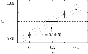
Figure 4: The speed of light squared, $c^{2}({\bf p})$, computed for an $\eta_{c}$ meson using the ASQTAD action with ${\bf p}=(p_{\mathrm{min}},p_{\mathrm{min}},0)$ and different Naik-term renormalizations $\epsilon$, where $p_{\mathrm{min}}$ is the smallest lattice momentum possible (approximately 500 MeV here). The correct value, $\epsilon=0.19(5)$, occurs at the intersection of the interpolating line with the line $c^{2}=1$, as shown. Here $am_{c}=.38$.

The HISQ results show even smaller $c^{2}$ errors on the fine lattices. Tuning to $\epsilon=-0.1155$, the tree-level value given by Eq. (20) for $am_{c}=0.43$, removes all errors in $c^{2}$ at the level of 1%. This suggests that one-loop and higher-order radiative corrections in $\epsilon$ are negligible for HISQ compared with the tree-level corrections. The dominance of tree-level contributions is confirmed by our HISQ analysis using the coarser lattice spacing, where $am_{c}\approx 0.66$. Here, we found the optimal value $\epsilon=-0.22(3)$ again by tuning $\epsilon$ until $c^{2}=1$ for a low-momentum $\eta_{c}$. (We overshot slightly and did simulations for $\epsilon=-0.21$ rather than $-0.22$.) Our tuned $\epsilon$ compares quite well with the tree-level prediction of $-0.246$ from Eq. (20). Consequently it is quite likely that the tree-level formula is sufficiently accurate for most practical applications today.

Note that setting $\epsilon=-1$ cancels out the Naik term completely. Tree-level errors are then order $a^{2}$ rather than order $a^{4}$, as in the HISQ action. Table 5 shows that these $a^{2}$ errors cause $c^{2}$ to be off by almost a factor of 2. This example underscores the importance of using $a^{2}$-improved actions in high-precision work.

On the coarse lattice, we use the $c^{2}({\bf p})$ with $p=p_{\mathrm{min}}$, the smallest nonzero momentum on our lattice, to tune $\epsilon$. It is important to verify that the tuned action gives the correct dispersion relation for other momenta as well. The data in Fig. 5 demonstrate that errors are less than a couple percent for meson momenta out to 1 GeV even on the coarse lattice where $am_{c}=0.66$. Indeed, the errors would probably have been smaller ($<1$%) had we tuned $\epsilon$ a little more accurately.

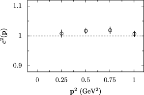
Figure 5: The speed of light squared, $c^{2}({\bf p}^{2})$, for $\eta_{c}$ mesons at different momenta on a lattice where $am_{c}\approx 0.66$ for the HISQ action with $\epsilon=-0.21$. A comparison with other results from Table 5 suggests that choosing $\epsilon=-0.22$ would move all points down onto the line $c^{2}=1$ to within errors.

We examined the spectrum of the $\psi$ meson family to further test the precision of our formalism. We used the $1/11$ fm lattices where $am_{c}\approx 0.4$, and therefore we expect errors of order 1–2% of the binding energy, or 5–10 MeV (see Section III.2). A particularly sensitive test is the hyperfine mass splitting between the $\psi$ and $\eta_{c}$. We tuned the bare $c$ mass until the mass of the local (and lightest) $\eta_{c}$ in our simulation agreed with experiment. Since there are no other free parameters in our action, the simulation then predicts a mass for the $\psi$. As is clear from Fig. 6, the $\psi$ mass in the simulation is quite accurate — certainly within the 5–10 MeV we expected.

The data shown in this last figure also bound taste-exchange errors. As shown there, different tastes of the $\eta_{c}$ have different masses, because of taste-exchange interactions. The maximum spread in the masses for the HISQ action, however, is only 9 MeV. This is much smaller than the spread from the ASQTAD action, where the splitting between, for example, the 0-link and 1-temporal-link pion masses is 40 MeV (compared to only 3 MeV for the same splitting with HISQ). (Uncorrected staggered quarks also show very large splittings japan-psi .) Note also that the spread in the $\psi$s is three times smaller than the spread in the $\eta_{c}$s. This is typical; the masses of mesons other than pseudoscalars are much less sensitive to taste-exchange effects.

The $\psi-\eta_{c}$ hyperfine splitting, for 0-link mesons in each case, is 109(3) MeV in our $1/11$ fm simulation with tuned $\epsilon$ ($=-0.115$). The 3% uncertainty is almost entirely due to tuning uncertainties in the lattice spacings since these uncertainties enter twice: once for converting the splitting from lattice to physical units, and once through uncertainties in the $c$ mass, which are themselves controlled by uncertainties in $a^{-1}$ nrqcd . Our HISQ result is somewhat smaller than the current experimental result of 117(1) MeV etac-data , but it needs three further corrections. (It is also worth noting that the current Particle Data Group average of 117 MeV is somewhat larger than the most recent experiments which find values in the range 113–115 MeV with uncertainties of 1–2 MeV; see etac-data .)

The first correction comes from the operators in Table 3 that must be added to the HISQ lagrangian in order to remove further discretization errors. Of these the most important for the hyperfine splitting is

$$\delta{\cal L}_{\mathrm{hfs}}=c_{\mathrm{hfs}}\,a^{2}m_{c}\,\overline{\psi}\sigma\cdot F\psi$$ (46)

where $c_{\mathrm{hfs}}={\cal O}(\alpha_{s})$. This will affect the hyperfine splitting in relative order $\alpha_{s}(am_{c})^{2}$, or at the level of $\pm 5$ MeV. The coefficient $c_{\mathrm{hfs}}$ is readily computed in perturbation theory and this calculation is underway.

The second correction comes from residual taste-exchange interactions, which from the data in Fig. 6 could be of order a few MeV. Both this error and that corrected by $\delta{\cal L}_{\mathrm{hfs}}$ are approximately proportional to $a^{2}$. So we can estimate them (together) by comparing to a calculation with a different lattice spacing. We repeated our hyperfine splitting analysis on the $1/8$ fm lattice using the tuned $\epsilon$ ($=-.21$). The $a^{2}$ errors should be a little more than twice as large on the coarser lattice since $a^{2}$ is almost exactly twice as large. We obtained a splitting of 110(3) MeV on the coarse lattice, which is essentially identical to the 109(3) MeV we obtained on the fine lattice. Combining these results, together with our a priori expectation of $\pm 5$ MeV errors from $a^{2}$ corrections, we obtain an $a^{2}$ corrected hyperfine splitting is 109(5) MeV.

The third correction is due to the fact that our simulation does not include effects from the annihilation of the valence $c\overline{c}$ quarks into two or more gluons. Such annihilations are responsible for small shifts in the $\eta_{c}$ and $\psi$ masses, as well as for the (non-electromagnetic) hadronic decay rate of each meson. The dominant contribution comes from $c\overline{c}\to gg$ and affects only the $\eta_{c}$. The shift in the $\eta_{c}$ energy is proportional to the perturbative amplitude for $c\overline{c}\to gg\to c\overline{c}$ at threshold bodwin-braaten-gpl and therefore positronium-result

$$\Delta E_{\eta_{c}}- i\,\Gamma(\eta_{c}\to\text{hadrons})/2$$ (47)

$$\propto\ln(2)-1-i\,\frac{\pi}{2}+{\cal O}(\alpha_{s}).$$

This result implies that the leading correction to the $\eta_{c}$ mass due to $c\overline{c}$ annihilation can be computed from the hadronic width:

$$\Delta E_{\eta_{c}} =\Gamma(\eta_{c}\to\text{hadrons})\left(\frac{\ln(2)-1}{\pi}+{\cal O}(\alpha_{s})\right)$$ (48)

$$=-2.4(8)\,\text{MeV}$$

where we use experimental results from etac-data . This correction increases our theoretical value for the $\psi$–$\eta_{c}$ splitting to 111(5) MeV, which agrees well with experiment. The sea-quark masses in our simulations are not quite correct, but both theoretical expectations and experience with previous simulations indicate that this has negligible effect on this hyperfine splitting.

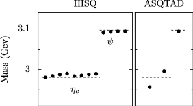
Figure 6: Masses for different tastes of the $\eta_{c}$ and $\psi$ using HISQ and ASQTAD $c$ quarks with $\epsilon=0$ on a $1/11$ fm lattice ($am_{c}\approx 0.4$). For HISQ, $\eta_{c}$s are given (from left to right) for the 0, 1, 2, and 3 spatial link tastes, without and then with a temporal link; only the spatial splittings are given for the $\psi$. For ASQTAD, $\eta_{c}$ results are given for only the 0-link and 1-temporal-link operators, and $\psi$ results for only the 0-link operator. The dashed lines indicate the results from experiment. Error bars are of order the size of the plot symbols.

This level of precision would be impossible using our ASQTAD results because the taste-exchange errors are tens of MeV — much larger than the $\pm 5$ MeV expected from other $a^{2}$ errors. This example confirms that taste-exchange errors are likely the dominant source of $a^{2}$ errors in the ASQTAD formalism. With HISQ, on the other hand, taste-exchange errors have been suppressed to a level commensurate with other errors.

Finally we also computed the masses of some radially and orbitally excited states in the $\psi$ family using HISQ, although not as accurately as the ground-state masses. High-precision determinations of excited-state masses require careful design of the meson sources and sinks used in the simulation. Here we did not attempt high precision, but rather used simple local sources to do a quick check on the spectrum. Our results, shown in Fig. 7, agree well with experiment to within our statistical errors.

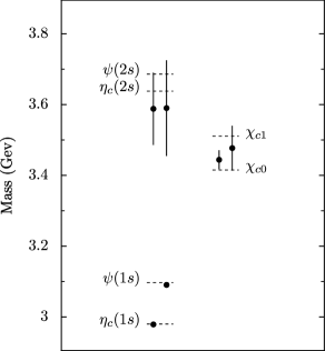
Figure 7: Masses for different excitations of the $\psi$ meson from a simulation at lattice spacing $1/11$ fm. The dashed lines indicate the results from experiment.

VI Simulation Techniques for Highly-Smeared Operators

It would be highly desirable to create new unquenched gluon configurations using the HISQ action in place of the ASQTAD action. The use of such configurations, with lattice spacings of order $a=0.1$ fm, would significantly reduce any residual worries about errors due to taste-exchange interactions.

Such simulations are complicated, however, by the heavily smeared, reunitarized links in the action. The additional smearing and reunitarization have no effect on the cost of the quark-matrix inversions required when updating gluon configurations, but they complicate calculation of the derivative $D_{a}(x,\mu)\,S_{q}$ of the quark action $S_{q}[U]$ with respect to an individual link operator $U_{\mu}(x)$. Derivative $D_{a}(x,\mu)$ is defined by

$$f(\mathrm{e}^{i\epsilon^{a}T^{a}}U_{\mu}(x))\equiv f(U_{\mu}(x))+\epsilon^{a}D_{a}(x,\mu)f(U_{\mu})+{\cal O}(\epsilon^{2})$$ (49)

for any function $f$ of $U_{\mu}(x)$. We developed and tested both an analytic and a stochastic version of the derivative for this action Follana:2003fe .

The analytic version employs a unitary projection

$$V\to(VV^{\dagger})^{-\frac{1}{2}}V$$ (50)

to reunitarize each smeared link $V$. The main obstacle is then computation of the gauge derivative of the inverse square root. Using the product-rule identity for the matrix $M\equiv VV^{\dagger}$,

$$M^{\frac{1}{2}}\left(DM^{-\frac{1}{2}}\right)+\left(DM^{-\frac{1}{2}}\right)M^{\frac{1}{2}}=-M^{-\frac{1}{2}}\left(DM\right)M^{-\frac{1}{2}},$$ (51)

we can solve for $D(VV^{\dagger})^{-\frac{1}{2}}$ directly, both iteratively by the conjugate gradient algorithm, and exactly by first diagonalizing $VV^{\dagger}$.

Using the chain rule, we combine $D(VV^{\dagger})^{-\frac{1}{2}}$ with standard derivatives of the base action and of the smeared links $V$. We encode derivatives of the action and smeared links generically, allowing for run-time changes independently in either. The additional cost of computing and combining $D(VV^{\dagger})^{-\frac{1}{2}}$ with these is minimal.

Several other analytic approaches have been developed for unitarized smearings Kamleh:2004xk ; Morningstar:2003gk . The authors of Kamleh:2004xk addressed the problem of computing the derivative of the matrix inverse square root by replacing it with a rational approximation. In Morningstar:2003gk , the smearing itself is unitary, explicitly avoiding the need to reunitarize and the inverse square root. In both, the derivatives are then computed straightforwardly.

In the stochastic approach, we define links

$$U^{\eta}_{\mu}(x)\equiv\mathrm{e}^{i\epsilon\eta(x,\mu)}U_{\mu}(x)$$ (52)

where $\eta(x,\mu)$ is now a field of traceless, hermitian $3\times 3$ random matrices, each with normalization

$$\langle\eta_{ij}\eta_{lm}\rangle_{\eta}=\left(\delta_{im}\delta_{jl}-\frac{1}{3}\delta_{ij}\delta_{lm}\right),$$ (53)

and $\epsilon$ is a very small number. Defining $\Delta S_{q}(x,\mu)$ to be the terms in $S_{q}[U^{\eta}]-S_{q}[U]$ containing $U_{\mu}(x)$, the derivative can be computed efficiently from

$$2\epsilon T^{a}D_{a}(x,\mu)\,S_{q}\approx\langle\eta(x,\mu)\,\Delta S_{q}(x,\mu)\rangle_{\eta}$$ (54)

averaged over a finite number of sets of random $\eta$s. Our numerical experiments suggest that 10–100 sets of $\eta$s are adequate for actions like HISQ. We will describe both our stochastic and analytic techniques in a later paper.

VII Conclusions

In this paper, we have demonstrated that taste-exchange interactions are perturbative and we have shown how to use Symanzik improvement to create a new staggered-quark action (HISQ) that has greatly reduced one-loop taste-exchange errors, no tree-level order $a^{2}$ errors, and no tree-level order $(am)^{4}$ errors to leading order in the quark’s velocity $v/c$. The HISQ action addresses one of the fundamental issues surrounding staggered-quark simulations by allowing us to estimate taste-exchange interactions through comparisons of HISQ with ASQTAD results. We presented numerical evidence that taste-exchange interactions in HISQ contribute less than 1% to light-quark quantities, like meson masses and decay constants, at lattice spacings as large as 0.1 fm.

The suppression of all order $(am)^{4}$ errors by powers of $(v/c)^{2}$ makes HISQ the most accurate discretization of the quark action for simulating $c$ quarks on current lattices. We demonstrated this with a new lattice QCD determination of the $\psi-\eta_{c}$ mass splitting, which agrees well with experiment. This result could be improved by computing the coefficient $c_{\mathrm{hfs}}$ in the correction $\delta{\cal L}_{\mathrm{hfs}}$ (Eq. (46)) to the HISQ action.

Our final HISQ action is defined by Eqs. (40–43). We showed that the tree-level value (Eq. (20)) for the Naik-term parameter $\epsilon$ is adequate at the level of 1% errors for lattice spacings at least as large as $1/8$ fm.

The HISQ formalism will be most useful for $D$ physics and works very well for such mesons. In Fig. 8, for example, we show the $D_{s}^{*}$–$D_{s}$ spin splitting from simulations with HISQ $c$ quarks using both our $1/8$ fm and $1/11$ fm lattices. As in the charmonium case, theory and experiment agree well here to within errors. Another very sensitive test of our simulations is to compare computed and experimental values for the mass difference $2m_{D_{s}}-m_{\eta_{c}}$, which is quite insensitive to tuning errors in the $c$ mass. We obtain 956(14) MeV using HISQ on the $1/11$ fm lattice, and 978(20) MeV on the $1/8$ fm lattice. Both values agree well with the splitting 956(1) MeV from experiment. Finally, we measured the speed of light and found $c^{2}=1.00(4)$ for the $D_{s}$ on the coarse lattice ($a=1/8$ fm with $\epsilon=-0.21$), confirming that the same coupling constant values work for both $D_{s}$ and $\eta_{c}$ mesons. It is important to appreciate that there are no free parameters available for tuning in the extraction of any of these results; all QCD parameters were tuned using other quantities.

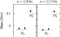
Figure 8: Masses for two different tastes of the $D_{s}$ and one for the $D_{s}^{*}$ using HISQ $c$ quarks on lattices with lattice spacings $a=1/8$ fm ($\epsilon=-0.21$) and $1/11$ fm ($\epsilon=-0.115$). For HISQ, $D_{s}$s are given (from left to right) for the 0-link and 1-temporal-link mesons; only the 0-link splitting is given for the $D_{s}^{*}$. The dashed lines indicate the results from experiment. The error bars shown are from the simulated values for $m_{D_{s}}-m_{\eta_{c}}/2$ and $m_{D_{s}^{*}}-m_{\eta_{c}}/2$, since these quantities are insensitive to the $c$ mass and the $c$ mass was tuned to make the simulated value for $m_{\eta_{c}}$ exact.

As we will discuss in a later paper, the HISQ formalism is particularly useful for accurate calculations of quantities like $f_{D}$, $f_{D_{s}}$, $D\to\pi l\nu$, and so on. These all require currents and these currents, even though they are conserved or partially conserved, have order $\alpha_{s}(am)^{2}$ renormalizations. Consider, for example, $c\overline{c}$ annihilation into a (virtual) photon. The electromagnetic current can be computed by inserting photon link operators,

$$U^{\mathrm{QED}}_{\mu}\equiv\exp\left(-ie_{q}\int_{x}^{x+\hat{\mu}}dx\cdot A^{\mathrm{QED}}\right),$$ (55)

into the HISQ action and then expanding to first order in $A^{\mathrm{QED}}$ to obtain

$$-ie_{q}\,A_{\mu}^{\mathrm{QED}}\,J_{\mu}^{\mathrm{QED}}.$$ (56)

Current $J^{\mathrm{QED}}$ is not renormalized, because of QED’s gauge symmetry, but it is not the only operator that contributes to $c\overline{c}$ annihilation. In addition there are ${\cal O}(a^{2})$ correction terms that contribute,

$$\begin{split}c_{1}\,\alpha_{s}\,a^{2}m\,\overline{\psi}&\,\sigma\cdot eF^{\mathrm{QED}}\,\psi\\ &+c_{2}\,\alpha_{s}\,a^{2}\,\overline{\psi}\,(D\cdot eF)^{\mathrm{QED}}\cdot\gamma\,\psi,\end{split}$$ (57)

just as for the gluon fields. The first correction term renormalizes the quark’s magnetic moment, the second its charge radius. Such terms are normally negligible since the extra derivatives introduce extra powers of $(ap)^{2}$ and $p$ is small. For $c$ quark annihilations, however, the extra derivatives become $c$ quark masses instead of small momenta, and so are more important. It is easy to compute coefficients $c_{1}$ and $c_{2}$ in perturbation theory, but contributions to annihilation from these operators are indistinguishable from those coming from the leading operator $J^{\mathrm{QED}}$. Consequently we can omit the corrections and, instead, introduce a renormalization constant for $J^{\mathrm{QED}}$:

$$J_{\mu}^{\mathrm{QED,continuum}}=Z_{\mathrm{eff}}\,J^{\mathrm{QED},\mathrm{HISQ}}_{\mu}$$ (58)

where

$$Z_{\mathrm{eff}}=1+c\,\alpha_{s}\,(am)^{2}+{\cal O}(\alpha_{s}^{2}\,(am)^{2}).$$ (59)

The situation is very similar for (partially-conserved) weak-interaction currents. Again the current derived from the action requires ${\cal O}(\alpha_{s}(am)^{2})$ corrections. Once these one-loop corrections have been calculated and included, however, the remaining terms are only ${\cal O}(\alpha_{s}^{2}(am)^{2})$. Consequently one-loop radiative corrections are all that is necessary to achieve 1–2% precision for $f_{D}$, $D\to\pi l\nu$, and similar quantities. Other discretization errors in these quantities should be of order 1% or less. With one-loop renormalizations, lattice results will be more accurate than current results from CLEO-c and the $b$ factories.

Appendix A Gamma Matrices

The complete set of spinor matrices can be labeled by a four-component vector $n_{\mu}$ consisting of 0s and 1s (i.e., $n_{\mu}\in\mathbb{Z}_{2}$):

$$\gamma_{n}\,\equiv\,\prod_{\mu=0}^{3}(\gamma_{\mu})^{n_{\mu}}.$$ (60)

We will also sometimes use the more conventional, but equivalent (up to a phase) hermitian set:

$$1,\quad\gamma_{5}\equiv\gamma_{t}\gamma_{x}\gamma_{y}\gamma_{z},\quad\gamma_{\mu},$$

$$\quad\gamma_{5\mu}\equiv i\gamma_{5}\gamma_{\mu},\quad\gamma_{\mu\nu}\equiv\mbox{$\frac{i}{2}$}[\gamma_{\mu},\gamma_{\nu}].$$ (61)

The $\gamma_{n}$s have several useful properties:

• orthonormal:

  $${\rm\,Tr\,}(\gamma_{n}^{\dagger}\gamma_{m})=4\,\delta_{nm}$$ (62)

• closed under multiplication:

  $$\gamma_{n}\gamma_{m}=(-1)^{n\cdot m^{<}}\,\gamma_{n+m}$$ (63)

  where

  $$m_{\mu}^{<}\equiv\sum_{\nu<\mu}m_{\nu}\bmod 2$$ (64)

  and

  $$n\cdot m^{<}=n^{>}\cdot m$$ (65)

  with

  $$n^{>}_{\mu}\equiv\sum_{\nu>\mu}n_{\nu}\bmod 2;$$ (66)

• hermitian or antihermitian:

  $$\gamma_{n}^{\dagger}=(-1)^{n\cdot n^{<}}\,\gamma_{n}=\gamma_{n}^{-1};$$ (67)

• commuting or anticommuting:

  $$\gamma_{n}\,\gamma_{m}=(-1)^{\overline{m}\cdot n}\,\gamma_{m}\,\gamma_{n}$$ (68)

  where

  $$\overline{m}_{\mu} \equiv m^{>}_{\mu}+m^{<}_{\mu}=\sum_{\nu\neq\mu}m_{\nu}\bmod 2$$ (69)

  $$= \begin{cases}m_{\mu}&\text{if $m^{2}$ even}\cr(m_{\mu}+1)\bmod 2&\text{if $m^{2}$ odd,}\cr\end{cases}$$

  and

  $$\overline{m}\cdot n=\overline{n}\cdot m,$$ (70)

  $$\overline{\overline{m}}=m\qquad(\overline{m}\cdot m)\bmod 2=0;$$ (71)

• permutation operator: if one uses the standard representation for gamma matrices, where

  $$\gamma_{0}=\left(\begin{array}[]{cc}1&0\\ 0&-1\end{array}\right)\quad\quad\gamma_{i}=\left(\begin{array}[]{cc}0&\sigma_{i}\\ \sigma_{i}&0\end{array}\right)$$ (72)

  and

  $$\sigma_{1}=\left(\begin{array}[]{cc}0&1\\ 1&0\end{array}\right)\quad\quad\sigma_{2}=\left(\begin{array}[]{cc}0&-i\\ i&0\end{array}\right)\quad\quad$$ (77)

  $$\sigma_{3}=\left(\begin{array}[]{cc}1&0\\ 0&-1\end{array}\right),$$ (80)

  then there is at most one nonzero element in any row or any column of any $\gamma_{n}$, and that element is $\pm 1$ or $\pm i$. Thus multiplying a spinor $\psi$ by $\gamma_{n}$ simply permutes the spinor components of $\psi$, multiplying each by $\pm 1$ or $\pm i$.

A convenient notation, reminiscent of $\gamma_{5\mu}$, is

$$\gamma_{nm}\equiv\gamma_{n}\,\gamma_{m}.$$ (81)

Appendix B Staggered Quarks

The naive discretization of the quark action is formally equivalent to the staggered-quark discretization. Staggering is an important optimization in simulations; it is also a remarkable property. Consider the following local transformation of the naive-quark field:

$$\psi(x)\to\Omega(x)\,\chi(x)\quad\quad\overline{\psi}(x)\to\overline{\chi}(x)\,\Omega^{\dagger}(x)$$ (82)

where

$$\Omega(x)\equiv\gamma_{x}\equiv\prod_{\mu=0}^{3}(\gamma_{\mu})^{x_{\mu}},$$ (83)

and we have set the lattice spacing $a=1$ for convenience. (We will use lattice units, where $a=1$, in this and all succeeding appendices.) Note that

$$\Omega(x)=\gamma_{n}\quad\quad\text{for ${n_{\mu}=x_{\mu}\,\bmod\,2}$;}$$ (84)

there are only 16 different $\Omega$s. It is easy to show that

$$\alpha_{\mu}(x) \equiv \Omega^{\dagger}(x)\gamma_{\mu}\Omega(x\pm\hat{\mu})\,=\,(-1)^{x^{<}_{\mu}},$$ (85)

$$1 = \Omega^{\dagger}(x)\Omega(x)$$ (86)

where $x^{<}_{\mu}\equiv x_{0}+x_{1}+\cdots+x_{\mu-1}$ (see Appendix A). Therefore the naive-quark action can be rewritten

$$\overline{\psi}(x)(\gamma\cdot\Delta+m)\psi(x)\,=\,\overline{\chi}(x)(\alpha(x)\cdot\Delta+m)\chi(x).$$ (87)

Remarkably the $\chi$ action is diagonal in spinor space; each component of $\chi$ is exactly equivalent to every other component. Consequently the $\chi$ propagator is diagonal in spinor space in any background gauge field:

$$\langle\chi(x)\overline{\chi}(y)\rangle_{\chi}\,=\,s(x,y)\,{\bf 1}_{\rm spinor}$$ (88)

where $s(x,y)$ is the one-spinor-component staggered-quark propagator. Transforming back to the original naive-quark field we find that

$$S_{F}\,\equiv\,\langle\psi(x)\overline{\psi}(y)\rangle_{\psi}\,=\,s(x,y)\,\Omega(x)\Omega^{\dagger}(y).$$ (89)

This last result is a somewhat surprising consequence of the doubling symmetry. It says that the spinor structure of the naive-quark propagator is completely independent of the gauge field. This is certainly not the case for individual tastes of naive quark, whose spins will flip back and forth as they scatter off fluctuations in the chromomagnetic field, for example. The sixteen tastes of the naive quark field are packaged in such a way, however, that all gauge-field dependence vanishes in the spinor structure.

Doubling symmetry is immediately evident in the staggered action, Eq. (87), since the action is invariant under

$$\chi(x)\to{\cal B}_{\zeta}(0)\,\chi(x),$$ (90)

which merely scrambles the (equivalent) spinor components of $\chi(x)$, and since

$${\cal B}_{\zeta}(x)\,\Omega(x)=\Omega(x)\,{\cal B}_{\zeta}(0).$$ (91)

In simulations one generally discards all but one spinor component of $\chi(x)$, resulting in highly efficient algorithms. The Symanzik improvements discussed above are trivially incorporated.

Note, finally, that Eq. (91) implies

$${\cal B}_{\zeta}(x)\,\Omega(x)\Omega^{\dagger}(y)\,{\cal B}_{\zeta}^{\dagger}(y)\,=\,\Omega(x)\Omega^{\dagger}(y).$$ (92)

and therefore the naive-quark propagator, $S_{F}$, satisfies

$$S_{F}(x,y)\,=\,{\cal B}_{\zeta}(x)\,S_{F}(x,y)\,{\cal B}_{\zeta}^{\dagger}(y)$$ (93)

for any background gauge field. In momentum space this becomes

$$S_{F}(p,q)\,=\,{\cal B}_{\zeta}(0)\,S_{F}(p\!+\!\zeta\pi,q\!+\!\zeta\pi)\,{\cal B}_{\zeta}^{\dagger}(0),$$ (94)

which is an exact relationship that is useful in perturbative calculations. This last relation, which is easily checked at tree level (but true to all orders in $\alpha_{s}$), shows that there is only one sixteenth as much information in the naive-quark propagator as naively expected.

Appendix C Taste, Naive vs. Staggered

The quark field $\psi(x)$ will typically contain contributions from all 16 tastes. One can separate out (approximately) the different tastes by blocking the field on hypercubes that have two sites per side. One way to project out the $\zeta=0$ taste, for example, is to average over the hypercube:

$$\psi_{B}=\frac{1}{16}\sum_{\delta x_{\mu}\in\mathbb{Z}_{2}}\psi(x_{B}+\delta x)$$ (95)

where $x_{B}$, with $x_{B\mu}\bmod 2=0$, identifies the hypercube, and the sum is over all 16 sites in the hypercube. Any component of $\psi(x)$ that has momentum $p\approx\zeta\pi$ with $\zeta\neq 0$ will be strongly suppressed by the average. (The suppression is ${\cal O}(a^{2}p^{2})$ for a mode with momentum $p+\zeta\pi$.) A $\zeta\neq 0$ piece of $\psi(x)$ can be isolated by applying a doubling operator ${\cal B}_{\zeta}$ to transform that component to $\zeta=0$, and then, again, averaging over the hypercube to isolate that component:

$$\psi_{B}^{(\zeta)}=\frac{1}{16}\sum_{\delta x_{\mu}\in\mathbb{Z}_{2}}{\cal B}_{\zeta}(x_{B}+\delta x)\,\psi(x_{B}+\delta x).$$ (96)

The 16 blocked fields $\psi_{B}^{(\zeta)}$, with one for each $\zeta$, describe the 16 different tastes of quark, each now in the low momentum sector (i.e., with $p_{\mu}\leq\pi/2$).

With staggered quarks, one keeps only one component of $\chi(x)$ since the components are equivalent and decouple:

$$\chi(x)\to\left[\begin{array}[]{c}\chi_{1}(x)\\ 0\\ 0\\ 0\end{array}\right].$$ (97)

We can use our hypercube blocking (Eq. (96)) to translate this single field back into blocked fields for “ordinary” quarks of different tastes $\zeta$:

$$\begin{split}\sum_{{\delta x}_{\mu}\in\mathbb{Z}_{2}}&{\cal B}_{\zeta}(x_{B}+{\delta x})\,\psi(x_{B}+{\delta x})\\ =&\sum_{\delta x}\Omega({\delta x})\,{\cal B}_{\zeta}(0)\left[\begin{array}[]{c}\chi_{1}(x_{B}+{\delta x})\\ 0\\ 0\\ 0\end{array}\right].\end{split}$$ (98)

Only four of the sixteen blocked fields are independent, however, because ${\cal B}_{\zeta}(0)\,\chi(x)$ is always proportional to one of only four different spinors:

$$\left[\begin{array}[]{c}\chi_{1}(x)\\ 0\\ 0\\ 0\end{array}\right],\>\left[\begin{array}[]{c}0\\ \chi_{1}(x)\\ 0\\ 0\end{array}\right],\>\left[\begin{array}[]{c}0\\ 0\\ \chi_{1}(x)\\ 0\end{array}\right],\>\left[\begin{array}[]{c}0\\ 0\\ 0\\ \chi_{1}(x)\end{array}\right].$$ (99)

(This is because ${\cal B}_{\zeta}(0)=\gamma_{\overline{\zeta}}$ and all $\gamma_{n}$s when applied to a spinor merely permute the elements of the spinor, multiplying each by $\pm 1$ or $\pm i$.) Consequently we can reconstruct just four tastes, $t=1\ldots 4$, of blocked quark from a single staggered field:

$$\tilde{\psi}_{B}^{(t)}=\sum_{\delta x}\Omega({\delta x})\,\hat{\chi}^{(t)}\,\chi_{1}(x_{B}+{\delta x})$$ (100)

where the $\hat{\chi}^{(t)}$ are unit spinors with $\hat{\chi}^{(t)}_{i}=\delta_{i,t}$.

This last formula defines the standard taste basis for staggered quarks. It is of more use conceptually than practically, and we will not need it in what follows.

Formula (98) shows that some $\zeta$’s become indistinguishable in the staggered approximation. In fact, by explicit calculation (given our specific representation of the $\gamma$ matrices), one finds that the $\zeta$s fall into four equivalence classes composed of indistinguishable $\zeta$s:

$$A: 0000\quad 0001\quad 0110\quad 0111$$

$$B: 0010\quad 0011\quad 0100\quad 0101$$

$$C: 1000\quad 1001\quad 1110\quad 1111$$

$$D: 1010\quad 1011\quad 1100\quad 1101$$ (101)

These four classes correspond to the four tastes of staggered quark; all the $\zeta$s in a single class give the same staggered-quark field $\tilde{\psi}_{B}^{(t)}$ (Eq. (100)) from Eq. (98).

The equivalence of the $\zeta$s within a single class is preserved under addition of $\zeta$s: for example, adding any two $\zeta$s from class $B$ always gives a $\zeta$ in class $A$, while adding any vector from class $B$ to any vector from class $C$ always gives a vector in class $D$. The full addition table for these classes is:

$+$	$A$	$B$	$C$	$D$
$A$	$A$	$B$	$C$	$D$
$B$	$B$	$A$	$D$	$C$
$C$	$C$	$D$	$A$	$B$
$D$	$D$	$C$	$B$	$A$

This kind of structure is necessary for the four-fold reduction in the number of tastes due to staggering — that is, 16 tastes of naive quark are reduced to 4 tastes of staggered quark because we can consistently identify certain corners of the Brillouin zone with each other in the staggered case.

Appendix D Naive-Quark Currents

Naive quarks lead to huge numbers of nearly equivalent mesons. Where in ordinary QCD one might consider a single meson operator, $J_{n}=\overline{\psi}\gamma_{n}\psi$, one has 16 point-split operators in the naive theory each of which couples to a different meson:

$$J_{n}^{(s)}(x) \equiv \overline{\psi}(x)\,\gamma_{n}^{(s)}\,\psi(x)$$ (102)

$$\equiv \overline{\psi}(x)\,\gamma_{n}\,\psi(x+\delta x_{sn})$$

$$\propto \overline{\chi}(x)\,\gamma_{s}\,\chi(x+\delta x_{sn}),$$

where $s$ is any one of the 16 four-vectors consisting of 0s and 1s only,

$$\delta x_{sn}\equiv(s+n)\,\bmod\,2,$$ (103)

and link operators $U_{\mu}$ are implicit (and $a=1$ still). Each of these operators creates a different version of the $J_{n}$ meson; they are orthogonal. This is because

$$J_{n}^{(s)}\,\to\,(-1)^{s_{\mu}}\,J_{n}^{(s)}$$ (104)

under a doubling transformation where

$$\psi(x)\,\to\,{\cal B}_{\zeta=\hat{\mu}}(x)\,\psi(x)\qquad\overline{\psi}(x)\,\to\,\overline{\psi}(x){\cal B}_{\hat{\mu}}^{\dagger}(x).$$ (105)

Thus the four-vector $s$ determines the bilinear’s transformation properties under arbitrary doubling transformations; it specifies the bilinear’s “signature” under doubling transformations. Since doubling transformations are symmetries of the naive theory, the doubling signature is conserved: for example,

$$\langle\,J_{m}^{(r)}\,\,J_{n}^{(s)\dagger}\,\rangle\,=\,0\quad\quad\mbox{if $r\neq s$},$$ (106)

which proves that each of our point splittings creates a different meson.

Different signatures correspond to different variations of the same continuum meson, typically with slightly different masses, etc. These are the different tastes of the meson. We label different tastes by the corresponding signature $s$ in the meson’s rest frame.

Additional mesons are made by boosting particles into other corners of the Brillouin zone:

$$p_{\mathrm{tot}}\approx\zeta\pi$$ (107)

for one of the sixteen $\zeta$s. Such mesons would be highly relativistic in the continuum, but here they are equivalent to low-energy mesons because of the doubling symmetry: for example, the antiquark in the meson might carry a momentum near zero, while the quark carries $\zeta\pi$ but is then equivalent to a zero-momentum quark state through the doubling symmetry. Pushing such momenta through a naive-quark bilinear, using for example

$$\sum_{x}\mathrm{e}^{i\,p_{\mathrm{tot}}\cdot x}\,J^{(s)}_{n}(x),$$ (108)

changes the quantum numbers of the meson created by the operator. To see this, consider current

$$J_{n}^{(\zeta,s)}(x) \equiv (-1)^{\zeta\cdot x}\,\overline{\psi}(x)\,\gamma_{\,\overline{\zeta}}^{\dagger}\,\gamma_{n}^{(s)}\,\psi(x)$$ (109)

$$= \overline{\psi}(x)\,{\cal B}_{\zeta}^{\dagger}(x)\,\gamma_{n}^{(s)}\,\psi(x)\rule{0.0pt}{12.91663pt}$$

$$\propto \overline{\chi}(x)\,\gamma_{\,\overline{\zeta}}^{\dagger}\,\gamma_{s}\,\chi(x+\delta x_{sn})\rule{0.0pt}{12.91663pt}$$ (110)

which has signature $(\overline{\zeta}+s)\bmod 2$. This current obviously carries momentum $p_{\mathrm{tot}}=\zeta\pi$ if averaged over all $x$. It is easy to show that flavor-nonsinglet mesons created by $J_{n}^{(\zeta,s)}$ with different $\zeta$s are all identical, and therefore all carry taste $s$. For a $\overline{u}d$ meson, for example, we can use the separate doubling symmetries of the $u$ and $d$ to prove that

$$\langle\,J_{n}^{(\zeta,s)}(x)\,J_{n}^{(\zeta,s)\dagger}(y)\,\rangle \equiv \langle\,\overline{u}{\cal B}_{\zeta}^{\dagger}\gamma_{n}^{(s)}d\,\,\overline{d}\gamma_{n}^{(s)}{\cal B}_{\zeta}u\,\rangle$$ (111)

$$= \langle\,\overline{u}\gamma_{n}^{(s)}d\,\,\overline{d}\gamma_{n}^{(s)}u\,\rangle\rule{0.0pt}{12.91663pt}$$

$$\equiv \langle\,J_{n}^{(s)}(x)\,J_{n}^{(s)\dagger}(y)\,\rangle\rule{0.0pt}{12.91663pt}$$

for all $\zeta$s.

The labeling on $J_{n}^{(\zeta,s)}$ is intuitive (and therefore useful) only if the current is averaged over $x$ in such a way that $p_{\mathrm{tot}}=\zeta\pi+p$ where $-\pi/2<p_{\mu}\leq\pi/2$ for all $\mu$; the combination of all $\zeta$s and $p$s covers all of momentum space, so nothing is lost by this restriction and double counting is avoided. We can enforce this restriction on the momenta by redefining the current on a blocked lattice with one site at the center of every $2^{4}$ hypercube on the original lattice, just as we did for the quark field (Section C):

$$J_{Bn}^{(\zeta,s)}\equiv\sum_{\delta x_{\mu}\in\mathbb{Z}_{2}}J_{n}^{(\zeta,s)}(x_{B}+\delta x)$$ (112)

where $x_{B}$ identifies the hypercube (with $x_{B\mu}\bmod 2=0$). The blocked current creates a meson of taste $s$ with momentum in the $\zeta\pi$ corner of the Brillouin zone.

Note that momentum and taste conservation imply

$$\sum_{x,y}\langle\,J_{n}^{(\zeta,s)}(x)\,J_{n}^{(\zeta^{\prime},s^{\prime})\dagger}(y)\,\rangle\,=\,0$$ (113)

unless $\zeta=\zeta^{\prime}$ and $s=s^{\prime}$. Consequently the different operators are orthogonal when analyzed in momentum space. Typically we sum over space, however, but not time. In that case operators with the same signature, but where $\zeta^{\prime}-\zeta=\pm\hat{t}$, can mix. This mixing leads to components in meson propagators that oscillate in time, as we discuss below.

To summarize, there are 16 sets, each set labeled by taste $s$, of 16 identical mesons, each meson labeled by $\zeta$, for each flavor-nonsinglet meson in the continuum. Each corner $\zeta$ of the Brillouin zone has a single representative of each taste of meson.

Flavor-singlet mesons are slightly more complicated. In a $\overline{u}u$ meson, for example, the quark and antiquark are created by the same field, and so do not have separate doubling transformations. Therefore the argument relating $J_{n}^{(\zeta,s)}$s with different $\zeta$s doesn’t work. The only contributions that spoil this argument are from annihilation, where the meson’s quark and antiquark annihilate into gluons. Annihilation gluons that contribute to, for example,

$$\sum_{\vec{x}}\langle\,J_{n}^{(\zeta,s)}(x)\,J_{n}^{(\zeta,s)\dagger}(0)\,\rangle$$ (114)

carry total momentum $\zeta\pi$ and so are far off-shell unless $\zeta=0$. This has two implications: First, annihilation contributions will be different for different $\zeta$s. And, second, only the $\zeta=0$ case has the correct coupling between the flavor-singlet quarks and purely gluonic channels. In fact, only the taste-singlet state, among the $\zeta=0$ states, couples to the gluons since

$$\langle\,J_{n}^{(s)}(x)\,\rangle_{\psi} \propto {\rm\,Tr\,}(\gamma_{s})$$ (115)

$$= 0\quad\quad\mbox{unless $s=0$}.$$

A similar condition applies to nonzero $\zeta$s as well. For each $\zeta$ there is only one taste that can couple to gluons. The gluons are highly virtual if $\zeta$ is nonzero. These last contributions are taste-violating because they change quark taste along quark lines; they are removed by the contact terms discussed in this paper.

It is not surprising that the flavor-singlet mesons are more complicated. They usually have to be, particularly in the pseudoscalar channel where the $U(1)$ problem must be resolved. In our naive-quark theory, only the $\zeta=s=0$ mesons couple properly to gluons. The masses of pseudoscalars with $\zeta=s=0$ are shifted properly by instantons in the chiral limit, so that the $U(1)$ problem is resolved. The $\zeta=s=0$ neutral pion is also the only pion that decays to two photons. The corresponding axial-vector current is only approximately conserved, even in the chiral limit, so anomalies are not needed to mediate the photon decay.

Appendix E Staggered-Quark Currents

The 256 different mesons created by the naive-quark bilinears $J_{n}^{(\zeta,s)}$ include 16 identical copies of each distinct taste of meson. Staggering the quark fields discards identical copies, leaving just 16 distinct tastes. The naive-quark bilinears corresponding to the staggered-quark bilinears are the ones that become diagonal after they are staggered. Any other operator creates mesons that mix different spinor components of the staggered quark operator $\chi(x)$ (Eq. (82)), and so is discarded when we stagger.

We can identify the bilinears that survive staggering by noting that

$$J^{(\zeta,s)}_{n} \propto \overline{\chi}\,\gamma_{\,\overline{\zeta}}^{\dagger}\,\gamma_{s}\,\chi$$ (116)

$$\to \overline{\chi}\,\chi$$

after staggering provided $\zeta=\overline{s}$. The staggered-quark operator is therefore

$$J_{n}^{(\overline{s},s)} \equiv {(-1)^{\overline{s}\cdot x}}\,\,\overline{\psi}(x)\,\gamma_{s}^{\dagger}\,\gamma_{n}\,\psi(x+\delta x_{sn})$$ (117)

$$= \beta_{n}^{(s)}(x)\,\,\overline{\chi}(x)\,\chi(x+\delta x_{sn})$$

where again $\delta x_{sn}=(s+n)\bmod 2$ (with $a=1$), and

$$\beta_{n}^{(s)}(x) =\mbox{$\frac{1}{4}$}\,{\rm\,Tr\,}\left(\gamma^{\dagger}_{s}\gamma^{\dagger}_{x}\gamma_{n}\gamma_{x+s+n}\right)$$ (118)

$$=(-1)^{x\cdot(s^{<}+n^{>})}\,(-1)^{n\cdot(s+n)^{<}}.$$

Each taste $s$ in the staggered theory corresponds to a specific corner of the Brillouin zone, with $p_{\mathrm{tot}}\approx\overline{s}\pi$, in the naive-quark theory. These operators have zero signature and so are unchanged under doubling transformations (Eq. (6)).

It is useful for formal analyses, though less so for simulations, to introduce a slightly different definition for these bilinears by defining a new operator on our naive-quark field:

$$\gamma_{n}\otimes\xi_{s}\,\psi(x)\,\equiv\,(-1)^{\overline{s}\cdot x}\,\gamma_{s}^{\dagger}\,\gamma_{n}\,\psi(x\oplus(n+s)),$$ (119)

where $\oplus$ adds vector $n+s$ to $x$ “modulo” the hypercube that $x$ lies in — that is,

$$(x\oplus n)_{\mu}\equiv x_{B\mu}+(x_{\mu}-x_{B\mu}+n_{\mu})\bmod 2$$ (120)

when $x$ is in the hypercube labeled by site $x_{B}$ (with $x_{B\mu}\bmod 2=0$). Thus $x\oplus n$ is in the same hypercube as $x$. With this definition, we can redefine the staggered-quark current with spin $n$ and taste $s$ to be:

$$\overline{\psi}(x)\,\gamma_{n}\otimes\xi_{s}\,\psi(x).$$ (121)

The $\oplus$ means that the new operators $\gamma_{n}\otimes\xi_{s}$ have a simple algebra. If, for example,

$$\tilde{\psi}(x)\equiv\gamma_{n}\otimes\xi_{s}\,\psi(x)$$ (122)

then, using Eq. (68),

$$\gamma_{m}\otimes\xi_{r}\,\tilde{\psi}(x)=\gamma_{m}\gamma_{n}\otimes\xi_{r}\xi_{s}\,\psi(x),$$ (123)

which implies that in general

$$\gamma_{m}\otimes\xi_{r}\,\,\gamma_{n}\otimes\xi_{s}\,\,=\,\,\gamma_{m}\gamma_{n}\otimes\xi_{r}\xi_{s}.$$ (124)

Note that these definitions also imply that $\xi$s anticommute just as $\gamma$s: for example,

$$\gamma_{n}\otimes\xi_{r}\xi_{s}=(-1)^{\overline{r}\cdot s}\,\gamma_{n}\otimes\xi_{s}\xi_{r}.$$ (125)

We can effectively restrict our current to the $\zeta=\overline{s}$ corner of the Brillouin zone by again blocking on $2^{4}$ hypercubes to obtain

$${\cal J}^{(n)}_{s}(x_{B})=\frac{1}{16}\sum_{\delta x_{\mu}\in\mathbb{Z}_{2}}\overline{\psi}(x_{B}+\delta x)\,\gamma_{n}\otimes\xi_{s}\,\psi(x_{B}+\delta x)$$ (126)

where $x_{B\mu}\bmod 2=0$. This formula is related to a more standard formula by staggering the meson operator:

$$\begin{split}\overline{\psi}(x)\,\gamma_{n}&\otimes\xi_{s}\,\psi(x)\\ &=\overline{\chi}(x)\,\gamma_{s}^{\dagger}\gamma_{x}^{\dagger}\,\gamma_{n}\,\gamma_{x+\delta x_{sn}}\,\chi(x\oplus\delta x_{sn})\end{split}$$ (127)

where the shift $\delta x_{sn}$ guarantees that the product of $\gamma$s is proportional to the unit matrix. We can rewrite this in terms of a sum over $\delta x$s in the positive unit hypercube:

$$\sum_{\delta x_{\mu}\in\mathbb{Z}_{2}}\overline{\chi}(x)\,\mbox{$\frac{1}{4}$}{\rm\,Tr\,}\left(\gamma^{\dagger}_{s}\,\gamma^{\dagger}_{x}\,\gamma_{n}\,\gamma_{x+\delta x}\right)\,\chi(x\oplus\delta x).$$ (128)

Averaging over the hypercube gives a standard formula for ${\cal J}^{(n)}_{s}$:

$$\frac{1}{16}\sum_{\delta x,\delta x^{\prime}}\overline{\chi}(x_{B}+\delta x)\mbox{$\frac{1}{4}$}{\rm\,Tr\,}\left(\gamma^{\dagger}_{s}\,\gamma^{\dagger}_{\delta x}\,\gamma_{n}\,\gamma_{\delta x^{\prime}}\right)\,\chi(x_{B}+\delta x^{\prime}).$$ (129)

Taste and spinor structure in $\overline{\psi}(x)\gamma_{n}\otimes\xi_{s}\psi(x)$ are both described by the same kind of four vector consisting of 0s and 1s. For this reason it is common practice to use the same terminology for describing taste as we do for spinor structure. Thus, for example, $\overline{\psi}(x)\,\gamma_{5}\otimes\xi_{5}\,\psi(x)$ creates a pseudoscalar meson with “pseudoscalar taste.” In this case $n=s=(1,1,1,1)$, and, from Eq. (117),

$$\overline{\psi}(x)\,\gamma_{5}\otimes\xi_{5}\,\psi(x) = \beta_{5}^{(5)}(x)\,\overline{\chi}(x)\chi(x)$$ (130)

$$= (-1)^{x\cdot x}\,\overline{\chi}(x)\chi(x).$$

A different pion is created by $\overline{\psi}(x)\gamma_{5}\otimes\xi_{5\mu}\psi(x)$, this one with axial-vector taste:

$$\overline{\psi}(x)\,\gamma_{5}\otimes\xi_{5\mu}\,\psi(x)=\beta_{5}^{(5\mu)}(x)\,\overline{\chi}(x)\chi(x\oplus\hat{\mu}).$$ (131)

The pion created by this operator is sometimes called a $5\otimes 5\mu$ or “1-link pion” since the operator is split by one link or lattice spacing. Similarly $\overline{\psi}(x)\gamma_{5}\otimes\xi_{5}\psi(x)$ creates a $5\otimes 5$ or 0-link pion.

Other naive-quark operators can be recast in terms of the spinor/taste operators. For example, the naive-quark action has a chiral symmetry in the massless limit under transformations

$$\psi(x) \to \exp(i\,\theta\,\gamma_{5}\otimes\xi_{5})\,\psi(x)$$

$$\overline{\psi}(x) \to \overline{\psi}(x)\,\exp(i\,\theta\,\gamma_{5}\otimes\xi_{5}),$$ (132)

where the $\xi_{5}$s express the fact that the symmetry operation does not translate (move) $\psi(x)$.

Appendix F One Loop Taste-Changing

The Symanzik procedure for removing ${\cal O}(a^{2})$ one-loop taste-exchange effects from the ASQTAD action involves two steps: 1) we compute taste-changing amplitudes for $q\overline{q}\to q\overline{q}$ with massless quarks in one-loop order using lattice perturbation theory; and 2) we design local taste-changing counterterms for the staggered-quark action that cancel these one-loop amplitudes. We find it easiest to work with the naive-quark theory, converting to staggered quarks only at the end.

In order $a^{2}$ we need only consider quarks at threshold — that is, quarks with momentum $p=\pm\zeta\pi$ for one of the sixteen $\zeta$’s with $\zeta_{\mu}\in\mathbb{Z}_{2}$ (where, again, $a=1$). Taste-changing amplitudes are ones where the incoming and outgoing momenta along any particular quark line differ by $\zeta\pi$ for one of the $\zeta$s. For $q\overline{q}\to q\overline{q}$, overall momentum conservation demands that the opposite change occur along the other quark line. Consequently while taste changes along individual quark lines, total taste is conserved. It is enough to compute amplitudes $A(0,0;\zeta\pi,-\zeta\pi)$ where the initial quarks have zero momentum and the final quarks have momenta $\zeta\pi$ for any $\zeta$. (Recall that $\zeta\pi$ and $-\zeta\pi$ are the same momentum on the lattice.) Amplitudes with other quark tastes in the initial state are related to these amplitudes by applying the doubling symmetry to each quark line separately:

$$A(\zeta^{\prime}\pi,\zeta^{\prime\prime}\pi;(\zeta^{\prime}+\zeta)\pi,(\zeta^{\prime\prime}-\zeta)\pi)=A(0,0;\zeta\pi,-\zeta\pi)$$ (133)

where $\zeta^{\prime}_{\mu},\zeta^{\prime\prime}_{\mu}\in\mathbb{Z}_{2}$.

Tree-level contributions come from Fig. 1, but these vanish (by design) in the ASQTAD action because of ASQTAD’s quark-gluon vertex. The only one-loop contributions that are nonzero are those shown in Fig. 3; all other one-loop amplitudes have at least one quark line with only one gluon attached, and these vanish, again, because of ASQTAD’s quark-gluon vertex. The internal quarks and gluons in the remaining diagrams are all highly virtual, and therefore these contributions can be canceled by a sum of four-quark counterterms each consisting of a product of two quark bilinears (with one bilinear per quark line).

The types of quark bilinear that can arise from these diagrams are greatly restricted by color conservation, chiral symmetry, and the doubling symmetry of the lagrangian. Quark bilinears can only carry singlet or octet color: thus color structure is either $\overline{\psi}\psi$ or $\overline{\psi}T^{a}\psi$ where $T^{a}$ is an $SU(3)$ generator in the fundamental representation. The standard chiral symmetry of the naive-quark action in the massless limit implies that only vector and axial-vector bilinears can arise in that limit: thus spinor structure is either $\overline{\psi}\gamma_{\mu}\psi$ or $\overline{\psi}\gamma_{5\mu}\psi$. Finally doubling symmetry (Eq. (133)) requires that the bilinears in the counterterms must be point-split so that they are invariant under any doubling transformation of their quark fields (Eq. (6)): that is, we have

$$\overline{\psi}(x)\gamma_{n}\psi(x+\delta x(n))$$ (134)

or

$$\overline{\psi}(x)\gamma_{n}T^{a}\psi(x+\delta x(n))$$ (135)

where $n$ is $\mu$ or $5\mu$, and $\delta x(n)$ is chosen to make the bilinear invariant under $\psi\to{\cal B}_{\zeta}\psi$ for all $\zeta$. This last restriction implies that the bilinears must be staggered-quark operators ${\cal J}^{(s)}_{n}$, as defined in Appendix E.

The one-loop amplitude, $A(0,0;\zeta\pi,-\zeta\pi)$, for a given $\zeta$ is canceled by a specific set of counterterms,

$$\frac{1}{2}\,\sum_{n}d^{(s)}_{n}\,|{\cal J}^{(s)}_{n}|^{2}+\text{color octet version}$$ (136)

where $s=\overline{\zeta}$ (from Eq. (117)). Consider, for example, the case where $\zeta_{\mu}=1$ for some $\mu$ while $\zeta_{\nu}=0$ for all $\nu\neq\mu$. The taste is $s=\overline{\zeta}$ or $5\mu$. The spin $n$ depends upon the spinor structure of $A$. For this $\zeta$ there are four different spinor structures, each corresponding to a different staggered-quark operator:

$$(\overline{\psi}\gamma_{\mu}\psi)^{2} \to({\cal J}^{(5\mu)}_{5})^{2}$$

$$(\overline{\psi}\gamma_{\nu}\psi)^{2} \to({\cal J}^{(5\mu)}_{5\nu\mu})^{2}$$

$$(\overline{\psi}\gamma_{5\mu}\psi)^{2} \to({\cal J}^{(5\mu)}_{1})^{2}$$

$$(\overline{\psi}\gamma_{5\nu}\psi)^{2} \to({\cal J}^{(5\mu)}_{\mu\nu})^{2}.$$ (137)

Each of these operators comes in color octet and color singlet versions, so eight counterterms are required to cancel $A$ for $\zeta^{2}=1$.

The coefficients $d^{(s)}_{n}$ in the counterterms are computed by on-shell matching of the scattering amplitude $A(0,0;\zeta\pi,-\zeta\pi)$ to the sum of counterterms for each $\zeta$. Our results are summarized in Table 2. Only the bilinears shown in Eq. (36) are needed here. The chiral perturbation theory devised by Lee and Sharpe lee-sharpe has ten additional bilinears, but eight of these are not invariant under doubling transformations for each quark line separately, and two do not involve taste exchange.

Appendix G Meson Propagators

The fact that the single naive-quark field encodes sixteen different, identical tastes of quark has practical implications for simulations. For example, the operator

$$J_{5}(x)\equiv\overline{\psi}(x)\gamma_{5}\Psi_{b}(x),$$ (138)

where $\Psi_{b}$ is an unstaggered $b$-quark field and $\psi$ is a light-quark field, couples only to $J^{P}=0^{-}$ mesons in the continuum, including the $B$. If $\psi$ is a staggered field, however, it also couples to $0^{+}$ mesons wingate .

The doubling-symmetry formula, Eq. (6), is useful in decoding such situations. The second contribution from $J_{5}$ arises from high-energy states that couple to it. In simulations one normally forms correlators like

$$G_{55}(t)\,\equiv\,\sum_{\bf x}\langle 0|J_{5}({\bf x},t)J_{5}^{\dagger}(0,0)|0\rangle,$$ (139)

where the sum over ${\bf x}$ guarantees that total three momentum ${\bf p}=0$. The operators, however, are not smeared in time, and so can create arbitrarily high-energy states. The $b$-quark resists large energies, as these drive it far off shell, but the staggered quark is on-shell when its energy $E\approx 0$ or when $E\approx\pi$. These two possible states of the light quark correspond to two different tastes. Consequently $J_{5}$ couples to two different mesons: one whose light quark has taste $\zeta=0$, and one whose light quark has taste $\zeta=(1,0,0,0)$ or $E\approx\pi$.

The first of these two meson states is the normal $0^{-}$ $B$ meson. To interpret the second state, we transform the high-energy staggered-quark field back to a low-energy field (which we understand, since it behaves normally) using the doubling symmetry formula, Eq. (6):

$$\left.\overline{\psi}(x)\right|_{E\approx\pi}\to\overline{\psi}(x)(i\gamma_{5}\gamma_{0})(-1)^{t}.$$ (140)

Substituting in $J_{5}$ we see that this component of the operator is

$$\left.\overline{\psi}\gamma_{5}\Psi_{b}\right|_{E\approx\pi}\,\to\,\overline{\psi}(i\gamma_{5}\gamma_{0})\gamma_{5}\Psi_{b}\,\,(-1)^{t}\,=\,-\overline{\psi}i\gamma_{0}\Psi_{b}\,(-1)^{t}.$$ (141)

The operator $\overline{\psi}i\gamma_{0}\Psi_{b}$, now with low-energy fields, couples to $0^{+}$ mesons. (It is $J=0$ because there is no three-vector index. It is $P=+$ because $\mathrm{P}\gamma_{0}\mathrm{P}=\gamma_{0}$ where $\mathrm{P}\equiv\gamma_{0}$ is the parity operator.) The full correlator has two components:

$$G_{55}(t)\,\to |\langle 0|\overline{\psi}\gamma_{5}\Psi_{b}|0^{-}\rangle|^{2}\,{\rm e}^{-E_{-}t}$$ (142)

$$-\,(-1)^{t}\,|\langle 0|\overline{\psi}i\gamma_{0}\Psi_{b}|0^{+}\rangle|^{2}\,{\rm e}^{-E_{+}t}.$$

The second component, rather unconventionally, oscillates in sign from time step to time step.

References

- (1) C. T. H. Davies et al. [HPQCD, Fermilab, MILC, UKQCD Collaborations], Phys. Rev. Lett. 92, 022001 (2004) [arXiv:hep-lat/0304004].
- (2) C. Aubin et al. [MILC Collaboration], Phys. Rev. D 70, 114501 (2004) [arXiv:hep-lat/0407028].
- (3) Q. Mason et al. [HPQCD Collaboration], Phys. Rev. Lett. 95, 052002 (2005) [arXiv:hep-lat/0503005].
- (4) C. Aubin et al., Phys. Rev. Lett. 95, 122002 (2005) [arXiv:hep-lat/0506030].
- (5) Q. Mason, H. D. Trottier, R. Horgan, C. T. H. Davies and G. P. Lepage [HPQCD Collaboration], Phys. Rev. D 73, 114501 (2006) [arXiv:hep-ph/0511160].
- (6) S. Naik, Nucl. Phys. B 316, 238 (1989).
- (7) D. Toussaint and K. Orginos [MILC Collaboration], Nucl. Phys. Proc. Suppl. 73, 909 (1999) [arXiv:hep-lat/9809148]; Phys. Rev. D 59, 014501 (1999) [arXiv:hep-lat/9805009].
- (8) G. P. Lepage, Nucl. Phys. Proc. Suppl. 60A, 267 (1998) [arXiv:hep-lat/9707026].
- (9) J. F. Lagae and D. K. Sinclair, Nucl. Phys. Proc. Suppl. 63, 892 (1998) [arXiv:hep-lat/9709035]; Phys. Rev. D 59, 014511 (1999) [arXiv:hep-lat/9806014].
- (10) G. P. Lepage, Phys. Rev. D 59, 074502 (1999) [arXiv:hep-lat/9809157].
- (11) A. Hasenfratz and F. Knechtli, Phys. Rev. D 64, 034504 (2001) [arXiv:hep-lat/0103029].
- (12) See, for example, A. Gray, I. Allison, C. T. H. Davies, E. Gulez, G. P. Lepage, J. Shigemitsu and M. Wingate, Phys. Rev. D 72, 094507 (2005) [arXiv:hep-lat/0507013].
- (13) C.R. Allton et al [UKQCD Collaboration], PRD65:054502 (2002).
- (14) See, for example, C. Bernard, M. Golterman and Y. Shamir, arXiv:hep-lat/0610003; M. Creutz, arXiv:hep-lat/0608020; Y. Shamir, arXiv:hep-lat/0607007; C. Bernard, M. Golterman, Y. Shamir and S. R. Sharpe, arXiv:hep-lat/0603027; M. Creutz, arXiv:hep-lat/0603020.
- (15) See, for example, C. Aubin et al., Phys. Rev. D 70, 094505 (2004) [arXiv:hep-lat/0402030]; C. Aubin et al. [MILC Collaboration], Nucl. Phys. Proc. Suppl. 129, 227 (2004) [arXiv:hep-lat/0309088].
- (16) Tadpole improvement requires dividing every in the final action by a mean link factor (after expanding products of operators so as to remove factors of ); see G. P. Lepage and P. B. Mackenzie, Phys. Rev. D 48, 2250 (1993) [arXiv:hep-lat/9209022].
- (17) E. Follana, A. Hart, C. T. H. Davies and Q. Mason [HPQCD Collaboration], Phys. Rev. D 72, 054501 (2005) [arXiv:hep-lat/0507011]; E. Follana, A. Hart and C. T. H. Davies [HPQCD Collaboration], Phys. Rev. Lett. 93, 241601 (2004) [arXiv:hep-lat/0406010].
- (18) C. Aubin and C. Bernard, Phys. Rev. D 73, 014515 (2006) [arXiv:hep-lat/0510088].
- (19) G. P. Lepage, Nucl. Phys. Proc. Suppl. 26, 45 (1992).
- (20) G. P. Lepage, “Redesigning Lattice QCD,” published in the proceedings of the 35th International School on Nuclear and Particle Physics, Schladming, Austria (1996) [arXiv:hep-lat/9607076].
- (21) Q. J. Mason, Cornell University Ph.D. Thesis (2004), UMI-31-14569.
- (22) S. Aoki et al., Nucl. Phys. Proc. Suppl. 42, 303 (1995) [arXiv:hep-lat/9411058].
- (23) W.-M. Yao et al. [Particle Data Group], J. Phys. G 33, 1 (2006).
- (24) G. T. Bodwin, E. Braaten and G. P. Lepage, Phys. Rev. D 51, 1125 (1995) [Erratum-ibid. D 55, 5853 (1997)] [arXiv:hep-ph/9407339].
- (25) The perturbative result for an is the same, up to an overall factor, as for parapositronium. See, for example, G. Adkins in Relativistic, Quantum Electrodynamic and Weak Interaction Effects in Atoms, edited by W. Johnson et al, AIP Conference Proceedings 189, American Institute of Physics (1989).
- (26) E. Follana, Q. Mason, C. Davies, K. Hornbostel, P. Lepage and H. Trottier [HPQCD Collaboration], Nucl. Phys. Proc. Suppl. 129, 447 (2004) [arXiv:hep-lat/0311004].
- (27) W. Kamleh, D. B. Leinweber and A. G. Williams, Phys. Rev. D70, 014502 (2004) [arXiv:hep-lat/0403019].
- (28) C. Morningstar and M. J. Peardon, Phys. Rev. D 69, 054501 (2004) [arXiv:hep-lat/0311018].
- (29) W. Lee and S. R. Sharpe, Phys. Rev. D 66, 114501 (2002) [arXiv:hep-lat/0208018].
- (30) Wingate et al., Phys. Rev. D67, 054505 (2003) [hep-lat/0211014].