Yukawa model on a lattice: two body states

Abstract

We present first results of the solutions of the Yukawa model as a Quantum Field Theory (QFT) solved non perturbatively with the help of lattice calculations. In particular we will focus on the possibility of binding two nucleons in the QFT, compared to the non relativistic result.

1 Introduction

Nucleon-nucleon ($NN$) interaction is probably one of the most studied problems in theoretical physics. From meson exchange models OBEM ; Pieper till effective chiral lagrangians chiral , the effort of physicists has been towards the development of suitable $NN$ potentials that, once included in a Lipmann-Schwinger (LS) equation, would provide the nuclear binding energies and scattering properties. Using Green’s Function Montecarlo one can even compute the nuclear spectrum of nuclei up to $\sim$12 nucleons Pieper .

Most potential models are inspired by an underlying Quantum Field Theory (QFT), from which only a very particular kind of diagrams are taken into account when solving the LS equations: in practice the resolution is currently available only in the ladder approximation.

All crossed-ladder graphs were summed up for the Wick-Cutkosky (WC) model tjon , and the resulting binding energies are much bigger than those obtained within the ladder approximation. This strong bias is one of the most important motivations for the present work. As the WC model is not consistent as a field theory baym , we will study the simplest renormalizable QFT involving fermions, where one species of fermions interact with a scalar meson via a Yukawa coupling.

The interest of this approach is manifold. On one hand it allows a comparison with the results of the ladder approximation in different relativistic and non relativistic equations. On the other hand, and including other couplings, it could provide a relativistic description of nuclear ground states in terms of the traditional degrees of freedom – mesons and nucleons – with no other restriction than those arising from the structureless character they are assumed to have.

2 The model

We consider a system of two identical fermions ($\psi$) interacting through the exchange of a scalar meson ($\phi$) described by the lagrangian density,

$$\mathcal{L}=\overline{\psi}D\psi+\mathcal{L}_{KG}(\phi)+g_{0}\overline{\psi}\phi\psi\ ,$$ (1)

where $D=\gamma_{\mu}\partial_{\mu}-M_{0}$ is the Dirac operator with a bare fermion mass $M_{0}$, $\mathcal{L}_{KG}$ is a Klein-Gordon lagrangian for the scalar field. In the NR limit (1) gives rise to the potential

$$V(r)=-\frac{g_{0}^{2}}{4\pi}\frac{e^{-m_{s}r}}{r}\ ,$$ (2)

where $m_{s}$ is the meson mass. The NR model does depends on a unique parameter, $G=\frac{g_{0}^{2}}{4\pi}\frac{M}{m_{s}}$, and the first bound state appears for $G\approx 1.68$. The existence of this unique scaling parameter $G$ can be easily shown in Schrodinger equation but it is no longer true for the relativistic case or the QFT.

In order to study the bound states, one needs to take into account contributions to all orders in the coupling. Therefore, a perturbative approach is not suitable. Instead, a genuinely non perturbative tool will be used, lattice field theory, developed in the context of QCD. The lattice Yukawa model is solved in a Euclidean space-time where vacuum expectation values are computed in the Feynman path integral approach. For the dressed nucleon propagator one has, for instance,

$$G^{\alpha\beta}(x,y) = \langle 0|\psi^{\alpha}(x)\overline{\psi}^{\beta}(y)|0\rangle=$$

$$= \frac{1}{Z}\int[d\overline{\psi}][d\psi][d\phi]\psi^{\alpha}(x)\overline{\psi}^{\beta}(y)e^{-S_{E}(\overline{\psi},\psi,\phi)}\ ,$$

where the euclidean action acts as a probability distribution, allowing for a Montecarlo integration.

We have chosen the following discretization of scalar fields:

$$S_{KG}=\frac{1}{2}\sum_{x}\left[\left(8+a^{2}m_{s}^{2}\right)\phi^{2}_{x}-2\sum_{\mu}\phi_{x+\mu}\phi_{x}\right]$$ (4)

and for fermion ones:

$$S=\sum_{xy}\overline{\psi}_{x}D_{xy}\psi_{y}\ ,$$

where $D_{xy}$ is the Wilson-Dirac operator:

$$D_{xy} = \left(1+g_{L}\phi_{x}\right)\delta_{x,y}-$$ (5)

$$- \kappa\sum_{\mu}\left[(1-\gamma_{\mu})\delta_{x+\hat{\mu},y}+(1+\gamma_{\mu})\delta_{x-\hat{\mu},y}\right]\ .$$

in which the hopping parameter, $\kappa=1/(8+2aM_{0})$ and $g_{L}=2\kappa g_{0}$ have been introduced.

Fermion fields – being Grassmann variables – have to be integrated out in an algebraic way, resulting into:

$$G^{\alpha\beta}(x,y)=\frac{1}{Z}\int[d\phi]{D^{-1}}^{\alpha\beta}_{xy}\det(D)e^{-S_{KG}}\ .$$ (6)

This calculation is rather demanding in computing time due to the determinant. The task is considerably simplified in the “quenched” approximation, which consists in neglecting all virtual nucleon-antinucleon pairs originated from the meson field $\phi\to\bar{\psi}\psi$. Because of the heaviness of the nucleon, this appears as a good approximation for the problem at hand and has been adopted all along this work. Note that this is not a priori justified for QCD, where quarks are very light. Nevertheless, the quenched approximation gives there qualitatively good results. Mathematically it is equivalent to set $\det(D)=1$. The main numerical task in calculating (6) is the inversion of Dirac operator $D_{xy}$

In the quenched approximation, and in absence of meson self-interaction terms, the meson fields are free, and $\phi$ field configurations can be independently generated by a gaussian probability distribution in momentum space.

3 Spectrum of Dirac operator

The spectrum of the Dirac operator (5) in the free case lies in a circle centered in $\lambda=(1,0)$ and with radius $8\kappa$. In QCD when the interaction is tuned up, the eigenvalues are modified, but its real part is always bounded from below. In the Yukawa model, on the contrary, the coupling term plays the role of a mass: as the coupling constant grows, the spectrum spreads out in real part and some eigenvalues go to the negative real part half-plane (figure 1).

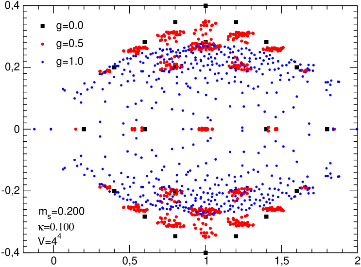
Figure 1: Spectrum of Wilson-Dirac operator for a small lattice and several values of the coupling.

Negative real part eigenvalues spoil the convergence of most iterative algorithms, but is not a fundamental problem. For larger values of the coupling and large lattices, nevertheless, the probability of having one -or more- eigenvalues very small grows dramatically. A simplified but significant picture can help to estimate the appearance of those small eigenvalues. The diagonal terms in (5) have the form $1+g_{L}\phi_{x}$, that will be zero as soon as $\phi_{x}=-1/g_{L}$. The values of $\phi_{x}$ are distributed according to (4), as a gaussian of width

$$\sigma^{2}=\sum_{k\in V}\frac{1}{\hat{k}^{2}+m_{s}^{2}}\ ,\qquad\hat{k}^{2}=2\sum_{\mu}(1-\cos(k_{\mu})).$$ (7)

The probability of having one negative eigenvalue is plotted in figure 2 for different lattice sizes, showing how negative eigenvalues appear for $g_{L}\sim 0.5$. The non diagonal terms in (5) modify this picture, and in practice there are small eigenvalues for $g_{L}\gtrsim 0.8$, hindering the numerical solution of the linear system. This implies that there is a maximum value of the coupling constant that can be used in this model. The problem could perhaps be solved in the unquenched case, as the fermionic determinant would eliminate the configurations with very small $\det(D)$.

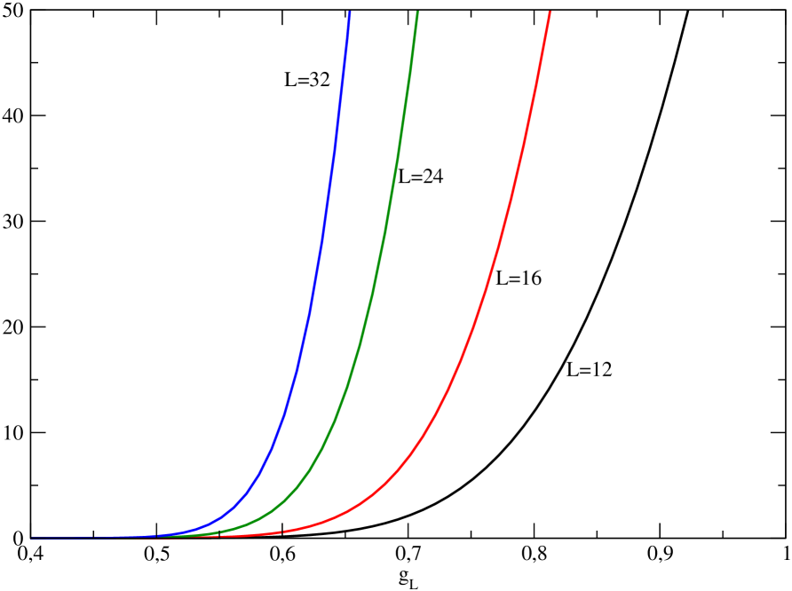
Figure 2: Average number of negative eigenvalues for several lattices with $Lam_{s}=5$ as a function of $g_{L}$.

4 One and two-body masses

One-body mass is computed from the time dependence of euclidean correlators:

$$C_{1}(t)=\sum_{\vec{x}}Tr\left[G(\vec{x},t)\right]\sim e^{-M_{1}t}\ ,$$ (8)

for large values of $t$, determining the fermion renormalized mass, $M_{1}$. Preliminary results on one body masses for both scalar and pseudoscalar coupling were already presented in qcd05 .

Two body masses, $M_{2}$, are obtained in a similar way, from the time evolution of the propagator of an operator $J(x)=\Gamma_{\alpha\beta}\psi_{\alpha}(x)\psi_{\beta}(x)$ creating a nucleon pair,

$$C_{2}(t)=\sum_{\bf x}Tr\langle J({\bf x},t)J^{\dagger}({\bf 0},0)\rangle\sim e^{-M_{2}t}\ ,$$

that for large values of $t$ projects on the lowest energy state with the quantum numbers of the operator $J(x)$. The matrix $\Gamma$ determines the spin and parity of the state, being $\Gamma=i\gamma_{2}\gamma_{0}\gamma_{5}$ for $J^{\pi}=0^{+}$ (ground state) and $\Gamma=\gamma_{2}\gamma_{0}$ for $J^{\pi}=0^{-}$.

The exponential behavior is reached only at large values of $t$. It is useful to define an effective mass as:

$$M_{eff}(t)=\ln\left(\frac{C(t)}{C(t+1)}\right)$$

that tends for large $t$ to the mass of the state and helps to find the adequate fitting window. Some results can be found in figure 3 for one and two body masses.

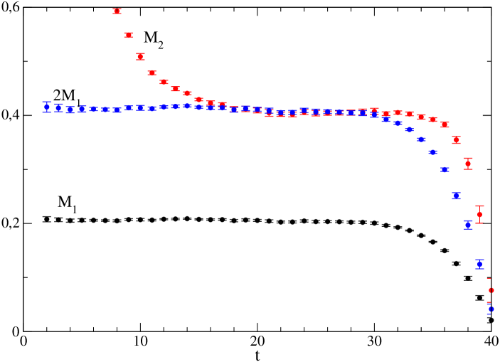
Figure 3: One and two body effective masses as a function of the euclidean time, for a $20^{3}\times 80$ lattice with $g_{0}\approx 1.6$ and $am_{s}=0.200$. In blue two times fermion mass, to compare with mass of two fermion $0^{+}$ state.

In the figure twice fermion mass is plotted for comparison. With these parameters twice fermion mass is not distinguishable of two fermion mass. This is the common picture for the whole set of parameters tested, no signal of the existence of a bound state is found below the critical value of the coupling constant .

5 Discussion

Renormalization effects have been analised for one body masses, where perturbation theory works, and the renormalization issues concerning the coupling constant have also been discussed qcd05 .

The existence of a maximum value of the coupling in a QFT treatment of the Yukawa model has been established. This critical value is smaller than the one needed to form a bound state in the NR limit, and no signal of such a bound state for lower couplings has been observed. This limit on the coupling is characteristic of the QFT, different from the potential approach where the coupling usually take values $G\gg 1$.

The meaning of this result needs to be clarified. It may be related to the quenched approximation, or the fact that we neglect meson self interaction. But then it should be noted that the same approximations are performed in the non relativistic (Schrodinger) treatment. For a given value of the lattice spacing, there exists other ways to discretize the nucleon-meson interaction which don’t have these zero modes. This has to be further studied and it is not clear if it allows to reach larger renormalized coupling constants and particularly to reach the bound regime. We are not yet in a position to decide if the bound on the coupling constant we encounter is a lattice artefact or if it really casts a doubt on the Yukawa theory itself.

It is known that the Yukawa theory is infrared free and, as such, encounters the “triviality problem” i.e. that the ultraviolet cut-off can not be driven to infinity without the theory becoming trivial. It means that this can only be an effective theory with a physical ultraviolet cut-off. The problem encountered from the difficulty to invert the Dirac operator seems also to put a limitation on the continuum limit. It is not clear whether both problems are related or just happen both to hinder the continuum limit.

Whether we manage or not to overcome the difficulty of reaching the domain where bound states appear, the connection between the QFT treatment and the Schrodinger approach can still be performed by an estimate of the scattering parameters which can be computed thanks to the method proposed by Luscher Luscher , and have recently been reexamined in ours ; fb18 .

References

- (1) V.G. Stoks et al. Phys. Rev. C49 (1994) 2950, R.B. Wiringa et al. Phys. Rev. C51 (1995) 38, R. Machleidt, Phys. Rev. C63 (2001) 0240041.
- (2) S.C. Pieper et al. Phys.Rev. C66 (2002) 044310
- (3) S. Weinberg, Nucl. Phys. B363 (1991) 3, C. Ordonez et al, Phys. Rev. C53 (1996) 2086, E. Epelbaum, W. Gockle, U.G. Meissner, Nucl. Phys. A671 (2000) 295.
- (4) T. Nieuwenhuis, J.A. Tjon, Phys. Rev. Let. 77 (1996), 814.
- (5) G. Baym, Phys. Rev 117 (1960), 886.
- (6) F. De Soto et al. hep-lat/0511009
- (7) M. Luscher, Commun. Math. Phys. 104 (1986) 177, Commun. Math. Phys. 105 (1986) 153, Nucl. Phys. B354 (1991), M. Luscher, Nucl. Phys. B364 (1991) 237.
- (8) F. De Soto and J. Carbonell, hep-lat/0610040
- (9) F. De Soto et al. hep-lat/0610086