Simulating at Realistic Quark Masses: Pseudoscalar Decay Constants and Chiral Logarithms

Abstract:

Due to improvements in computer performance and algorithms, the rapidly increasing cost for unquenched Wilson-type fermions with lighter quarks has been ameliorated and new simulations are now possible. Here we present results using two flavours of $O(a)$-improved Wilson fermions for meson decay constants at pseudoscalar masses down to 320 MeV. Results are at several lattice spacings down to about 0.07 fm and include a non-perturbative determination of the renormalisation constant. This enables us to attempt contact with (partially quenched) chiral perturbation theory.

1 Introduction

Chiral extrapolations of lattice data to the physical pion mass and the continuum or $a\to 0$ limit remain major sources of systematic uncertainty in the determination of hadron masses and matrix elements. A test that lattice QCD must successfully pass before predictions can be fully trusted is to reproduce known experimental results. One such indicator is the determination of meson decay constants, such as $f_{\pi^{+}}$ and $f_{K^{+}}$, with phenomenological values of $92.42\pm 0.07\pm 0.25\,\mbox{MeV}$ and $113.0\pm 1.0\pm 0.3\,\mbox{MeV}$, [1] respectively. The problem is that simulations for smaller quark masses rapidly become very costly in computer time. Recent advances have been on two fronts: firstly faster machines have become available, with speeds in the Tflop range and secondly the hybrid Monte Carlo algorithm used in the simulations has been improved. In particular in the new simulations reported here, we have used trajectory length one with three time scales in the molecular dynamic step (one for the glue term [2] and now two [3] for the fermion term in the action) which allowed the computationally expensive pieces to be updated less frequently. This was coupled with the use of an auxiliary fermion mass, [4].

The results reported here use Wilson glue (plaquette) and two mass degenerate $O(a)$-improved Wilson quarks (so effectively we are simulating 2-flavour QCD). As emphasised by Lüscher [5], these ‘clover’ fermions are well understood: in particular the addition of certain irrelevant terms, both in the action and operators, and the non-perturbative determination of their coefficients allow discretisation errors to be reduced to $O(a^{2})$. For example adding the ‘clover’ term together with the appropriate coefficient $c_{sw}$ is sufficient to determine the $O(a)$-improved masses, such as the pseudoscalar mass $m_{ps}$ while to determine the decay constant, given by

$$\langle 0|{\cal A}_{4}|ps\rangle={f_{ps}\over\sqrt{2}}m_{ps}\,,$$ (1)

the axial current $\cal A_{\mu}$ must also be $O(a)$-improved, which can be achieved by setting

$${\cal A}_{\mu}=Z_{A}{\cal A}_{\mu}^{\mbox{\tiny$I\!M\!P$}}\,,\qquad{\cal A}_{\mu}^{\mbox{\tiny$I\!M\!P$}}=\left(1+\mbox{\small$\frac{1}{2}$}b_{A}(am_{q_{1}}+am_{q_{2}})\right)\left(A_{\mu}+c_{A}a\partial_{\mu}P\right)\,,$$ (2)

where $A_{\mu}=\overline{q}_{1}\gamma_{\mu}\gamma_{5}q_{2}$ and $P=\overline{q}_{1}\gamma_{5}q_{2}$.

Several years ago we started simulations at four $\beta$ values and reached pseudoscalar masses of $\sim 600\,\mbox{MeV}$. We have started new simulations at $\beta=5.29$ and $\beta=5.40$ at lower quark masses. Our present status of the lower quark mass runs used in this report is given in table 1.

$\beta$	$\kappa^{S}$	Volume	Trajs	$m^{SS}_{ps}/m^{SS}_{vec}$	$m^{SS}_{ps}L$	$a[\mbox{fm}]$	$L[\mbox{fm}]$	$m^{SS}_{ps}[\mbox{MeV}]$
5.25	0.13575	$24^{3}\times 48$	6000	0.60	6.1	0.085	2.05	590
5.29	0.1359	$24^{3}\times 48$	4900	0.61	5.8	0.081	1.95	580
5.29	0.1362	$24^{3}\times 48$	3400	0.42	3.7	0.081	1.95	380
5.29	0.13632	$32^{3}\times 64$	1200	0.42	4.2	0.081	2.60	320
5.40	0.1361	$24^{3}\times 48$	3600	0.63	5.3	0.072	1.73	610
5.40	0.1364	$24^{3}\times 48$	2800	0.51	3.6	0.072	1.73	410

Table 1: Present data sets. The new runs are at $(\beta,\kappa^{S})=$ $(5.29,0.1362)$, $(5.29,0.13632)$ and $(5.40,0.1364)$, where ‘$S$’ means sea quark. $m^{SS}_{ps}$, $m^{SS}_{vec}$ are the pseudoscalar and vector particle masses respectively. $L$ is the box size. For comparison, experimentally $m_{\pi^{+}}/m_{\rho^{+}}\sim 0.18$ and $m_{\pi^{+}}\sim 140\,\mbox{MeV}$.

This has enabled us to reach pseudoscalar masses of $350\,\mbox{MeV}$ or less. The force-scale was the unit used to set the scale, together with a reference value $r_{0}=0.5\,\mbox{fm}$. Our results for $r^{S}_{0}/a$ are shown in fig. 1. In our extrapolations

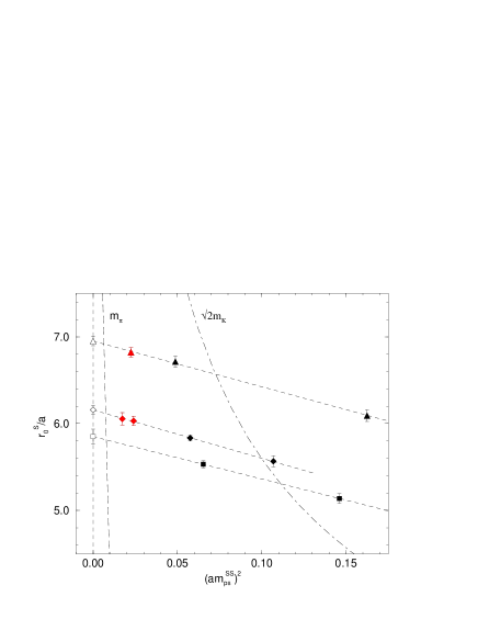
Figure 1: Results for $r_{0}^{S}/a$ versus $(am_{ps}^{SS})^{2}$ for $\beta=5.25$ (squares), $5.29$ (diamonds) and $5.40$ (triangles). The new runs are shown in red. Linear fits have been used to extrapolate $r^{S}_{0}/a$ to the chiral limit, the results being denoted by open symbols. The vertical dashed lines (left to right) represent the chiral limit, and using LO $\chi$PT approximate positions of a $\bar{l}l$, and fictitious $\bar{s}s$ pseudoscalar particle computed from $\pi^{+}$ and $K^{+}$ respectively.

we presently include results for heavier pseudoscalar masses; hopefully the situation will improve with more smaller quark mass results being generated so that a linear fit for the lighter quark masses will suffice. The extrapolated values of $r^{S}_{0}/a$ in the chiral limit $(r_{0}/a)_{c}$ are used to determine the scale.

2 Chiral perturbation theory

While the sea quark masses ($S$) are given (implicitly) in table 1, valence quarks ($V$) do not have to be chosen to have the same mass. Chiral Perturbation Theory, $\chi PT$, has been extended to Partially Quenched Chiral Perturbation Theory, $PQ\chi PT$, [6, 7]. While it is expensive to generate dynamical configurations, it is computationally cheaper to evaluate correlation functions on these configurations, so that a range of valence quark masses can be used. Using the Leading Order, LO, and Next to Leading Order, NLO, results [7] for the pseudoscalar masses and decay constants in terms of the quark mass, we eliminate (iteratively) the quark mass from these equations to give for degenerate mass valence quarks

$$F_{ps}^{VV}=f_{a}+f_{b}(M_{ps}^{SS})^{2}+f_{c}(M_{ps}^{VV})^{2}+f_{d}\left((M_{ps}^{SS})^{2}+(M_{ps}^{VV})^{2}\right)\ln\left((M_{ps}^{SS})^{2}+(M_{ps}^{VV})^{2}\right)\,,$$ (3)

where we have also rescaled the pseudoscalar mass, $m_{ps}^{AB}$, and decay constant, $f_{ps}^{AB}$ with say $r_{0c}$, ie

$$M_{ps}^{AB}=r_{0c}m_{ps}^{AB}\,,\qquad F_{ps}^{AB}=r_{0c}f_{ps}^{AB}\,,\qquad$$ (4)

with $A,B\in\{V,S\}$. $f_{a}$ (the LO result) and $f_{i}$, $i=b,c,d$ are given in terms of the low energy constants, LECs, $\alpha_{4}\sim-0.76$, $\alpha_{5}\sim 0.5$ (evaluated at a scale $\mu=\Lambda_{\chi}=4\pi f_{0}$) and $f_{0}\sim 86.2\,\mbox{MeV}$ (the decay constant in the chiral limit) [8] by

$$f_{a} = r_{0c}f_{0}$$

$$f_{b} = {1\over(4\pi)^{2}r_{0c}f_{0}}\left[{1\over 2}n_{f}\alpha_{4}+{1\over 4}n_{f}\ln\left(2(4\pi r_{0c}f_{0})^{2}\right)\right]$$

$$f_{c} = {1\over(4\pi)^{2}r_{0c}f_{0}}\left[{1\over 2}\alpha_{5}+{1\over 4}n_{f}\ln\left(2(4\pi r_{0c}f_{0})^{2}\right)\right]$$

$$f_{d} = -{1\over(4\pi)^{2}r_{0c}f_{0}}{1\over 4}n_{f}\,.$$ (5)

When $V=S$, eq. (3) further simplifies to

$$F_{ps}^{SS}=f_{a}+(f_{b}+f_{c}+2f_{d}\ln 2)(M_{ps}^{SS})^{2}+2f_{d}(M_{ps}^{SS})^{2}\ln(M_{ps}^{SS})^{2}\,.$$ (6)

From eq. (3) the pion and kaon decay constants can be found. We have two mass degenerate sea quarks which we associate with the light quark ($l$ where $m_{l}=(m_{u}+m_{d})/2$), together with two valence quarks, which we associate with either the light, $l$, quark or the strange, $s$, quark. Again manipulating the structural form of the LO and NLO equations gives the result

$$F_{\pi^{+}} = f_{a}+(f_{b}+f_{c}+2f_{d}\ln 2)M_{\pi^{+}}^{2}+2f_{d}M_{\pi^{+}}^{2}\ln M_{\pi^{+}}^{2}$$ (7)

$$F_{K^{+}} = f_{a}+\left(f_{b}+f_{d}\left(\ln 2+{2\over n_{f}^{2}}\right)\right)M_{\pi^{+}}^{2}+\left(f_{c}+f_{d}\left(\ln 2-{2\over n_{f}^{2}}\right)\right)M_{K^{+}}^{2}$$ (8)

$$+f_{d}\left(1-{1\over n_{f}^{2}}\right)M_{\pi^{+}}^{2}\ln M_{\pi^{+}}^{2}+{f_{d}\over n_{f}^{2}}M_{\pi^{+}}^{2}\ln\left(2M_{K^{+}}^{2}-M_{\pi^{+}}^{2}\right)+f_{d}M_{K^{+}}^{2}\ln M_{K^{+}}^{2}\,.$$

Determining the $f_{a}$ and $f_{i}$, $i=b,c,d$ coefficients means that the pion and kaon decay constants can be found. While degenerate quark masses are sufficient, see eq. (3), for both pion and kaon decay constants, only the pion decay constant is possible with just sea quarks, eq. (6).

Detecting chiral logarithms is a notorious problem, but is necessary as it shows that we are entering a regime where $\chi$PT is valid. This is particularly difficult for decay constants, as can be seen from eq. (3) that this term is $\propto\left((M_{ps}^{SS})^{2}+(M_{ps}^{VV})^{2}\right)\ln\left((M_{ps}^{SS})^{2}+(M_{ps}^{VV})^{2}\right)$ which for fixed $(M_{ps}^{SS})^{2}$ does not vary much with $(M_{ps}^{VV})^{2}$. We wish for a term $\propto(M_{ps}^{SS})^{2}\ln(M_{ps}^{VV})^{2}$. As suggested in [7] considering the ratio

$$R\equiv{F^{VS}_{ps}\over\sqrt{F^{VV}_{ps}F^{SS}_{ps}}}-1={f_{d}\over n_{f}^{2}f_{a}}\left((M_{ps}^{SS})^{2}\ln{(M_{ps}^{VV})^{2}\over(M_{ps}^{SS})^{2}}+(M_{ps}^{SS})^{2}-(M_{ps}^{VV})^{2}\right)\,,$$ (9)

(with $f_{d}/(n_{f}^{2}f_{a})=-1/(4n_{f}(4\pi r_{0c}f_{0})^{2})$ enhances these chiral logarithms. The disadvantage is that mixed quark mass correlators ($V\not=S$) must be computed. Note also that eqs. (3), (9) probe different parts of the $\chi$PT expression; as can be seen from eqs. (19) and (20) of [7], eq. (9) sees only the $O(1/n_{f})$ terms, while eq. (3) probes the remaining $O(1)$, $O(n_{f})$ terms.

3 Results

We use the well-established procedure outlined in [9] to compute decay constants. We only note here that in eq. (2), the improvement coefficient, $c_{A}$, has been computed non-perturbatively, [10], while $b_{A}$ is only known perturbatively (we use a tadpole improved version here, [11]). We expect, however, that as the quark masses used here are quite small this leads to negligible corrections. The renormalisation constant has also been non-perturbatively computed, [10, 11] (the differences between these results appear to be $O(a^{2})$ and hence vanish in the continuum limit).

We first investigate to see if we are entering a region where chiral logarithms are becoming visible. In fig. 2 we show $R$

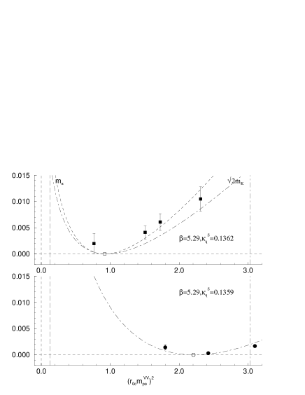
Figure 2: Results for $R$, eq. (9) for $(\beta,\kappa^{S})=(5.29,0.1359)$ (circles) and $(5.29,0.1362)$ (squares), against $(M_{ps}^{VV})^{2}\equiv(r_{0c}m^{VV}_{ps})^{2}$. The opaque symbols represent the points where $V\equiv S$ when $R\equiv 0$ identically. The dash-dotted curves are also defined in eq. (9) and are plotted with $c=-0.01659$ (using $r_{0}f_{0}\sim 0.218$). The dashed curve is a fit, yielding $c\sim-0.0227$ or $r_{0c}f_{0}\sim 0.187$. Other notation as fig. 1.

defined in eq. (9) for $\beta=5.29$ and $\kappa=0.1359$ and $0.1362$, together with the curve also given in eq. (9). While we do not expect much influence from the chiral logarithm, the curves track the data quite well, indeed out to reasonably large quark masses. So it would appear the chiral logarithms are visible of about the expected size. (But note the $y$-axis scale – we have subtracted $1$, so really this is a very small effect of $O(1\%)$.)

To determine the decay constants we must first take the continuum limit of the data, and then determine $f_{a}$ and $f_{i}$, $i=b,c,d$. But as $\chi$PT is an infra-red expansion, while the $a^{2}\to 0$ limit is ultra-violet and as we are using $O(a)$-improved fermions then we expect that there will be no problems with the order of the limits, ie first chiral and then continuum. More drastically we shall presently assume that we can ignore any $O(a^{2})$ error. This assumption must however be checked in the future.

We now turn to a consideration of the partially quenched results. In fig. 3

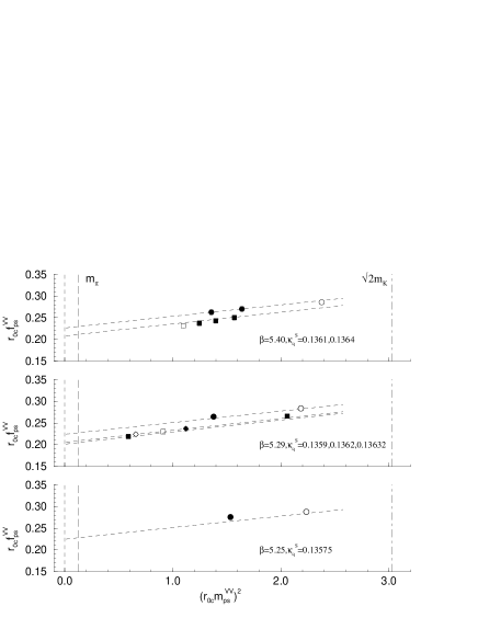
Figure 3: Results for $F_{ps}^{VV}\equiv r_{0c}f_{ps}^{VV}$ for the data sets given in table 1. The fit curves are given by eq. (3), for a common parameter set. The opaque symbols represent the points where $V\equiv S$. Other notation as fig. 1.

we show the results together with a fit from eq. (3). This is a global fit giving one parameter set $f_{a}$ and $f_{i}$, $i=b,c,d$ with values $0.190(16)$, $0.017(13)$, $0.030(12)$, $-0.0015(59)$ respectively. (The fit is reasonably good given the fact that the data has three varying parameters: $\beta$, $\kappa^{S}$ and $\kappa^{V}$.) We first note the the value of $f_{a}\equiv r_{0c}f_{0}$ is in good agreement with the value determined from $R$. However using this value to determine $f_{d}$ (see eq. (5)) gives $\sim-0.017$, indicating that we should be seeing a much stronger logarithmic dependence (indeed the curves are almost linear). Furthermore using $f_{a}$ and $f_{b}$, $f_{c}$ gives from eq. (5) the values $\alpha_{4}\sim-0.71$, $\alpha_{5}\sim-0.63$. $\alpha_{4}$ is in reasonable agreement with other phenomenological estimates; but $\alpha_{5}$ is not. So at the moment there is no unambiguous confirmation of $\chi$PT.

Consider now the sea quarks alone. In fig. 4

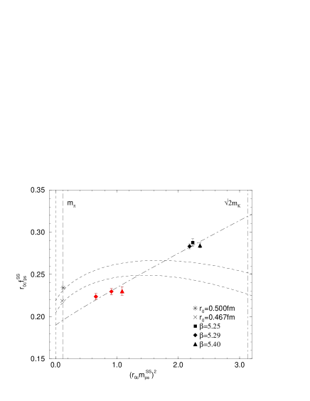
Figure 4: Results for $F_{ps}^{SS}\equiv r_{0c}m_{ps}^{SS}$ for the data sets in table 1. The fit curve (dashed-dotted line) is taken from eq. (6) using the parameters that have been determined from fig. 3. The dashed curves are possible phenomenological curves, using eqs. (5) and (6). The experimental value of $F_{\pi^{+}}\equiv r_{0}f_{\pi^{+}}$ is indicated by a star and cross for $r_{0}=0.5\,\mbox{fm}$ and $0.467\,\mbox{fm}$ respectively. Other notation as fig. 1.

we show these results. The curve joining the points uses the previously determined $f_{a}$, $f_{i}$, $i=b,c,d$ coefficients. Consistency is seen. The position of the new results is perhaps surprising because they have dropped to almost below where the phenomenological value might lie. Also shown is a possible phenomenological curve from eq. (5) for $r_{0}=0.5\,\mbox{fm}$. As previously found here there is little agreement with the lattice results. Reducing the $r_{0}$ scale helps somewhat, the second curve shows the phenomenological results using $r_{0}=0.467\,\mbox{fm}$, a result we estimated previously, see eg [11]. (This, of course, has the effect of making our pseudoscalar masses larger and box size smaller in table 1.) It would seem that the strict applicability of $\chi$PT is restricted to a rather narrow region $r_{0c}m^{SS}_{ps}\mathrel{\hbox to0.0pt{\lower 4.0pt\hbox{\hskip 1.0pt$\sim$}\hss}\raise 1.0pt\hbox{$<$}}1$; the choice of the scale is also rather delicate. Another issue are possible finite-size effects, which we are planning to investigate later.

Finally we note values of $f_{\pi^{+}}=77(4)\,\mbox{MeV}$, $f_{K^{+}}=93(1)\,\mbox{MeV}$ for $r_{0}=0.5\,\mbox{fm}$ and $f_{\pi^{+}}=82(5)\,\mbox{MeV}$, $f_{K^{+}}=98(2)\,\mbox{MeV}$ for $r_{0}=0.467\,\mbox{fm}$. Clearly using $f_{K^{+}}$ to set the scale would, at present, make the lattice finer. The dimensionless ratio $f_{K^{+}}/f_{\pi^{+}}$ is $\sim 1.21$, $1.19$ for $r_{0}=0.5\,\mbox{fm}$, $0.467\,\mbox{fm}$ respectively, to be compared with $(f_{K^{+}}/f_{\pi^{+}})_{expt}\sim 1.223$.

References

- [1] W.-M. Yao et al., J. Phys. G33 1 (2006).
- [2] A. Ali Khan et al., Phys. Lett. B564 235 (2003) [hep-lat/0303026].
- [3] C. Urbach et al., Comput. Phys. Commun. 174 87 (2006) [hep-lat/0506011].
- [4] M. Hasenbusch, Phys. Lett. B519 177 (2001) [hep-lat/0107019].
- [5] M. Lüscher, PoS LAT2005 002 (2005) [hep-lat/0509152].
- [6] C. Bernard et al., Phys. Rev. D49 486 (1994) [hep-lat/9306005].
- [7] S. R. Sharpe, Phys. Rev. D56 7052 (1997), erratum ibid. D62 099901 (2000) [hep-lat/9707018].
- [8] G. Colangelo et al., Eur. Phys. J. C33 543 (2004) [hep-lat/0311023].
- [9] M. Göckeler et al., Phys. Rev. D57 5562 (1998) [hep-lat/9707021].
- [10] M. Della Morte et al., JHEP 0503 029 (2005) [hep-lat/0503003].
- [11] A. Ali Khan et al., hep-lat/0603028.
- [12] M. Della Morte et al., JHEP 0507 007 (2005) [hep-lat/0505026].
- [13] C. R. Allton et al., Phys. Rev. D65 054502 (2002) [hep-lat/0107021].