Accelerating Staggered Fermion Dynamics with the
Rational Hybrid Monte Carlo (RHMC) Algorithm

Abstract

Improved staggered fermion formulations are a popular choice for lattice QCD calculations. Historically, the algorithm used for such calculations has been the inexact R algorithm, which has systematic errors that only vanish as the square of the integration step-size. We describe how the exact Rational Hybrid Monte Carlo (RHMC) algorithm may be used in this context, and show that for parameters corresponding to current state-of-the-art computations it leads to a factor of approximately seven decrease in cost as well as having no step-size errors.

Staggered fermions are a popular choice for lattice QCD calculations: they are generally thought of as being much cheaper than other fermion formulations, and have a remnant of the continuum theory’s chiral symmetry protecting them from additive mass renormalization. In order to overcome the infamous fermion doubling problem, the spin degrees of freedom are spatially separated reducing the $2^{4}$ fermion “tastes” to four. To further reduce these four tastes to a single quark (or doublet) the fourth (square) root of this kernel is taken. While this is a valid prescription in the continuum limit, it is unclear what unwanted side-effects this introduces to the lattice theory. At best this treatment is an algorithmic nuisance, at worst it renders the theory non-local, non-universal, and non-unitary rendering any calculations made using such a formulation questionable.

The reduction from 16 to 4 fermions also introduces $O(a^{2})$ unphysical taste-mixing interactions, where $a$ is the lattice spacing. There are various improved formulations of staggered fermions, all of which redefine the Dirac operator by some local averaging of the gauge field variables; the paths and coefficients of this averaging are chosen to minimize these unphysical interactions. The most popular formulation is the ASQTAD prescription, where the Dirac operator is constructed from a gauge covariant derivative consisting of the sum of the product of 1, 3, 5 and 7 link variables Orginos:1999cr .

After integrating out the Grassman-valued quark fields, the 2+1 quark flavor QCD partition function is given by a functional integral over gauge fields,

$$Z=\int dU\mathop{\rm det}({\cal M}_{\mbox{\tiny$\ell$}})^{\mathchoice{\textstyle{1\over 2}}{\scriptstyle{1\over 2}}{\scriptscriptstyle{1\over 2}}{1/2}}\mathop{\rm det}({\cal M}_{\mbox{\tiny s}})^{\mathchoice{\textstyle{1\over 4}}{\scriptstyle{1\over 4}}{\scriptscriptstyle{1\over 4}}{1/4}}e^{-S_{\mbox{\tiny G}}},\vspace{-2mm}$$

where $S_{\mbox{\tiny G}}$ is the gauge action (for ASQTAD fermions this is usually the one-loop improved Symanzik action) and ${\cal M}=-{\mathchoice{\mbox{D}\kern-6.49994pt\raise 0.6458pt\hbox{/}\kern 1.49994pt}{\mbox{D}\kern-6.49994pt\raise 0.6458pt\hbox{/}\kern 1.49994pt}{\mbox{\scriptsize D}\kern-5.0pt\raise 0.6458pt\hbox{\scriptsize/}}{\mbox{\tiny D}\kern-4.19998pt\raise 0.6458pt\hbox{\tiny/}}}^{2}+4m^{2}$ is the fermion matrix, with D/ being the staggered covariant derivative and $m$ the quark mass. The determinants represent the ($\ell$)ight and (s)trange quark contributions to the vacuum. It is the matrix square root and fourth root that make the formulation so algorithmically problematic: the Hybrid Monte Carlo (HMC) Duane:1987de algorithm commonly used for lattice calculations with dynamical fermions not being directly applicable.

The algorithm commonly used for performing these calculations is the Hybrid R algorithm Gottlieb:1987mq . First the identity $\mathop{\rm det}{\cal M}=\exp\mathop{\rm tr}\mathop{\rm ln}{\cal M}$ is used to write the action as

$$S=S_{\mbox{\tiny G}}-{\mathchoice{\textstyle{1\over 2}}{\scriptstyle{1\over 2}}{\scriptscriptstyle{1\over 2}}{1/2}}\mathop{\rm tr}\mathop{\rm ln}{\cal M}_{\mbox{\tiny$\ell$}}-{\mathchoice{\textstyle{1\over 4}}{\scriptstyle{1\over 4}}{\scriptscriptstyle{1\over 4}}{1/4}}\mathop{\rm tr}\mathop{\rm ln}{\cal M}_{\mbox{\tiny s}},\vspace{-2mm}$$

then a Gaussian-distributed “fictitious” momentum field $\pi$, taking values in the Lie algebra $su(3)$ on links, is introduced so a Hamiltonian $H={\mathchoice{\textstyle{1\over 2}}{\scriptstyle{1\over 2}}{\scriptscriptstyle{1\over 2}}{1/2}}\pi^{2}+S$ may be defined. Configurations $(\pi,U)$ are then generated with probability proportional to $e^{-H}$ by alternating two Markov steps, refreshment of the momenta from a Gaussian heatbath and evolution of the gauge fields following the MD (MD) trajectory defined by this Hamiltonian for time $\tau$. The MD trajectory is approximated by means of a numerical integrator with a step-size of $\delta\tau$, so these steps give an ergodic Markov process with the desired fixed point up to step-size errors. Usually the second order leapfrog (2LF) integrator is used which requires a single force evaluation per step, and this leads to errors of $O(\delta\tau^{2})$ in the coefficients in the action.

The fermionic contribution to the force acting on the gauge fields is approximated by means of a noisy estimator for each trace appearing in the action: this requires the introduction of an auxiliary “noise” field that is refreshed after every update. Each fermion force evaluation requires that the inverse fermion matrix be applied to its auxiliary field, typically by means of a conjugate gradient (CG) solver. The cost of the algorithm increases dramatically as the fermion mass is taken to zero, and the cost of the light quarks contribution dominates that of the strange.

Additional $O(\delta\tau)$ errors are introduced by using noisy estimates of the fermionic force, regardless of the numerical integrator used. These may be made to vanish by refreshing the auxiliary field at an asymmetric time within each update step, dependent on the number of fermions; doing so leads to an integrator that is neither area-preserving nor reversible, and therefore the step-size errors cannot be removed by means of a Metropolis acceptance test as with HMC. The R algorithm is thus necessarily an inexact algorithm with $O(\delta\tau^{2})$ errors.

An alternative approach is to represent each fermionic determinant as a Gaussian integral over a bosonic “pseudofermion” field $\phi$: the resulting fermion action is $S_{\mbox{\tiny F}}=\phi_{\mbox{\tiny$\ell$}}^{\dagger}{\cal M}_{\mbox{\tiny$\ell$}}^{-{\mathchoice{\textstyle{1\over 2}}{\scriptstyle{1\over 2}}{\scriptscriptstyle{1\over 2}}{1/2}}}\phi_{\mbox{\tiny$\ell$}}+\phi_{\mbox{\tiny s}}^{\dagger}{\cal M}_{\mbox{\tiny s}}^{-{\mathchoice{\textstyle{1\over 4}}{\scriptstyle{1\over 4}}{\scriptscriptstyle{1\over 4}}{1/4}}}\phi_{\mbox{\tiny s}}$. At this point the conventional HMC algorithm fails as one can neither evaluate the $n^{\mbox{\tiny th}}$ root of a matrix directly nor calculate its derivative with respect to the gauge field as required for the MD evolution of the system. However, it is possible to replace the matrix kernel with an approximation that can be evaluated and differentiated. There are two obvious approximations: polynomial deForcrand:1996ck ; Frezzotti:1997ym and rational Kennedy:1998cu ; Clark:2004cp . Polynomial approximations do not require the explicit evaluation of a matrix inverse, but they typically have to be of much higher degree than the corresponding rational approximations with the same error: for example, a polynomial approximation to $1/{\cal M}$ for an hermitian matrix ${\cal M}$ is equivalent to computing the inverse by means of a Jacobi iteration scheme, and this is well-known to be far inferior to other iterative solvers such as CG. With this in mind, we focus on optimal rational approximations (generally found using the Remez algorithm). We replace the square and fourth root kernels by rational approximations, and continue as if we would for HMC, for which each complete update consists of a sequence of the following Markov steps

• Momentum refreshment heatbath using Gaussian noise ($P(\pi)\propto e^{-\pi^{2}/2}$).

• Pseudofermion refreshment ($P(\phi)\propto{\cal M}^{\frac{1}{2\alpha}}\eta$, where $P(\eta)\propto e^{-\eta^{2}/2}$, $\alpha=2$(4) for light (strange)).

• MDMC update, built out of

  • A (MD) trajectory consisting of $\tau/\delta\tau$ steps.

  • A Metropolis accept/reject with probability $P_{\mbox{\tiny acc}}=\min(1,e^{-\delta H})$.

The key advantage over the R algorithm is that the Metropolis test at the end of the trajectory stochastically corrects any finite step-size errors introduced through the discretized MD integration.

It is necessary to generate the pseudofermion fields at the start of each trajectory from a heatbath. For the functions of interest, the roots and poles of optimal (in the minimax $=L_{\infty}=$ Chebyshev norm) rational approximations are real and non-degenerate: this motivates a fermionic action $S_{\mbox{\tiny F}}=\phi_{\mbox{\tiny$\ell$}}^{\dagger}[r_{\mbox{\tiny$\ell$}}^{\mbox{\tiny MC}}({\cal M}_{\mbox{\tiny$\ell$}})]^{2}\phi_{\mbox{\tiny$\ell$}}+\phi_{\mbox{\tiny s}}^{\dagger}[r_{\mbox{\tiny s}}^{\mbox{\tiny MC}}({\cal M}_{\mbox{\tiny s}})]^{2}\phi_{\mbox{\tiny s}}$, where $r_{\mbox{\tiny$\ell$}}^{\mbox{\tiny MC}}(x)\approx x^{-{\mathchoice{\textstyle{1\over 4}}{\scriptstyle{1\over 4}}{\scriptscriptstyle{1\over 4}}{1/4}}}$ and $r_{\mbox{\tiny s}}^{\mbox{\tiny MC}}(x)\approx x^{-{\mathchoice{\textstyle{1\over 8}}{\scriptstyle{1\over 8}}{\scriptscriptstyle{1\over 8}}{1/8}}}$ are valid over the spectral bounds of the operator. These rational approximations must in some sense be exact: typically this means the maximum error is either less than the tolerance used in the solver or, more conservatively, less than the unit of least precision of double precision arithmetic ($\approx 10^{-15}$).

When written in partial fraction form (we consider only the case where the numerator and denominator polynomial degrees are equal) $r(x)=\alpha_{0}+\sum_{k=1}^{n}\frac{\alpha_{k}}{x+\beta_{k}},$ where $n$ is the degree of the approximation. It transpires that for the cases of interest all the $\alpha_{k}$ and $\beta_{k}$ are real and positive: this ensures numerical stability of the method.

A multi-shift solver Frommer:1995ik can be used to evaluate the rational approximation with a cost similar to that of the inversion of the original matrix ${\cal M}$, thus both the pseudofermion heatbath and the evaluation of the action for the Metropolis step can be carried out within a single Krylov space. A difficulty arises when the fermionic force has to be computed, as this seems to depend upon the derivative of the square of the rational approximation $r$, which involves double poles; this is obviously undesirable, as naïvely it doubles the cost as compared to the R algorithm. However, there is no reason why the MD and MC approximations need be the same: one is free to choose the MD approximation to avoid the square, and also use a lower degree approximation should one so wish. Indeed, the optimal approximation to ${\cal M}^{2\alpha}$ is not the square of that for ${\cal M}^{\alpha}$ anyhow. The MD action is thus written

$$S_{\mbox{\tiny F}}^{\mbox{\tiny MD}}=\phi_{\mbox{\tiny$\ell$}}^{\dagger}r_{\mbox{\tiny$\ell$}}^{\mbox{\tiny MD}}({\cal M}_{\mbox{\tiny$\ell$}})\phi_{\mbox{\tiny$\ell$}}+\phi_{\mbox{\tiny s}}^{\dagger}r_{\mbox{\tiny s}}^{\mbox{\tiny MD}}({\cal M}_{\mbox{\tiny s}})\phi_{\mbox{\tiny s}},\vspace{-1mm}$$ (1)

where the approximations $r_{\mbox{\tiny$\ell$}}^{\mbox{\tiny MD}}(x)\approx x^{-{\mathchoice{\textstyle{1\over 2}}{\scriptstyle{1\over 2}}{\scriptscriptstyle{1\over 2}}{1/2}}}$ and $r_{\mbox{\tiny s}}^{\mbox{\tiny MD}}(x)\approx x^{-{\mathchoice{\textstyle{1\over 4}}{\scriptstyle{1\over 4}}{\scriptscriptstyle{1\over 4}}{1/4}}}$ are again valid over the appropriate spectral ranges.

The derivative of each of the bilinear terms that appear in equation (1) is written as

$$S_{\mbox{\tiny F}}^{\prime} = -\sum_{k=1}^{n}{X^{(k)}}^{\dagger}{\cal M}^{\prime}X^{(k)}$$ (2)

$$= -\mathop{\rm tr}\Bigl{[}{\cal M}^{\prime}\sum_{k=1}^{n}X^{(k)}\otimes{X^{(k)}}^{\dagger}\Bigr{]},\vspace{-2mm}$$ (3)

where $X_{k}=\sqrt{\alpha_{k}}({\cal M}+\beta_{k})^{-1}\phi$. The calculation of ${\cal M}^{\prime}$ must be done explicitly using the chain rule and represents a considerable computational expense because of the complicated nature of the ASQTAD operator. The only dependence on the pseudofermion fields is in $X^{(k)}$, and even if there are many such fields one need only calculate ${\cal M}^{\prime}$ once. For $n>3$ it is more expensive to use matrix-vector operations (2) than matrix-matrix operations (3), hence we use the latter Clark:2004cp .

The naïve cost of RHMC is similar to that of the R algorithm at the same step-size: however, the actual cost is determined by the integration step-size that can be used, and the algorithms’ respective autocorrelations.

Before we present results from such a comparison, we describe a reformulation of the fermion action which greatly reduces the cost of RHMC. It has been shown that “mass preconditioning” the fermion force leads to a large reduction in the computational cost Hasenbusch:2001ne ; the fermion kernel is multiplied by the inverse of a similar kernel with a larger mass, and the desired distribution is then recovered by also introducing a new pseudofermion field with this larger mass kernel. This is beneficial because the resulting pseudofermion kernels are less singular, and thus lead to smaller forces acting on the gauge fields; this in turn permits the use of a larger integration step-size before the symplectic integrator becomes unstable. A multiple timescale numerical integrator where the mass preconditioned light pseudofermion force is evaluated less often than that of the new pseudofermion then gives further speed-up: when tuning such an algorithm the product of each step-size with the magnitude of the corresponding force contribution should be the same to a first approximation.

In previous work Urbach:2005ji mass preconditioning was applied to $2$ flavor Wilson fermion calculations, but neither to $2+1$ quark flavors nor to staggered fermions, both of which lend themselves particularly well to this technique because the strange quark can be used as a preconditioner, as shall now be explained. The $2+1$ flavor staggered determinant may be written as

$$\mathop{\rm det}({\cal M}_{\mbox{\tiny$\ell$}})^{\mathchoice{\textstyle{1\over 2}}{\scriptstyle{1\over 2}}{\scriptscriptstyle{1\over 2}}{1/2}}\mathop{\rm det}({\cal M}_{\mbox{\tiny s}})^{\mathchoice{\textstyle{1\over 4}}{\scriptstyle{1\over 4}}{\scriptscriptstyle{1\over 4}}{1/4}}=\left(\frac{\mathop{\rm det}({\cal M}_{\mbox{\tiny$\ell$}})}{\mathop{\rm det}({\cal M}_{\mbox{\tiny s}})}\right)^{\mathchoice{\textstyle{1\over 2}}{\scriptstyle{1\over 2}}{\scriptscriptstyle{1\over 2}}{1/2}}\,\mathop{\rm det}({\cal M}_{\mbox{\tiny s}})^{\mathchoice{\textstyle{3\over 4}}{\scriptstyle{3\over 4}}{\scriptscriptstyle{3\over 4}}{3/4}},\vspace{-2mm}$$

where the light quark has been “mass preconditioned” by the strange quark. The corresponding action is

$$S_{\mbox{\tiny F}} = \phi_{\mbox{\tiny$\ell$}}^{\dagger}\left(\frac{{\cal M}_{\mbox{\tiny s}}}{{\cal M}_{\mbox{\tiny$\ell$}}}\right)^{\mathchoice{\textstyle{1\over 2}}{\scriptstyle{1\over 2}}{\scriptscriptstyle{1\over 2}}{1/2}}\phi_{\mbox{\tiny$\ell$}}+\phi_{\mbox{\tiny s}}^{\dagger}{\cal M}_{\mbox{\tiny s}}^{-{\mathchoice{\textstyle{3\over 4}}{\scriptstyle{3\over 4}}{\scriptscriptstyle{3\over 4}}{3/4}}}\phi_{\mbox{\tiny s}}$$ (4)

$$= \phi_{\mbox{\tiny$\ell$}}^{\dagger}\left(\frac{{\cal M}_{\mbox{\tiny$\ell$}}+\delta m^{2}}{{\cal M}_{\mbox{\tiny$\ell$}}}\right)^{\mathchoice{\textstyle{1\over 2}}{\scriptstyle{1\over 2}}{\scriptscriptstyle{1\over 2}}{1/2}}\phi_{\mbox{\tiny$\ell$}}+\phi_{\mbox{\tiny s}}^{\dagger}{\cal M}_{\mbox{\tiny s}}^{-{\mathchoice{\textstyle{3\over 4}}{\scriptstyle{3\over 4}}{\scriptscriptstyle{3\over 4}}{3/4}}}\phi_{\mbox{\tiny s}}$$

$$\approx \phi_{\mbox{\tiny$\ell$}}^{\dagger}r_{\mbox{\tiny$\ell$}}({\cal M}_{\mbox{\tiny$\ell$}})\phi_{\mbox{\tiny$\ell$}}+\phi_{\mbox{\tiny s}}^{\dagger}r_{\mbox{\tiny s}}({\cal M}_{\mbox{\tiny s}})\phi_{\mbox{\tiny s}},\vspace{-2mm}$$

where in the second line use has been made of the fact that the staggered quark mass is additive, ${\cal M}_{\mbox{\tiny s}}={\cal M}_{\mbox{\tiny$\ell$}}+\delta m^{2}$ with $\delta m^{2}\equiv 4(m_{\mbox{\tiny s}}^{2}-m_{\mbox{\tiny$\ell$}}^{2})$, so that the first term may be written in terms of a single rational function of the light quark kernel in equation (4). The cost of evaluating the action is almost unchanged since no extra fields have been introduced, rather better use is being made of the already present strange quark. Since the light quark is preconditioned by the strange quark we expect that its contribution to the total force will be small in comparison to the “triple strange”. This is advantageous because the triple strange force is much cheaper to evaluate since it is a rational approximation of the more massive strange quark kernel. Thus the hierarchy of the integrators is to have the gauge field force updates (which are cheap compared with fermionic force evaluations) on the smallest time scale, the triple strange on an intermediate scale, and the preconditioned light quark on the largest scale. We note that choosing the strange quark to precondition the light quarks is merely down to the former’s presence: if the strange quark were not already present then the optimal precondittioned would certainly have a difference mass. Figure 1 is an example of the effect the mass conditioning has on the forces: the vast reduction in magnitude of the light quark contribution is evident.

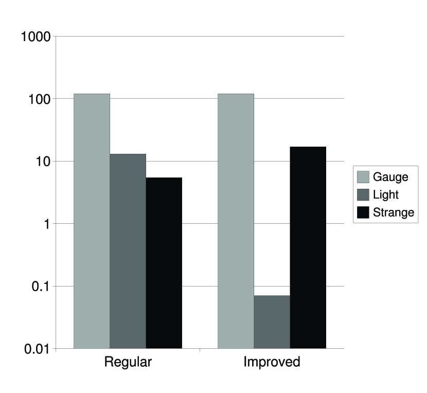
Figure 1: A comparison of the relative $L_{\infty}$ magnitude of the forces of the original $2+1$ RHMC ASQTAD formulation, and that of the mass preconditioned one. In the former the light quark force is more than three times that of the strange contribution, in the latter it is two orders of magnitude smaller ($V=4^{4}$, $\beta=6.76$, $m_{\mbox{\tiny$\ell$}}=0.01$, $m_{\mbox{\tiny s}}=0.05$).

A nice side effect of such mass preconditioning is that the approximation degree required for the preconditioned light kernel is much less than for the original one because its kernel is much better conditioned.

As well as mass preconditioning, there are other improvements that can be made to the RHMC algorithm. The $n^{\mbox{\tiny th}}$ root multiple pseudofermion trick Clark:2004cq can be used to allow a larger integration step-size at constant acceptance rate: here one pseudofermion with kernel ${\cal M}^{\alpha}$ is replaced by $n$ pseudofermions each with kernel ${\cal M}^{\alpha/n}$. This method removes the integrator instability, after which it becomes advantageous to use higher-order or improved integrators Clark:2006fx , e.g., a second order minimum norm (2MN) integrator Takaishi:2005tz . The tolerance of the MD solver can be tuned on a per-shift basis; in particular the tolerances of least well-conditioned shifts can be loosened considerably with little affect on the acceptance rate. This leads to a large reduction in the number of CG iterations Clark:2005sq .

In order to test the improved RHMC algorithm, a suitably challenging set of parameters were chosen, as specified in Table 1. These parameters also represent a recent run of the R algorithm performed by the MILC collaboration, so a direct comparison is possible.

	R MILC	RHMC
$\tau/\delta\tau$	$300$	$5_{\mbox{\tiny s,$\ell$}},25_{\mbox{\tiny gauge}}$
$(n_{\mbox{\tiny MD}},n_{\mbox{\tiny MC}})$	—	$(6,10)_{\mbox{\tiny s}}$, $(4,7)_{\mbox{\tiny$\ell$}}$
$\mathop{\rm res}_{\mbox{\tiny MD}}$	$(5\cdot 10^{-5})_{\mbox{\tiny s,$\ell$}}$	$(10^{-4})_{\mbox{\tiny s}}$, $(10^{-5})_{\mbox{\tiny$\ell$}}$
$\mathop{\rm res}_{\mbox{\tiny MC}}$	—	$(10^{-10})_{\mbox{\tiny s,$\ell$}}$
$N_{\mbox{\tiny cg}}$	344,988	70,230
$N_{\mbox{\tiny flops}}$	$5.96\times 10^{14}$	$8.54\times 10^{13}$
$\langle P_{\mbox{\tiny acc}}\rangle$	—	0.775(23)

Table 1: Parameters and performance: $n$ denotes the rational approximation degree, $P_{\mbox{\tiny acc}}$ the Metropolis acceptance rate, and $\mathop{\rm res}$ the CG solver residual. The subscripts s and $\ell$ indicate the fermion flavor. $N_{\mbox{\tiny cg}}$ and $N_{\mbox{\tiny flops}}$ are the total CG iterations and floating point operations per trajectory respectively. The computations were performed on a $V=24^{3}.64$ lattice with $\beta=6.76$, $m_{\mbox{\tiny$\ell$}}=0.005$, $m_{\mbox{\tiny s}}=0.05$, and $\tau=1.0$.

From previous studies of the R algorithm it has been found empirically that choosing an integrator step-size $\delta\tau\approx{\mathchoice{\textstyle{2\over 3}}{\scriptstyle{2\over 3}}{\scriptscriptstyle{2\over 3}}{2/3}}m_{\mbox{\tiny$\ell$}}$ leads to step-size errors that are deemed to be negligible. On the other hand, deciding on the optimum step-sizes for multiple timescale RHMC algorithm is a more involved process. When constructing the multi-scale integrator, it was decided to evaluate the gauge force using a fourth order integrator Takaishi:2005tz to minimize this part of the cost. After constructing the multiple timescale integrator, a single MD trajectory was used to measure the force contributions in order to estimate the step-size ratios. It was observed that the cost of the calculation was dominated by the triple strange; this in turn was dominated by the calculation of the matrix derivative, and not the matrix inversion (this effect is exacerbated by the tolerance loosening optimization); thus any further mass preconditioning would be of little benefit. To further reduce the algorithm cost, the $n^{\mbox{\tiny th}}$ root multiple pseudofermion formulation was used for the triple strange, with $3$ pseudofermions, this allowed for a large increase of step-size, so much so in fact that the optimal parameters were found to be those where the light and triple strange were all on the same time scale again, i.e., a two level integrator separating the fermion and gauge timescales. It is interesting to note that the optimal algorithm for 2+1 flavour ASQTAD fermions requires both mass preconditioning and the $n^{\mbox{\tiny th}}$ root trick, emphasizing the opinion expressed in Clark:2004cq that these approcahes can be complimentary.

A summary of the optimal parameters and costs is given in Table 1. Perhaps the most interesting result is the factor of 7 reduction in the number floating point operations per trajectory relative to the R algorithm. It must be emphasized this factor does not take into

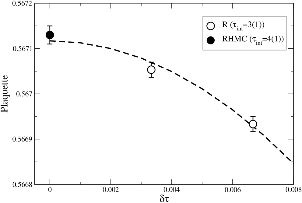
Figure 2: An extrapolation of the plaquette in $\delta\tau$ comparing the exact RHMC result with the inexact R result MILC .

account the additional benefit of using an exact algorithm over an inexact one, illustrated in figure 2. The autocorrelation lengths of the plaquette using the algorithms are similar, indeed they are essentially the same after dividing by RHMC’s acceptance rate, and this is expected to be true for all other autocorrelations too.

In this letter, we have described the exact RHMC algorithm, and how this algorithm can be used to greatly accelerate the generation of lattice QCD gauge field ensembles with dynamical ASQTAD fermions compared to current techniques using the inexact R algorithm. Through a switch of algorithm, a production job that takes a year becomes at worst a matter of months, while at the same time removing a source of systematic error.

References

- (1) Kostas Orginos, Doug Toussaint, and R. L. Sugar. Phys. Rev., D60, 054503, 1999 (hep-lat/9903032).
- (2) S. Duane, A. D. Kennedy, B. J. Pendleton, and D. Roweth. Phys. Lett., B195, 216–222, 1987.
- (3) Steven A. Gottlieb, W. Liu, D. Toussaint, R. L. Renken, and R. L. Sugar. Phys. Rev., D35, 2531–2542, 1987.
- (4) Philippe de Forcrand and Tetsuya Takaishi. Nucl. Phys. Proc. Suppl., bf 53, 968–970, 1997 (hep-lat/9608093).
- (5) Roberto Frezzotti and Karl Jansen. Phys. Lett., B402, 328–334, 1997 (hep-lat/9702016).
- (6) A. D. Kennedy, Ivan Horvath, and Stefan Sint. Nucl. Phys. Proc. Suppl., 73, 834–836, 1999 (hep-lat/9809092).
- (7) M. A. Clark, A. D. Kennedy, and Z. Sroczynski. Nucl. Phys. Proc Suppl., B140, 835, 2005 (hep-lat/0409133).
- (8) Andreas Frommer, Bertold Nockel, Stephan Gusken, Thomas Lippert, and Klaus Schilling. Int. J. Mod. Phys., C6, 627–638, 1995 (hep-lat/9504020).
- (9) Martin Hasenbusch. Phys. Lett., B519, 177–182, 2001 (hep-lat/0107019).
- (10) C. Urbach, K. Jansen, A. Shindler, and U. Wenger. Comput. Phys. Commun., 174 87–98, 2006 (hep-lat/0506011).
- (11) Tetsuya Takaishi and Philippe de Forcrand. Phys. Rev., E73 036706, 2006 (hep-lat/0505020).
- (12) M. A. Clark and A. D. Kennedy. Nucl. Phys. Proc. Suppl., B140, 838, 2005 (hep-lat/0409134).
- (13) M. A. Clark and A. D. Kennedy. 2006 (hep-lat/0608015).
- (14) M. A. Clark, Ph. de Forcrand, and A. D. Kennedy. PoS, LAT2005:115, 2005 (hep-lat/0510004).
- (15) MILC collaboration. Private communication.