Generalized Potts-Models and their Relevance for Gauge Theories

Generalized Potts-Models and their Relevance
for Gauge Theories

Andreas WIPF ^†, Thomas HEINZL ^‡, Tobias KAESTNER ^† and Christian WOZAR ^† A. Wipf, T. Heinzl, T. Kaestner and C. Wozar

^† Theoretisch-Physikalisches Institut, Friedrich-Schiller-University Jena, Germany

wipf@tpi.uni-jena.de http://www.personal.uni-jena.de/~p5anwi/ ^‡ School of Mathematics and Statistics, University of Plymouth, United Kingdom thomas.heinzl@plymouth.ac.uk

Received October 05, 2006, in final form December 12, 2006; Published online January 05, 2007

We study the Polyakov loop dynamics originating from finite-temperature Yang–Mills theory. The effective actions contain center-symmetric terms involving powers of the Polyakov loop, each with its own coupling. For a subclass with two couplings we perform a detailed analysis of the statistical mechanics involved. To this end we employ a modified mean field approximation and Monte Carlo simulations based on a novel cluster algorithm. We find excellent agreement of both approaches. The phase diagram exhibits both first and second order transitions between symmetric, ferromagnetic and antiferromagnetic phases with phase boundaries merging at three tricritical points. The critical exponents $\nu$ and $\gamma$ at the continuous transition between symmetric and antiferromagnetic phases are the same as for the 3-state spin Potts model.

gauge theories; Potts models; Polyakov loop dynamics; mean field approximation; Monte Carlo simulations

81T10; 81T25; 81T80

1 Introduction

Symmetry constraints and strong coupling expansion for the effective action describing the Polyakov loop dynamics of gauge theories lead to effective field theories with rich phase structures. The fields are the fundamental characters of the gauge group with the fundamental domain as target space. The center symmetry of pure gauge theory remains a symmetry of the effective models. If one further freezes the Polyakov loop to the center ${\cal Z}$ of the gauge group one obtains the well known vector Potts spin-models, sometimes called clock models. Hence we call the effective theories for the Polyakov loop dynamics generalized ${\cal Z}$-Potts models. We review our recent results on generalized $\mbox{\af Z}_{3}$-Potts models [2]. These results were obtained with the help of an improved mean field approximation and Monte Carlo simulations. The mean field approximation turns out to be much better than expected. Probably this is due to the existence of tricritical points in the effective theories. There exist four distinct phases and transitions of first and second order. The critical exponents $\nu$ and $\gamma$ at the second order transition from the symmetric to antiferromagnetic phase for the generalized Potts model are the same as for the corresponding Potts spin model.

Earlier on it had been conjectured that the effective Polyakov loop dynamics for finite temperature $SU(N)$ gauge theories near the phase transition point is very well modelled by $3$-dimensional $\mbox{\af Z}_{N}$ spin systems [3, 4]. For $SU(2)$ this conjecture is supported by universality arguments and numerical simulations. The status of the conjecture for $SU(3)$ gauge theories is unclear, since the phase transition is first order such that universality arguments apparently are not applicable.

2 Recall of planar Potts models

The $q$-state Potts model [5, 6, 7] is a natural extension of the Ising model. On every lattice site $x$ there is a planar vector with unit length which may point in $q$ different directions (Fig. 1) with angles

Figure 1: Angles in a $q$-state Potts model.

$$\theta_{x}\in\left\{\frac{2\pi}{q},\frac{4\pi}{q},\dots,2\pi\right\}=\mbox{\af Z}_{q}.$$

Only nearest neighbors interact and their contribution to the energy is proportional to the scalar product of the vectors, such that

$$H=-J\sum_{\langle xy\rangle}\cos\left(\theta_{x}-\theta_{y}\right).$$ (2.1)

The Hamiltonian $H$ is invariant under simultaneous rotations of all vectors by a multiple of $2\pi/q$. These $\mbox{\af Z}_{q}$ symmetries map a configuration $w=\{\theta_{x}|x\in\Lambda\}$ into $w^{\prime}=\{\theta_{x}+2\pi n/q\},\;n\in\{1,\dots,q\}$. In two and higher dimensions the spin model shows a phase transition at a critical coupling $K_{c}=\beta J_{c}>0$ from the symmetric to the ferromagnetic phase. In two dimensions this transition is second order for $q\leq 4$ and first order for $q>4$. In three dimensions it is second order for $q\leq 2$ and first order for $q>2$.

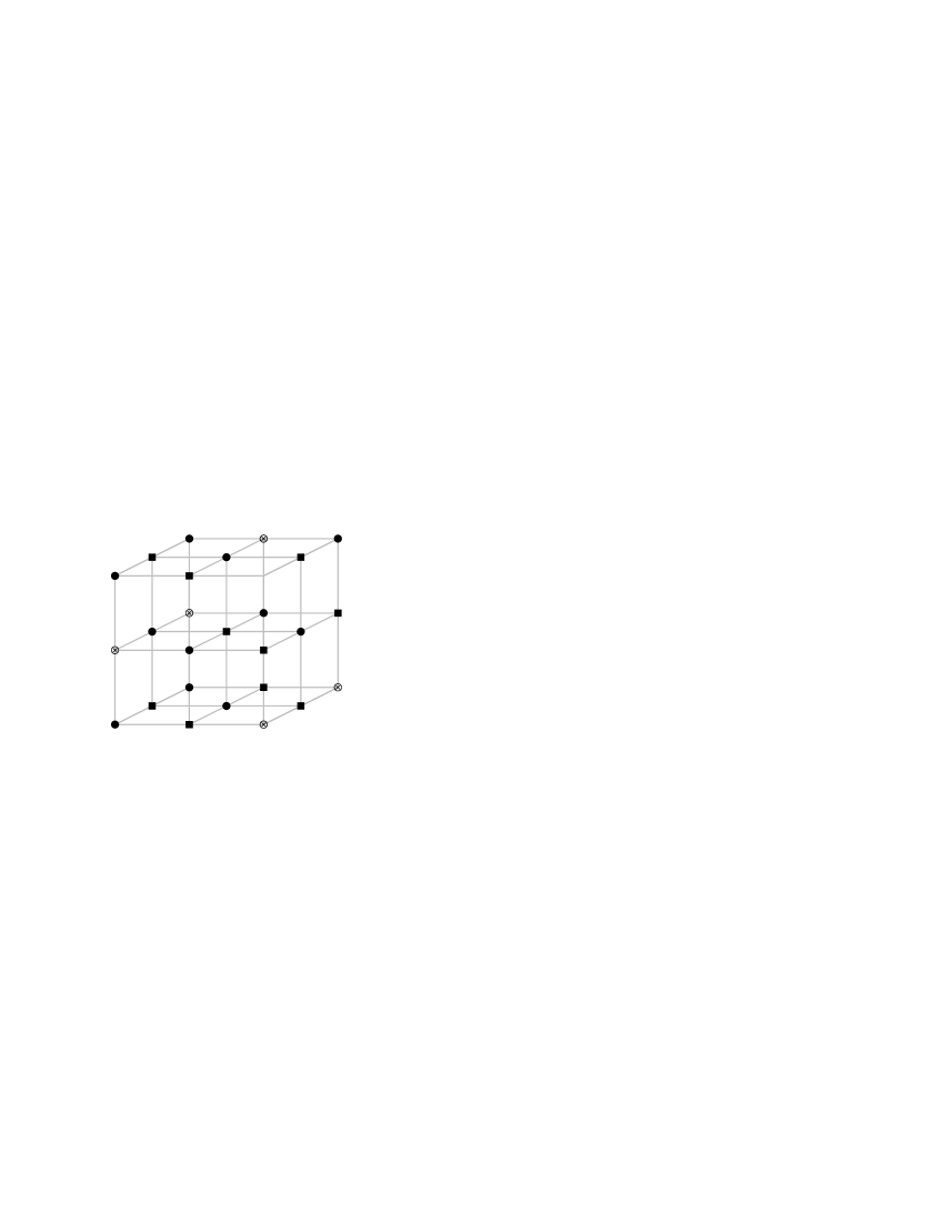
Figure 2: Coloring of neighboring lattice sites.

There is another phase transition at negative critical coupling $K^{\prime}_{c}$ from the symmetric to the antiferromagnetic phase. For $q\geq 3$ and negative $K$ the number of ground states of (2.1) increases rapidly with the number of lattice sites. It equals the number of ways one can color the vertices with $q$ colors such that two neighboring sites have different colors (Fig. 2). In the antiferromagnetic case the degenerate ground states contribute considerably to the entropy [8]

$$S_{B}(P)=-\sum P(w)\log P(w),$$

where one sums over all spin configurations and $P$ is the probability of $w$. We use the well known variational characterization of the free energy,

$$\beta F=\inf_{P}\left(\beta\langle H\rangle_{P}-S_{B}\right),\qquad\langle H\rangle_{P}=\sum_{w}P(w)H(w),$$

where the minimum is to be taken on the space of all probability measures. The unique minimizing probability measure is the Gibbs state

$$P_{\rm Gibbs}\sim e^{-\beta H}$$ (2.2)

belonging to the canonical ensemble. In the variational definition of the convex effective action one minimizes on the convex subspace of probability measures with fixed mean field,

$$\Gamma[m]=\inf_{P}\big{(}\beta\langle H\rangle_{P}-S(P)\,\big{|}\langle e^{i\theta_{x}}\rangle_{P}=m(x)\big{)}.$$ (2.3)

The field $m(x)$ which minimizes the effective action is by construction the expectation value of the field $e^{i\theta_{x}}$ in the thermodynamic equilibrium state (2.2).

In the mean field approximation to the effective action one further assumes that the measure is a product measure [9, 10],

$$P(w)=P\left(\{\theta_{x}\}\right)=\prod_{x}p_{x}(\theta_{x}),$$ (2.4)

where the single site probabilities are maps $p_{x}:\mbox{\af Z}_{q}\to[0,1]$. The approximate effective action is denoted by $\Gamma_{\rm mf}[m]$.

The symmetric and ferromagnetic phases are both translationally invariant. In the mean field approximation all single site probabilities are the same, $p_{x}=p$, and the mean field is constant, $m(x)=m$. The effective potential is the effective action for constant mean field, divided by the number of sites. Its mean field approximation is

$$u_{\rm mf}(m)=\inf_{p}\left(-Kmm^{*}+\sum_{\theta}p(\theta)\log p(\theta)\Big{|}\sum_{\theta}p(\theta)\,e^{i\theta}=m\right),\qquad K=dJ.$$ (2.5)

It agrees with the mean field approximation to the constraint effective potential, introduced by O’Raifeartaigh et al. [11, 12]. In the antiferromagnetic phase there is no translational invariance on the whole lattice $\Lambda$ but on each of two sublattices in the decomposition $\Lambda=\Lambda_{1}\cup\Lambda_{2}$. The sublattices are such that two nearest neighbors always belong to different sublattices. Thus the single site distributions $p_{x}$ in (2.4) are not equal on the whole lattice, but only on the sublattices,

$$p_{x}=p_{1}\ \hbox{ on }\ \Lambda_{1}\quad\quad\hbox{{and}}\quad\quad p_{x}=p_{2}\ \hbox{ on }\ \Lambda_{2}.$$ (2.6)

The minimization of the effective action on such product states is subject to the constraints

$$\sum_{\theta\in\,\mbox{\af Z}_{q}}p_{1}(\theta)e^{i\theta}=m_{1}\quad\quad\hbox{{and}}\quad\quad\sum_{\theta\in\,\mbox{\af Z}_{q}}p_{2}(\theta)e^{i\theta}=m_{2}$$

and yields the following mean field effective potential

$$u_{\rm mf}\left(m_{1},m_{2}\right)=\frac{1}{2}\left(K|m_{1}-m_{2}|^{2}+\sum_{i}u_{\rm mf}(m_{i})\right),$$

where $u_{\rm mf}$ is the effective potential (2.5). For $K>0$ the minimum is attained for $m_{1}=m_{2}$ and translational invariance is restored. In the symmetric and ferromagnetic phases the single site probabilities $p_{1}=p_{2}=p$. In the symmetric phase $p=1/q$ for every orientation and in the ferromagnetic phase $p$ is peaked at one orientation. Hence there exist $q$ different ferromagnetic equilibrium states related by $\mbox{\af Z}_{q}$ symmetry transformations. In the antiferromagnetic phase the probabilities $p_{1}$ and $p_{2}$ are different.

For the $3$-state Potts model one can calculate the single site probabilities explicitly. On one sublattice it is peaked at one orientation and on the other sublattice it is equally distributed over the remaining $2$ orientations. Hence there are $6$ different antiferromagnetic equilibrium states related by $\mbox{\af Z}_{3}$ symmetries and an exchange of the sublattices. The results for single site distributions of the $3$-state Potts model are depicted in Fig. 3.

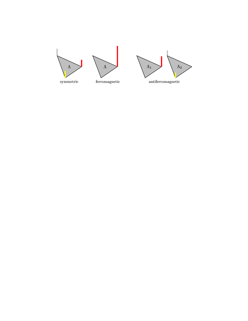
Figure 3: Single site distributions of the $3$-state Potts model.

3 Polyakov-loop dynamics

We consider pure Euclidean gauge theories with group valued link variables $U_{x;\mu}$ on a lattice with $N_{t}$ sites in the temporal direction. The fields are periodic in this direction, $U_{t+N_{t},\boldmathe{x};\mu}=U_{t,\boldmathe{x};\mu}$. We are interested in the distribution and expectation values of the traced Polyakov loop variable

$$L_{\boldmathe{x}}=\hbox{tr}\,{\cal P}{x},\qquad{\cal P}_{\boldmathe{x}}=\prod_{t=1}^{N_{t}}U_{t,\boldmathe{x};0},$$ (3.1)

since $\langle L{x}\rangle$ is an order parameter for finite temperature gluodynamics (see [13] for a review). In the low-temperature confined phase $\langle L_{\boldmathe{x}}\rangle=0$ and in the high-temperature deconfined phase $\langle L_{\boldmathe{x}}\rangle\neq 0$. The effective action for the Polyakov loop dynamics is

$$e^{-S_{\rm eff}[{\cal P}]}=\int{\cal D}U\delta\left({\cal P}_{\boldmathe{x}},\prod_{t=1}^{N_{t}}U_{t,\boldmathe{x};0}\right)\,e^{-S_{\rm w}[U]},\qquad{\cal D}U=\prod_{\rm links}d\mu_{\rm Haar}(U_{x;\mu}),$$ (3.2)

with gauge field action $S_{\rm w}$. In this formula the group valued field ${\cal P}{x}$ is prescribed and the delta-distribution enforces the constraints (3.1). In the simulations we used the Wilson action for the gauge fields. Gauge invariance of the action $S_{\rm w}[U]$ and measure ${\cal D}U$ implies $S_{\rm eff}[{\cal P}]=S_{\rm eff}[L]$. In addition there is the global center symmetry, under which all ${\cal P}{x}$ are multiplied by the same

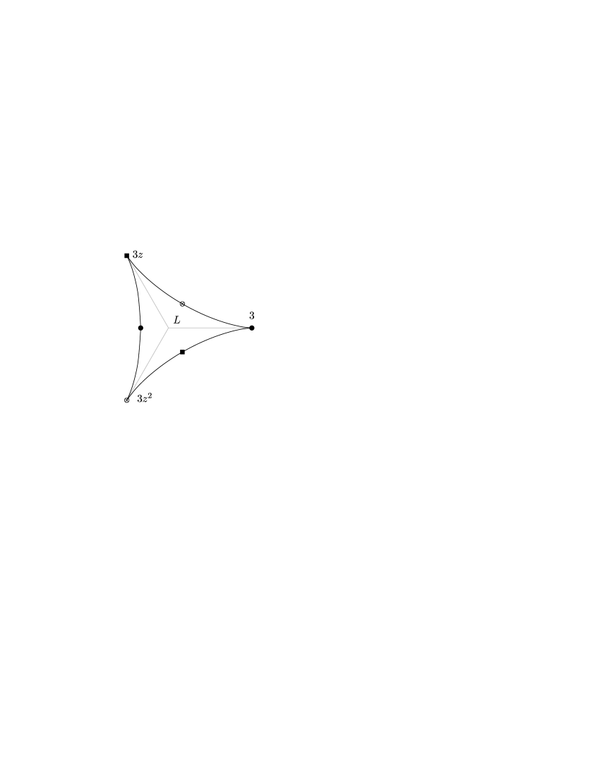
Figure 4: Fundamental domain of $L$.

center element of the group. For $SU(N)$ the center consists of the $N$ roots of unity, multiplied by the identity matrix. Hence for $SU(N)$ theories we have

$$S_{\rm eff}[L]=S_{\rm eff}[z\cdot L],\qquad z^{N}=1.$$

In Fig. 4 on the left we plotted the domain of the traced Polyakov loop variable for $SU(3)$. The values of $L$ at the three center elements are $3$, $3z$ and $3z^{2}$ with $z=e^{2\pi i/3}$. They form the edges of the triangle. What is needed is a good ansatz for the effective action $S_{\rm eff}$ in (3.2). To this aim we calculated the leading terms in the strong coupling expansion for $S_{\rm eff}$ in gluodynamics [2, 14]. As expected one finds a character expansion with nearest neighbor interactions,

$$S_{\rm eff}=\lambda_{10}S_{10}+\lambda_{20}S_{20}+\lambda_{11}S_{11}+\lambda_{21}S_{21}+\rho_{1}V_{1}+O(\beta^{3N_{t}}),$$

where $S_{pq}$ depends on the character $\chi_{pq}$ belonging to the representation $(p,q)$ of $SU(3)$. Expressing the characters as function of the fundamental characters $\chi_{10}=L$ and $\chi_{01}=L^{*}$ the different center-symmetric contributions have the form

$$S_{10}=\sum_{\langle\boldmathe{x}\boldmathe{y}\rangle}\left(L_{\boldmathe{x}}L_{\boldmathe{y}}^{*}+\text{h.c.}\right),$$

$$S_{20}=\sum_{\langle\boldmathe{x}\boldmathe{y}\rangle}\left(L_{\boldmathe{x}}^{2}L_{\boldmathe{y}}^{*2}-L_{\boldmathe{x}}^{2}L_{\boldmathe{y}}-L_{\boldmathe{x}}^{*}L_{\boldmathe{y}}^{*2}+L_{\boldmathe{x}}^{*}L_{\boldmathe{y}}+\text{h.c.}\right),$$

$$S_{11}=\sum_{\langle\boldmathe{x}\boldmathe{y}\rangle}\left(|L_{\boldmathe{x}}|^{2}|L_{\boldmathe{y}}|^{2}-|L_{\boldmathe{x}}|^{2}-|L_{\boldmathe{y}}|^{2}+1\right),$$

$$S_{21}=\sum_{\langle\boldmathe{x}\boldmathe{y}\rangle}\left(L_{\boldmathe{x}}^{2}L_{\boldmathe{y}}+L_{\boldmathe{y}}^{2}L_{\boldmathe{x}}-2L_{\boldmathe{x}}^{*}L_{\boldmathe{y}}+\text{h.c.}\right),\qquad V_{1}=\sum_{\boldmathe{x}}\left(|L_{\boldmathe{x}}|^{2}-1\right).$$

The target space for $L$ is the fundamental domain inside the triangle depicted above. The functional measure is not the product of Lebesgue measures but the product of reduced Haar measures on the lattice sites.

In the following we consider the two-coupling model

$$S_{\rm eff}=(\lambda_{10}-2\lambda_{21})\sum\left(L{x}L^{*}{y}+\hbox{h.c.}\right)+\lambda_{21}\sum\left(L{x}^{2}L{y}+L{y}^{2}L{x}+\hbox{h.c.}\right)$$ (3.3)

which contains the leading order contribution in the strong coupling expansion. For vanishing $\lambda_{21}$ it reduces to the Polonyi–Szlachanyi model [18].

4 Gluodynamics and Potts-model

There is a direct relation between the effective Polyakov loop dynamics and the $3$-state Potts model: If we freeze the Polyakov loops to the center of the group,

$${\cal P}{x}\longrightarrow z_{x}\mathbbm{1}\in\hbox{center}\big{(}SU(3)\big{)}\Longleftrightarrow\theta{x}\in\left\{0,\frac{2\pi}{3},\frac{4\pi}{3}\right\}$$

then the effective action (3.3) reduces to the Potts-Hamiltonian (2.1) with $J=18(\lambda_{10}+4\lambda_{21})$. The same reduction happens for all center-symmetric effective actions with nearest neighbor interactions. Only the relation between the couplings $\lambda_{pq}$ and $J$ is modified.

For the gauge group $SU(2)$ the finite temperature phase transition is second order and the critical exponents agree with those of the $2$-state Potts spin model which is just the ubiquitous Ising model. The following numbers are due to Engels et al. [15]

	$\beta/\nu$	$\gamma/\nu$	$\nu$
$4d$ SU(2)	$0.525$	$1.944$	$0.630$
$3d$ Ising	$0.518$	$1.970$	$0.629$

and support the celebrated Svetitsky–Yaffe conjecture [3]. For the gauge group $SU(3)$ the finite temperature phase transition is first order and we cannot compare critical exponents. But the effective theory (3.3) shows a second order transition from the symmetric to a antiferromagnetic phase and we can compare critical exponents at this transition with those of the same transition in the $3$-state Potts spin model.

In a first step we study the ‘classical phases’ of the Polyakov loop model with action (3.3). The classical analysis, where one minimizes the ‘classical action’ $S_{\rm eff}$, shows a ferromagnetic, antiferromagnetic and anticenter phase. The classical phase diagram is depicted in Fig. 5. For small couplings the quantum fluctuations will disorder the system and entropy will dominate energy. Thus we expect a symmetric phase near the origin in the $(\lambda_{10},\lambda_{21})$-plane and such a phase was inserted by hand in the diagram. There exists one unexpected phase which cannot exist for Potts spin models. It is an ordered phase for which the order parameter is near to the points opposite to the center elements, hence we call it anticenter phase. They are marked in the fundamental domain in Fig. 4. We shall see that the classical analysis yields the qualitatively correct phase diagram.

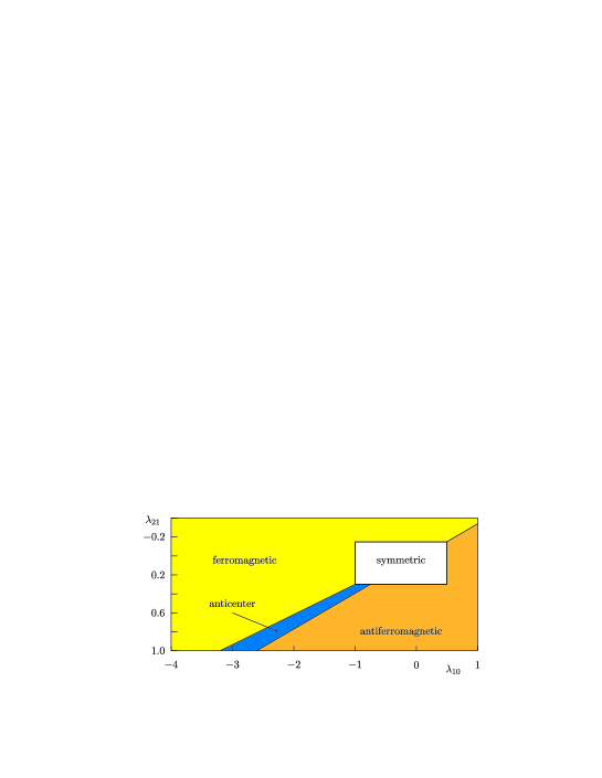
Figure 5: Classical phase diagram.

4.1 Modified mean field approximation

In a second step we calculate the effective potential for the Polyakov loop model with action (3.3) in the mean field approximation. Here we are not concerned with the relevance of this model for finite temperature gluodynamics and just consider (3.3) as the classical action of a field theoretical extension of the Potts spin models. We use the variational characterization (2.3) for the effective action where we must minimize with respect to probability measures on the space of field configuration $\{{\cal P}{x}|\boldmathe{x}\in\Lambda\}$ with fixed expectation values $\langle\chi_{pq}\rangle$ of all characters $\chi_{pq}({\cal P}{x})$ showing up in the Polyakov loop action. As outlined in Section 2, in the mean field approximation we assume the measures to have product form,

$${\cal DP}\longrightarrow\prod{x}d\mu_{\rm red}({\cal P}{x})\,p{x}\left({\cal P}{x}\right).$$

For further details the reader is referred to our earlier paper [17]. Here $\mu_{\rm red}$ is the reduced Haar measure of $SU(3)$. Since we expect an antiferromagnetic phase we only assume translational invariance on the sublattices in the decomposition (2.6). This way one arrives at a non-trivial variational problem on two sites.

We illustrate the procedure with the simple Polyakov loop model studied in [18],

$$S_{\rm eff}=\lambda S_{10}=\lambda\sum\left(L{x}L^{*}{y}+\hbox{h.c}\right).$$ (4.1)

To enforce the two constraints $\langle L{x}\rangle=L_{i}$ for $\boldmathe{x}\in\Lambda_{i}$ one introduces two Lagrangian multipliers. For the minimal model (4.1) one arrives at the following mean field effective potential

$$2u_{\rm mf}(L_{1},L_{1}^{*},L_{2},L_{2}^{*})=-d\lambda|L_{1}-L_{2}|^{2}+\sum v_{\rm mf}(L_{i},L_{i}^{*})$$

$$\hbox{with}\qquad v_{\rm mf}(L,L^{*})=d\lambda|L|^{2}+\gamma_{0}(L,L^{*}).$$

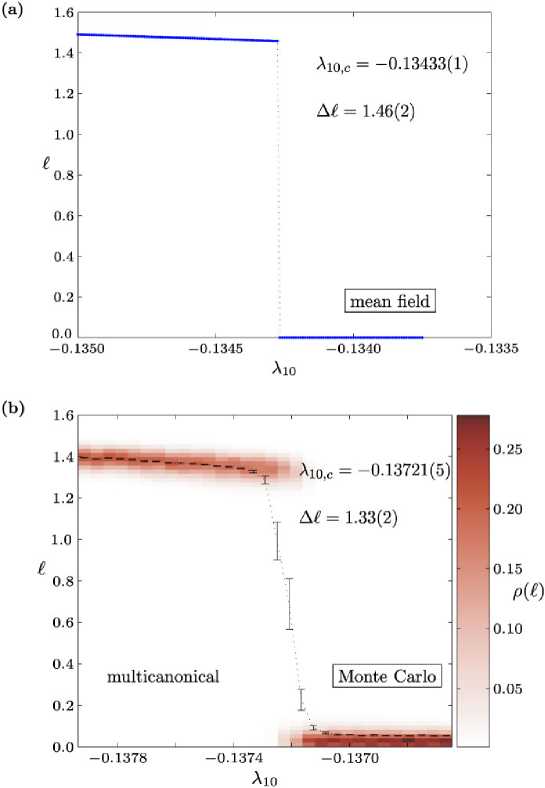
Figure 6: The order parameter $\ell$ for (a) mean field approximation and (b) Monte Carlo simulation.

Here $\gamma_{0}$ is the Legendre transform of

$$w_{0}(j,j^{*})=\log z_{0}(j,j^{*}),\qquad z_{0}(j,j^{*})={\int d\mu_{\rm red}\exp\left(jL+j^{*}L^{*}\right).}$$

The last integral has an expansion in terms of modified Bessel functions [19, 20],

$$z_{0}(j,j^{*})=\sum_{n\in\,\mbox{\af Z}}e^{inN\alpha}\,\det\begin{pmatrix}I_{n}&I_{n+1}&I_{n+2}\cr I_{n-1}&I_{n}&I_{n+1}\cr I_{n-2}&I_{n-1}&I_{n}\end{pmatrix}\left(2|j|\right),\qquad j=|j|e^{i\alpha}.$$

As order parameters discriminating the symmetric, ferromagnetic and antiferromagnetic phases we take [21]

$$L=\frac{1}{2}(L_{1}+L_{2}),\qquad M=\frac{1}{2}(L_{1}-L_{2}),\qquad\ell=|L|,\qquad m=|M|.$$ (4.2)

Fig. 6 shows the value of the order parameter $\ell$ as function of the coupling $\lambda_{10}$ near the phase transition point from the symmetric to the ferromagnetic phase. The value of the critical coupling and the jump $\Delta\ell$ of the order parameter in the mean field approximation and simulations agree astonishingly well. In Fig. 6b the order parameter $\ell$ for the ferromagnetic phase is plotted against its probability distribution given by the shaded area. In the vicinity of the first order transition we used a multicanonical algorithm on a $16^{3}$ lattice to calculate the critical coupling to very high precision. For further details on algorithmic aspects I refer to our recent paper [2]. Since the model has the same symmetries and dynamical degrees as the 3-state Potts model in 3 dimensions we expect the model to have a second order transition from the symmetric to the antiferromagnetic phase. To study this transition we calculated the order parameter $m$ in (4.2) in the modified mean field approximation and with Monte Carlo simulations. The order parameter $m$ is sensitive to the transition in question.

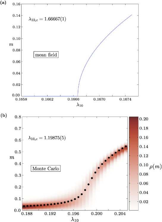
Figure 7: The order parameter $m$ for (a) mean field approximation and (b) Monte Carlo simulation.

Again the expectation value and probability distribution of $m$ near the transition is plotted in Fig. 7. To get a clear signal we have chosen a large lattice with $28^{3}$ sites and evaluated $5\times 10^{5}$ sweeps. The mean field approximation and Monte Carlo simulations together with the calculation of Binder cumulants in [2] indicate that the transition to the antiferromagnetic phase is second order. We plan to use a finite size scaling method to confirm this result in our upcoming work.

With the cumulant method we have calculated the critical exponents $\gamma$ and $\nu$ and compared our results with the same exponents for the $3$-state Potts model at the second order transition from the symmetric to the antiferromagnetic phase [21]. Within error bars the critical exponents are the same.

exponent	3-state Potts	minimal $S_{\rm eff}$
$\nu$	$0.664(4)$	$0.68(2)$
$\gamma/\nu$	$1.973(9)$	$1.96(2)$

This is how the conjecture relating finite temperature gluodynamics with spin models is at work: The Polyakov loop dynamics is effectively described by generalized Potts models with the fundamental domain as target space, for $SU(3)$ it is the triangularly shaped region in Fig. 4. The first order transition of gluodynamics is modelled by the transition from the symmetric to the ferromagnetic phase in the generalized Potts models. These generalized Potts models are in the same universality class as the ordinary Potts spin models; they have the same critical exponents at the ‘unphysical’ second order transition from the symmetric to the antiferromagnetic phase.

It is astonishing how good the mean field approximation is. The reason is probably, that the upper critical dimension of the (generalized) $3$-state Potts model is $3$ and not $4$ as one might expect. This is explained by the fact, that the models are embedded in systems with tricritical points, see below, and for such systems the upper critical dimension is reduced [22, 23].

5 Simulating the effective theories

We have undertaken an extensive and expensive scan to calculate histograms in the coupling constant plane $(\lambda_{10},\lambda_{21})$ of the model (3.3). Away from the transition lines we used a standard Metropolis algorithm giving results within 5 percent accuracy. Near first order transitions we simulated with a multicanonical algorithm on lattices with up to $20^{3}$ lattice sites. Most demanding have been the simulations near second order transitions. For that we developed a new cluster algorithm [2] which improved the auto-correlation times by two orders of magnitude on larger lattices. We found a rich phase structure with $4$ different phases with second and first order transitions and tricritical points. As for the minimal model the Monte Carlo simulations are in good and sometimes very good agreement with the mean field analysis.

Fig. 8 shows the phase structure in the generalized MF approximations and the corresponding results of our extended MC simulations. The results of the simulations are summarized in the following phase portrait (Fig. 9), in which we have indicated the order of the various transitions. The calculations were done on our Linux cluster with the powerful jenLaTT package. In $3000$ CPU hours we calculated $8000$ histograms in coupling constant space.

Figure 8: Phase structure for MF approximation and MC simulation.

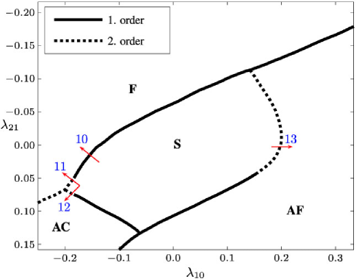
Figure 9: Phase portrait of the model (3.3). Histograms for the transitions are marked with arrows and figure numbers.

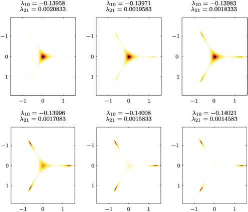
Figure 10: Histograms of $L$ which show a clear signal for the first order transition from the symmetric to the ferromagnetic phase.

For each marked transition in Fig. 9 a set of $6$ histograms is displayed. These histograms (and many others, see [2]) have been used to localize the phase transition lines and to investigate the nature of the transitions. The results are summarized in the phase portrait on page 9. The critical exponents $\nu$ and $\gamma$ given above have been determined at the second order transition indicated with arrow 13 in the portrait.

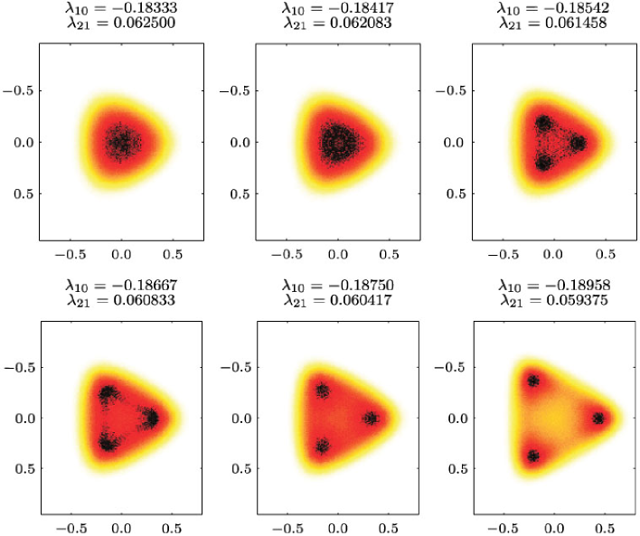
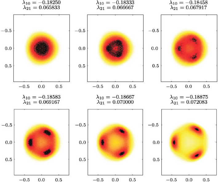
Figure 11: Histograms of $L$ for the continuous transition from the symmetric to the ferromagnetic phase.

Figure 12: Histograms of $L$ for the continuous transition from the symmetric to the anticenter phase.

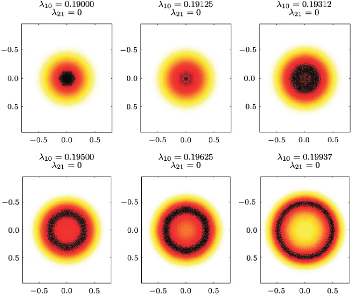
Figure 13: Histograms of $M$ for the second order transition from the symmetric to the antiferromagnetic phase.

6 Conclusion

The strong coupling expansion results in a character expansion for the Polyakov-loop dynamics. The leading terms are center symmetric nearest neighbor interactions containing the characters of the smallest representations of the gauge group. We have performed an extensive modified mean field analysis which includes antiferromagnetic states without translational invariance on the whole lattice. A new and efficient cluster algorithm has been developed and applied to study the second order transitions from the symmetric to the antiferromagnetic phase. The autocorrelation times were improved by $2$ orders of magnitude. We discovered an unexpectedly rich phase structure of the simple $2$-coupling Polyakov loop model (3.3). This model is in the same universality class as the $3$-state Potts spin model. The mean field results are surprisingly accurate that seems to indicate that the upper critical dimension of the generalized Potts models is $3$. This is attributed to the existence of tricritical points [22, 23].

To relate our results to gluodynamics we have to calculate the effective couplings $\lambda_{pq}$ governing Polyakov-loop dynamics as functions of the Wilson coupling $\beta$ in gluodynamics. We have done this successfully for $SU(2)$ gauge theory with inverse Monte Carlo techniques [17, 24] and plan to publish our results for $SU(3)$ very soon [25]. For the inverse Monte Carlo simulations to work one needs simple geometric Schwinger Dyson equations for the Polyakov loop dynamics. Such equations have been derived very recently in [20]. It would be interesting to see whether the antiferromagnetic phase of the Polyakov loop models plays any role at all for gluodynamics. In the present paper it was needed to show that certain critical exponents of the Polyakov loop models are the same as of the $q=3$ Potts spin model. Finally one would like to include heavy fermions in the effective Polyakov-loop dynamics [26]. To that end one needs to add center symmetry breaking terms to the effective actions studied in the present paper. This will lead to a proliferation of additional terms in the effective action which renders a systematic study more difficult as compared to pure gluodynamics.

Acknowledgements

Andreas Wipf would like to thank the local organizing committee of the O’Raifeartaigh Symposium on Non-Perturbative and Symmetry Methods in Field Theory for organizing such a stimulating and pleasant meeting on the hills of Budapest to commemorate Lochlainn O’Raifeartaigh and his important contributions to physics. This contribution is very much in the tradition of his research on the role of symmetries and effective potentials in field theory.

References

- [1]
- [2] Wozar C., Kaestner T., Wipf A., Heinzl T., Pozsgay B., Phase structure of -Polyakov-loop models, Phys. Rev. D 74 (2006), 114501, 19 pages, hep-lat/0605012.
- [3] Yaffe L.G., Svetitsky B., First order phase transition in the gauge theory at finite temperature, Phys. Rev. D 26 (1982), 963–965.
- [4] Bazavov A., Berg B.A., Velytsky A., Glauber dynamics of phase transitions: lattice gauge theory, Phys. Rev. D 74 (2006), 014501, 12 pages, hep-lat/0605001.
- [5] Ashkin J., Teller E., Statistics of two-dimensional lattices with four components, Phys. Rev. 64 (1942), 178–184.
- [6] Potts R.B., Some generalized order-disorder transformations, Proc. Camb. Phil. Soc. 48 (1952), 106–109.
- [7] Wu F.Y., The Potts model, Rev. Modern Phys. 54 (1982), 235–268.
- [8] Yamaguchi C., Okabe Y., Three-dimensional antiferromagnetic -state Potts models: application of the Wang–Landau algorithm, J. Phys. A: Math. Gen. 34 (2001), 8781–8794, cond-mat/0108540.
- [9] Harris A.B., Mouritsen O.G., Berlinsky A.J., Pinwheel and herringbone structures of planar rotors with anisotropic interactions on a triangular lattice with vacancies, Can. J. Phys. 62 (1984), 915–934.
- [10] Roepstorff G., Path integral approach to quantum physics, Springer, 1994.
- [11] O’Raifeartaigh L., Wipf A., Yoneyama H., The constraint effective potential, Nuclear Phys. B 271 (1986), 653–680.
- [12] Fujimoto Y., Yoneyama H., Wipf A., Symmetry restoration of scalar models at finite temperature, Phys. Rev. D 38 (1988), 2625–2634.
- [13] Holland K., Wiese U.-J., The center symmetry and its spontaneous breakdown at high temperatures, in At the Frontier of Particle Physics – Handbook of QCD, Vol. 3, Editor M. Shifman, World Scientific, Singapore, 2001, 1909–1944, hep-ph/0011193.
- [14] Buss G., Analytische Aspekte effektiver -Gittereichtheorien, Diploma Thesis, Jena, 2004.
- [15] Engels J., Mashkevich S., Scheideler T., Zinovjev G., Critical behaviour of lattice gauge theory. A complete analysis with the -method, Phys. Rev. B 365 (1996), 219–224, hep-lat/9509091.
- [16] Gliozzi F., Necco S., Critical exponents for higher-representation sources in gauge theory from CFT, hep-th/0605285.
- [17] Heinzl T., Kaestner T., Wipf A., Effective actions for the confinement-deconfinement phase transition, Phys. Rev. D 72 (2005), 065005, 14 pages, hep-lat/0502013.
- [18] Polonyi J., Szlachanyi K., Phase transition from strong coupling expansion, Phys. Lett. B 110 (1982), 395–398.
- [19] Carlsson J., McKellar B., Glueball masses in 2+1 dimensions, Phys. Rev. D 68 (2003), 074502, 18 pages, hep-lat/0303016.
- [20] Meinel R., Uhlmann S., Wipf A., Ward identities for invariant group integrals, hep-th/0611170.
- [21] Wang J.S., Swendsen R.H., Kotecky R., Three-state antiferromagnetic Potts models: a Monte Carlo study, Phys. Rev. B 42 (1990), 2465–2474.
- [22] Lawrie I., Sarbach S., Theorie of tricritical points, in Phase Transitions and Critical Phenomena, Vol. 9, Editors C. Domb and J. Lebowitz, Academic Press, 1984, 2–155.
- [23] Landau D., Swendsen R., Monte Carlo renormalization-group study of tricritical behavior in two dimensions, Phys. Rev. B 33 (1986), 7700–7707.
- [24] Dittmann L., Heinzl T., Wipf A., An effective lattice theory for Polyakov loops, JHEP 0406 (2004), 005, 27 pages, hep-lat/0306032.
- [25] Heinzl T., Kaestner T., Wipf A., Wozar C., effective Polyakov-loop dynamics, in preparation.
- [26] Kim S., de Forcrand Ph., Kratochvila S., Takaishi T., The 3-state Potts model as a heavy quark finite density laboratory, PoSLAT2005, 2006, 166, 6 pages, hep-lat/0510069.