Finite temperature phase transition of two-flavor QCD with an improved Wilson quark action

Abstract:

We study the phase structure of QCD at finite temperatures with two flavors of dynamical quarks on a lattice with the size $N_{s}^{3}\times N_{t}=16^{3}\times 4$, using a renormalization group improved gauge action and a clover improved Wilson quark action. The simulations are made along the lines of constant physics determined in terms of $m_{\rm PS}/m_{\rm V}$ at zero-temperature. We show prelimnary results for the spatial string tension in the high temperature phase.

1 Introduction

Recent relativistic heavy ion collision experiments have revealed various remarkable properties of QCD at finite temperatures and densities, suggesting the realization of the QCD phase transition from the hadronic matter to the quark-gluon plasma (QGP). In order to extract an unambiguous signal for the transition from the heavy ion collision experiments, it is indispensable to make quantitative calculation of the thermal properties of QGP from first principles. Currently, the lattice QCD simulation is the only systematic method to do so. By now, most of the lattice QCD studies at finite temperature and chemical potential have been performed using staggered-type quarks which require less computational costs than others. However, the lattice artifacts of the staggered-type quarks are not fully understood. Therefore, it is important to compare the results from other lattice quarks to control and estimate the lattice discretization errors.

We have started systematic studies of finite temperature/density QCD using Iwasaki’s RG-improved gauge action [1] and a clover-improved Wilson quark action [2]. In particular, we perform simulations along the lines of constant physics (LCP’s) to clearly extract the temperature- and density-dependences. As the first project in this direction, we are carrying out simulations of $N_{f}=2$ QCD on an $N_{s}^{3}\times N_{t}=16^{3}\times 4$ lattice at $m_{\rm PS}/m_{\rm V}=0.65$ and 0.80 in the range $T/T_{pc}\sim 0.76$–3.2, where $T_{pc}$ is the pseudocritical point along the LCP. Basic properties of the system at finite temperatures, such as the phase structure and the equation of state, have been studied in [3, 4]. In contrast to the studies with the staggered-type quarks, the expected $O(4)$ scaling for $N_{f}=2$ QCD was confirmed. We extend the study to analyse detailed properties of QGP at finite temperature and chemical potential.

In this paper, we report on the status of our simulations and present a preliminary result for the spatial string tension at finite temperature. Results for the free energies of static quarks at zero chemical potential are presented in [5]. Preliminary results of the equation of state and susceptibilities at non-zero chemical potential by the Taylor expansion method are given in [6].

2 Lattice action

We employ the RG-improved gauge action [1] and the $N_{f}=2$ clover-improved Wilson quark action [2] defined by

$$S=S_{g}+S_{q},$$ (1)

$$S_{g}=-{\beta}\sum_{x}\left(c_{0}\sum_{\mu<\nu;\mu,\nu=1}^{4}W_{\mu\nu}^{1\times 1}(x)+c_{1}\sum_{\mu\neq\nu;\mu,\nu=1}^{4}W_{\mu\nu}^{1\times 2}(x)\right),$$ (2)

$$S_{q}=\sum_{f=1,2}\sum_{x,y}\bar{q}_{x}^{f}D_{x,y}q_{y}^{f},$$ (3)

where $\beta=6/g^{2}$, $c_{1}=-0.331$, $c_{0}=1-8c_{1}$ and

$$D_{x,y}=\delta_{xy}-{K}\sum_{\mu}\{(1-\gamma_{\mu})U_{x,\mu}\delta_{x+\hat{\mu},y}+(1+\gamma_{\mu})U_{x,\mu}^{\dagger}\delta_{x,y+\hat{\mu}}\}-\delta_{xy}{c_{SW}}{K}\sum_{\mu>\nu}\sigma_{\mu\nu}F_{\mu\nu}.$$ (4)

Here $K$ is the hopping parameter, $F_{\mu\nu}$ is the lattice field strength with $f_{\mu\nu}$ the standard clover-shaped combination of gauge links, $F_{\mu\nu}={1}/{8i}(f_{\mu\nu}-f^{\dagger}_{\mu\nu})$. For the clover coefficient $c_{SW}$, we adopt a mean field value using $W^{1\times 1}$ which was calculated in the one-loop perturbation theory [1],

$${c_{SW}}=(W^{1\times 1})^{-3/4}=(1-0.8412\beta^{-1})^{-3/4}.$$ (5)

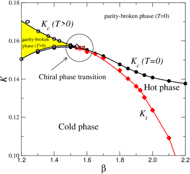
Figure 1: Phase diagram for RG improved gauge action and clover improved Wilson quark action for $N_{t}=4$.

The phase diagram of this action in the $(\beta,K)$ plane has been obtained by the CP-PACS Collaboration [3, 4] as shown in Fig.1. The solid line $K_{c}(T=0)$ with filled circles is the chiral limit where pseudoscalar mass vanishes at zero temperature. Above the $K_{c}(T=0)$ line, the parity-flavor symmetry is spontaneously broken. At finite temperatures, the cusp of the parity-broken phase retracts from the large $\beta$ limit to a finite $\beta$. The solid line $K_{c}(T>0)$ connecting open symbols represents the boundary of the parity-broken phase. The red line $K_{t}$ represents the finite temperature pseudocritical line determined from the peak of Polyakov loop susceptibility. This line separates the hot phase (the quark-gluon plasma phase) and the cold phase (the hadron phase). The crossing point of the $K_{t}$ and the $K_{c}(T=0)$ lines is the chiral phase transition point.

3 Determination of lines of constant physics and simulation parameters

For phenomenological applications, we need to investigate the temperature dependence of thermodynamic observables on a line of constant physics (LCP), which we determine by the ratio $m_{\rm PS}/m_{\rm V}$ of pseudoscalar and vector meson masses. For our purpose, we need LCP in a wider range of parameters than [4]. Therefore, we re-analyze the data for $m_{\rm PS}a$ and $m_{\rm V}a$ at zero temperature shown in Fig.2 determined by the CP-PACS Collaboration [3, 4, 7, 8]. The colored solid lines in Fig.3 shows our results for LCP corresponding to $m_{\rm PS}/m_{\rm V}=0.65,0.70,0.75,0.80,0.85,0.90$ and $0.95$. The green line denoted as $K_{c}$ represents the critical line, i.e. $m_{\rm PS}/m_{\rm V}=0$. Our LCP’s are consistent with those of [4] in the range of the previous study.

Figure 2: Pseudoscalar meson mass squared (left) and vector meson mass (right) as a function of $1/K$ for several values of $\beta$ at $T=0$.

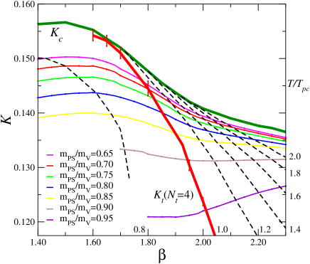
Figure 3: Lines of constant $m_{\rm PS}/m_{\rm V}$ and constant $T/T_{ps}$ in the $(\beta,K)$ plane.

We also reanalyze the lines of constant temperature $T/T_{pc}$. The temperature $T$ is estimated by the zero-temperature vector meson mass $m_{\rm V}a(\beta,K)$ using

$$\frac{T}{m_{\rm V}}(\beta,K)=\frac{1}{N_{t}\times m_{\rm V}a(\beta,K)}.$$ (6)

The lines of constant $T/T_{pc}$ is determined as the ratio of ${T}/{m_{\rm V}}$ to ${T_{pc}}/{m_{\rm V}}$ where $T_{pc}/m_{\rm V}$ is obtained by $T/m_{\rm V}$ at $K_{t}$ on the same LCP. The bold red line denoted as $K_{t}(N_{t}=4)$ in Fig.3 represents the pseudocritical line $T/T_{pc}=1$. The dashed lines represent the results for $T/T_{pc}=0.8,1.2,1.4,1.6,1.8,2.0$ at $N_{t}=4$.

We perform finite temperature simulations on a lattice with a temporal extent $N_{t}=4$ and a spatial extent $N_{s}=16$ along the LCP’s for $m_{\rm PS}/m_{\rm V}=0.65$ and $0.80$. The standard hybrid Monte Carlo algorithm is employed to generate full QCD configurations with two flavors of dynamical quarks. The length of one trajectory is unity and the molecular dynamics step size is tuned to achieve an acceptance rate greater than about 70%. Runs are carried out in the range $\beta=1.50$–2.30 at twelve values of $T/T_{pc}\sim 0.82-3.2$ for $m_{\rm PS}/m_{\rm V}=0.65$ and eleven values of $T/T_{pc}\sim 0.76-2.5$ for $m_{\rm PS}/m_{\rm V}=0.80$. Our simulation parameters and the corresponding temperatures are summarized in Table 1. The number of trajectories for each run after thermalization is $5000-6000$. We measure physical quantities at every 10 trajectories.

Table 1: Simulation parameters for $m_{\rm PS}/m_{\rm V}=0.80$ (left) and $m_{\rm PS}/m_{\rm V}=0.65$ (right).

$\beta$	$K$	$T/T_{pc}$	Traj.
1.50	0.143480	0.76446	5500
1.60	0.143749	0.79544	6000
1.70	0.142871	0.84346	6000
1.80	0.141139	0.92507	6000
1.85	0.140070	0.98642	6000
1.90	0.138817	1.07619	6000
1.95	0.137716	1.19836	6000
2.00	0.136931	1.34778	5000
2.10	0.135860	1.69025	5000
2.20	0.135010	2.07325	5000
2.30	0.134194	2.51093	5000

$\beta$	$K$	$T/T_{pc}$	Traj.
1.50	0.150290	0.82434	5000
1.60	0.150030	0.86471	5000
1.70	0.148086	0.94442	5000
1.75	0.146763	1.00024	5000
1.80	0.145127	1.07466	5000
1.85	0.143502	1.17857	5000
1.90	0.141849	1.31675	5000
1.95	0.140472	1.48262	5000
2.00	0.139411	1.66828	5000
2.10	0.137833	2.09054	5000
2.20	0.136596	2.59279	5000
2.30	0.135492	3.21536	5000

4 Spatial Wilson Loop

Using the stored configurations, we are carrying out a series of studies on the nature of the quark-gluon plasma. In this report, we present our preliminary results on the confinement in the spatial directions at high temperature.

In previous quenched studies[9, 10, 11, 12], Wilson loops in spatial directions are found to show non-vanishing spatial string tension $\sigma_{s}$ even at $T>T_{pc}$, which is called the spatial confinement. We study this phenomenon when there exist dynamical quarks in the system. Altough quarks are expected to decouple from the spatial observables for $T\gg T_{pc}$ due to dimensional reduction and thus do not affect $\sigma_{s}$ in the high temperature limit, it is not obvious whether the same is true near $T_{pc}$.

As a first trial, we evaluate $\sigma_{s}$ assuming the simplest ansatz for the spatial Wilson loops $W(I,J)$ with the size $I\times J$:

$$-\ln W(I,J)=\sigma_{s}IJ+\sigma_{peri}(2I+2J)+C_{w},$$ (7)

where $\sigma_{s}$, $\sigma_{peri}$ and $C_{w}$ are fit parameters. The results for $\sqrt{\sigma_{s}(T)}/T_{pc}$ are shown in Fig.4 as a function of $T/T_{pc}$. We find that $\sqrt{\sigma_{s}(T)}/T_{pc}$ tends to a non-vanishing value below $T_{pc}$ while it increases linearly in $T/T_{pc}$ above $T_{pc}$. Similar behavior was observed in the quenched case too [9].

Let us now compare the results with a calculation of $\sqrt{\sigma_{s}}$ by the three-dimensional effective theory assuming the dominance of the gauge part. We would expect the following behaviour for the spatial string tension,

$${\sqrt{\sigma_{s}(T)}} = c\ g^{2}(T)\ T,$$ (8)

where $g^{2}(T)$ is the two-loop temperature dependent running coupling constant in four dimensions,

$$g^{-2}(T)=\frac{29}{48\pi^{2}}\ln\frac{T}{\Lambda}+\frac{226}{768\pi^{4}}\ln\left(2\ln\frac{T}{\Lambda}\right).$$ (9)

We carry out a fit to our data shown in Fig.4, regarding $c$ and $\Lambda$ free parameters. From the two parameter fit, we find

$$c=0.54(6),\ \ \Lambda/T_{pc}=0.14(4).$$ (10)

We note that these values are similar to those obtained in a quenched study [11, 12]: $c=0.566(13)$ and $\Lambda/T_{pc}=0.104(9)$.

We also note that there is a parameter-free three-dimensional effective theory prediction for $\sqrt{\sigma_{s}(T/T_{pc},T_{pc}/\Lambda_{\overline{\rm MS}},\overline{\mu}/T)}$ [13], where $\overline{\mu}$ is the $\overline{{\rm MS}}$ scheme scale parameter. The $\overline{\mu}/T$ is fixed as in [13]. We vary the value of $T_{pc}/\Lambda_{\overline{\rm MS}}$ in the range $0.53-0.77$ [3, 14]. The results for $\sqrt{\sigma_{s}}/T$ are compared with our data in Fig.5. While the 1-loop prediction of the effective theory (shown by the region bounded by two green lines in Fig.5) deviates from the lattice data, the 2-loop result (shown by the region bounded by two black lines) is roughly consistent with our data. A more detailed test is left for a future work.

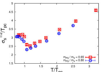
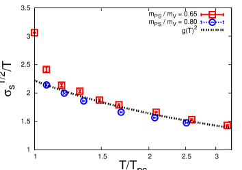
Figure 4: The square root of the spatial string tension over $T_{pc}$ (left) and $T$ (right) as a function of $T/T_{pc}$ for $m_{\rm PS}/m_{rmV}=0.65,0.80$. The dashed line (right) shows the two-loop fit.

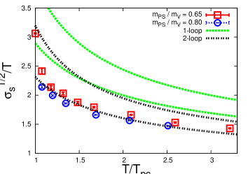
Figure 5: Comparison of our data and 1-loop and 2-loop predictions from three-dimensional effective theory. $\overline{\mu}/T$ is fixed as in [13]. $T_{pc}/\Lambda_{\overline{\rm MS}}$ is varied in the range $0.53-0.77$.

5 Conclusions

Most of the lattice QCD studies at finite temperatures and densities have been done using staggered-type quarks. To control the lattice artifacts, comparisons with other lattice quarks are indispensable. Therefore, we have started a systematic study of QCD at finite temperature and density with an improved Wilson quark action.

As a first step, we performed simulations of $N_{f}=2$ QCD on an $N_{s}^{3}\times N_{t}=16^{3}\times 4$ lattice. We have identified the lines of constant physics and studied the temperature-dependence of various quantities at $m_{\rm PS}/m_{\rm V}=0.65$ and 0.80 in the range $T/T_{pc}\sim 0.76$–3.2. A preliminary result of the spatial string tension $\sigma_{s}(T)$ in the quark-gluon plasma shows a behavior consistent with ${\sqrt{\sigma_{s}(T)}}=c\ g^{2}(T)\ T$ where $c$ takes a value close to that in the quenched case (gluon plasma). $\sigma_{s}(T)$ is also consistent with the parameter-free prediction of the three-dimensional effective theory in the 2-loop order. Further results on the static quark free energies at finite temperatures for different color channels are given in [5]. Results on the equation of state and susceptibilities at non-zero chemical potential with Wilson-type quarks are shown in [6].

Acknowledgements:

This work is supported by Grants-in-Aid of the Japanese Ministry of Education, Culture, Sports, Science and Technology, (Nos. 13135204, 15540251, 17340066, 18540253, 18740134). SE is supported by Sumitomo Foundation (No. 050408), and YM is supported by JSPS. This work is in part supported also by the Large-Scale Numerical Simulation Projects of ACCC, Univ. of Tsukuba, and by the Large Scal Simulation Program of High Energy Accelerator Research Organization (KEK).

References

- [1] Y. Iwasaki, Nucl. Phys. B 258, 141 (1985); University of Tsukuba Report No. UTHEP-118 (1983).
- [2] B. Sheikholeslami and R. Wohlert, Nucl. Phys. B 259, 572 (1985).
- [3] CP-PACS Collaboration, A. Ali Khan et al., Phys. Rev. D 63, 034502 (2000).
- [4] CP-PACS Collaboration, A. Ali Khan et al., Phys. Rev. D 64, 074510 (2001).
- [5] Y. Maezawa et al., PoS LAT2006, 141.
- [6] S. Ejiri et al., PoS LAT2006, 132.
- [7] CP-PACS Collaboration, A. Ali Khan et al., Phys. Rev. Lett. 85, 4674 (2000).
- [8] CP-PACS Collaboration, A. Ali Khan et al., Phys. Rev. D 65, 054505 (2001).
- [9] G. S. Bali et al., Phys. Rev. Lett. 71, 3059 (1993).
- [10] L. Kärkkäinen et al., Phys. Lett. B 312, 173 (1993).
- [11] F. Karsch et al., Phys. Lett. B 346, 94 (1995).
- [12] G. Boyd et al., Nucl. Phys. B 469, 419 (1996).
- [13] Y. Schröder and M. Laine, PoS LAT2005, 180 (2006).
- [14] M. Gockeler et al., Phys. Rev. D 73, 04506 (2004).