About Orientifold Planar Equivalence on the Lattice

Abstract:

The orientifold planar equivalence is the equivalence in the large-$N$ limit of the bosonic sectors of the super Yang-Mills and the QCD with a quark in the antisymmetric representation. I give a sketch of the proof of the orientifold planar equivalence in the strong-coupling and large-mass phase on the lattice. It is still matter of discussion, if its validity extends also in the continuum limit.

1 Large-N limits of QCD

The idea behind the orientifold planar expansion is an old one. Because of its inherent non-perturbative features, QCD is a very hard theory to solve. However, one can approximate QCD with some other (possibly simpler) theory, in order to obtain analytical, if approximate, predictions. Real QCD is an $SU(3)$ gauge theory with six quarks in the fundamental representation, each one with a well-defined non-zero mass. Therefore, theories that approximate real QCD can be built by slightly changing some parameters. For instance, it is found that changing the number of colours and studying the large-$N$ (or planar) limit can lead to an acceptable approximation. One can also change other parameters, like the masses of the up and down quarks, as the chiral limit is very interesting to study.

In order to compute a large-$N$ limit, one needs to define a multicoloured version of QCD. Usually, one chooses an $SU(N)$ gauge theory with quarks in the fundamental representation, where the coupling constant $g^{2}$ is replaced by $\lambda/N$. When the number of colours approaches infinity, this theory becomes quenched, that is a pure gauge theory with quarks behaving as classical external sources.

This is not the only way to generalise QCD to the case of $N$ colours. Consider the following simple fact: the antifundamental representation of $SU(3)$ is the same as the antisymmetric one. In fact, thanks to the invariance of the fully skew-symmetric $\epsilon_{ijk}$ tensor, a one-to-one map between the two representations exists.

$$\bar{q}_{i}=\frac{1}{2}\epsilon_{ijk}Q^{jk}\qquad Q^{jk}=\epsilon^{ijk}\bar{q}_{i}$$

$$\bar{q}\rightarrow U^{*}\bar{q}\quad\mbox{iff}\quad Q\rightarrow UQU^{T}$$ (1)

Thus, the multicoloured QCD can be alternatively defined as an $SU(N)$ gauge theory with quarks in the antisymmetric representation (the coupling constant $g^{2}$ must be replaced by $\lambda/N$ in this case, too). In what follows, I will refer to this theory as orientifold QCD. Now the question is: what is the planar limit of orientifold QCD?

In the case of one massless flavour (but this result can be extended to the case of more than one flavours), Armoni, Shifman and Veneziano proposed that orientifold QCD is equivalent to super Yang-Mills in the planar limit [1, 2, 3]. This conjecture in known as orientifold planar equivalence.

In the class of strong-interacting theories, the supersymmetric ones play a unique role. In fact, thanks to supersymmetry, some non-perturbative quantities can be analytically computed. If the orientifold planar equivalence holds, the corresponding quantities in QCD can be estimated up to $1/N$-corrections. This is the case, for example, of the chiral condensate in QCD, that can be estimated from the gluino condensate in SYM, obtaining a value consistent with the numerical simulations [4, 5].

At the present, the validity of the orientifold planar equivalence is matter of controversy. Armoni, Shifman and Veneziano claimed to have provided a rigorous proof of this conjecture [6]. In a recent work, Unsal and Yaffe assert that a dynamical condition was missing in the proof: the equivalence holds if and only if the charge conjugation symmetry is not spontaneously broken in orientifold QCD [7].

In the future, we could get hints from numerical simulations about the validity of the orientifold planar equivalence. Computationally, this is a very hard problem. In fact, simulating a gauge theory with fermions in a two-indices representation (the dimension of the representation grows like $N^{2}$) has a time cost growing roughly like $N^{6}$. (Whilst, for a pure gauge theory the simulation time grows roughly like $N^{3}$.) Deferring this problem to future studies, it is interesting to understand what it is possible to assert about orientifold planar equivalence between lattice-discretized theories.

In this paper, I will give a sketch of the proof of orientifold planar equivalence on the lattice in the phase of strong coupling and large fermionic mass. A detailed version of this proof is available in [8].

2 Planar equivalence on the lattice

Let us focus on the following two theories on the lattice:

AdjQCD.

Gauge theory with one Majorana fermion of mass $m$ in the adjoint representation.

AsQCD.

Gauge theory with one Dirac fermion of mass $m$ in the antisymmetric two-indices representation.

In what follows, I use the Wilson discretization for the Dirac operator

$$D_{xy}=\delta_{xy}-\kappa\sum_{\mu}\left\{(r_{0}-\gamma_{\mu})R[U_{\hat{\mu}}(x)]\delta_{x+\hat{\mu},y}+(r_{0}+\gamma_{\mu})R[U_{-\hat{\mu}}(x)]\delta_{x-\hat{\mu},y}\right\}$$ (2)

where $\kappa$ is the hopping parameter and $R$ is the appropriate representation which the fermions belong to. The Majorana fermion is defined by introducing the square root of the fermionic determinant in the partition function. Thus the (not normalized) statistical weights of the gauge configurations are

$$\rho_{\textrm{Adj}}(U)\;\mathcal{D}U=e^{-S_{W}(U)}\;\det{D_{\textrm{Adj}}(U)}^{\frac{1}{2}}\;\mathcal{D}U$$

$$\rho_{\textrm{As}}(U)\;\mathcal{D}U=e^{-S_{W}(U)}\;\det D_{\textrm{As}}(U)\;\mathcal{D}U$$ (3)

for the two theories, where $S_{W}(U)$ is the Wilson action for the gauge field.

In the next Section, I will prove that the expectation value of a product of Wilson loops has the same large-$N$ limit in the two theories, in the framework of large-coupling and large-mass expansion. More precisely, if $\left\{\mathcal{W}_{i}\right\}$ are Wilson loops on the lattice, one has that

$$\lim_{N\rightarrow\infty}\frac{1}{N^{k}}\left<\mathcal{W}_{1}\cdots\mathcal{W}_{k}\right>_{\textrm{Adj}}=\lim_{N\rightarrow\infty}\frac{1}{N^{k}}\left<\mathcal{W}_{1}\cdots\mathcal{W}_{k}\right>_{\textrm{As}}$$ (4)

where the equality holds for each term of the expansion of both the expectation values as a power series in $\lambda^{-1}$ and $\kappa$.

3 Planar limit in the strong-coupling and large-mass phase

As a first step, let us perform the hopping expansion of the fermionic effective action (for the details, see [9]):

$$S_{F}=-\log\det D_{R}^{N_{f}}=N_{f}\sum_{\alpha\in\mathcal{C}}\kappa^{L(\alpha)}c(\alpha)\mathcal{W}_{R}(\alpha)$$ (5)

where $\mathcal{C}$ is the set of all the closed paths linking nearest neighbours on the lattice, $L(\alpha)$ is the length of the path $\alpha$, $\mathcal{W}_{R}(\alpha)$ is the Wilson loop along the path $\alpha$ in the representation $R$, $c(\alpha)$ is a representation-independent coefficient and $N_{f}$ is $1$ for AsQCD or $1/2$ for AdjQCD.

Using standard relations, Wilson loops in the adjoint and antisymmetric representations can be written in terms of Wilson loops in the (anti-)fundamental representations:

$$\frac{1}{2}\mathrm{tr}\,\textbf{Adj}(U)=\frac{1}{2}\left\{\left|\mathrm{tr}U\right|^{2}-1\right\}\simeq\frac{1}{2}\left|\mathrm{tr}U\right|^{2}$$

$$\mathrm{tr}\,\textbf{As}(U)=\frac{1}{2}\left\{\left(\mathrm{tr}U\right)^{2}-\mathrm{tr}U^{2}\right\}\simeq\frac{1}{2}\left(\mathrm{tr}U\right)^{2}\;.$$ (6)

Here, the approximations are valid in the planar limit.

Putting all together, the actions of the two theories can be written as:

$$S_{\textrm{Adj}}(U)\simeq\frac{2N^{2}}{\lambda}\sum_{p}\left(1-\frac{1}{N}\textrm{Re}\,\mathrm{tr}\,U_{p}\right)+\frac{1}{2}\sum_{\alpha\in\mathcal{C}}\kappa^{L(\alpha)}c(\alpha)\left|\mathrm{tr}\mathcal{W}(\alpha)\right|^{2}$$

$$S_{\textrm{As}}(U)\simeq\frac{2N^{2}}{\lambda}\sum_{p}\left(1-\frac{1}{N}\textrm{Re}\,\mathrm{tr}\,U_{p}\right)+\frac{1}{2}\sum_{\alpha\in\mathcal{C}}\kappa^{L(\alpha)}c(\alpha)\left(\mathrm{tr}\mathcal{W}(\alpha)\right)^{2}$$ (7)

where $\mathcal{W}(\alpha)$ is the Wilson loop along $\alpha$ in the fundamental representation. It is clear that the orientifold planar equivalence is based on the possibility of reversing the orientation of one of the two Wilson loops coming from the fermionic effective action. The full strong-coupling and large- mass expansion of the statistical weights in (2) is obtained by expanding the exponential $e^{-S}$ as a power series.

In order to compute the partition function, one can replace the exponential in the integral with its power series, and fully expand each of the terms. The partition function is finally obtained as a sum of graphs.

Each graph is an integral over all the link variables of a product of some plaquettes (times $2N/\lambda$) coming from the Wilson action and some couples of Wilson loops (times $\kappa^{L(\alpha)}c(\alpha)/2$) coming from the fermionic effective action. It can be shown [10] that at leading order in $1/N$ the effect of the integration over the gauge group is to perform Wick-contractions between couples of $U$ and $U^{\dagger}$:

$$U_{ij}U^{*}_{kl}\rightarrow\frac{1}{N}\delta_{ik}\delta_{jl}\;.$$ (8)

As a consequence, we can use all the machinery developed for the usual perturbation theory. For example, the expectation value of a Wilson loop is given by the sum of all the “connected graphs” (times the appropriate combinatorial factor) with the insertion of the Wilson loop. The “connected graphs” are those which cannot be written as a product of two other graphs of the theory.

A graph can be represented as a possibly disconnected surface bounded by Wilson loops and tiled by plaquettes, that are sewn by Wick-contractions (see figure 1).

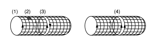
Figure 1: On the left, a graph of the expectation value of a WIlson loop for AdjQCD. On the right, a similar graph for AsQCD. (1) Inserted Wilson loop. (2) Plaquette. (3) $\left(\mathrm{tr}U\right)^{2}$ from a Wilson loop in the antisymmetric representation (from the fermionic determinant). (4) $\left|\mathrm{tr}U\right|^{2}$ from a Wilson loop in the adjoint representation (from the fermionic determinant).

As in the usual ’t Hooft expansion [11], graphs are proportional to $N^{\chi}$, where $\chi$ is the Euler characteristic of the surface:

$$\chi=2C-2H-B$$ (9)

where $C$ is the number of connected components, $H$ is the number of handles and $B$ is the number of boundaries.

Since graphs may be represented by disconnected surfaces, it may seem that the Euler characteristic indefinitely rises by adding connected components. This is not the case. It can be shown that one can add connected components without introducing subgraphs only by also adding boundaries, in such a way that the leading power of $N$ is not modified by the presence of the fermions. In the planar limit, only graphs with the highest possible Euler characteristic survive. These are graphs (as in figure 2a) without handles and without loops (like those in figure 2b).

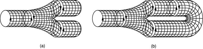
Figure 2: Both graphs are related to AdjQCD. The graph in (a) is a planar one; its Euler characteristic is $1$. The graph in (b) is a subleading one; it contains a loop and its Euler characteristic is $-1$.

At this point, we have developed all the tools we need to prove the orientifold planar equivalence. Let us see it with an example. Consider the first graph in figure 3. Apart from the combinatorial factor, its value is:

$$\mathcal{G}_{\textrm{Adj}}=\frac{1}{8}c_{1}c_{2}c_{3}\left<\mathrm{tr}U^{(E)}\,\mathcal{W}_{\textrm{Adj}}^{(1)}\,\mathcal{W}_{\textrm{Adj}}^{(2)\dagger}\,\mathcal{W}_{\textrm{Adj}}^{(3)\dagger}\,\mathcal{P}^{(E,1)}\,\mathcal{P}^{(1,2,3)}\,\mathcal{P}^{(2)}\,\mathcal{P}^{(3)}\right>_{c}$$ (10)

where $\left<\cdot\right>$ represents the integration with respect to the Haar measure. In the planar limit,

$$\mathcal{G}_{\textrm{Adj}}\simeq \frac{1}{8}c_{1}c_{2}c_{3}\left<\mathrm{tr}U^{(E)}\,\mathcal{P}^{(E,1)}\,\mathrm{tr}U^{(1)}\right>\;$$ (11)

$$\left<\mathrm{tr}U^{(1)\dagger}\,\mathrm{tr}U^{(2)\dagger}\,\mathrm{tr}U^{(3)\dagger}\,\mathcal{P}^{(1,2,3)}\right>\;\left<\mathrm{tr}U^{(2)}\,\mathcal{P}^{(2)}\right>\;\left<\mathrm{tr}U^{(3)}\,\mathcal{P}^{(3)}\right>\;.$$

Since the integration measure is invariant under the transformation $U\rightarrow U^{\dagger}$, the following equalities hold:

$$\left<\mathrm{tr}U^{(1)\dagger}\,\mathrm{tr}U^{(2)\dagger}\,\mathrm{tr}U^{(3)\dagger}\,\mathcal{P}^{(1,2,3)}\right>=\left<\mathrm{tr}U^{(1)}\,\mathrm{tr}U^{(2)}\,\mathrm{tr}U^{(3)}\,\mathcal{P}^{(1,2,3)\dagger}\right>$$

$$\mathcal{G}_{\textrm{Adj}}\simeq\frac{1}{8}iJc_{1}c_{2}c_{3}\left<\mathrm{tr}U^{(E)}\,\mathcal{P}^{(E,1)}\,\mathrm{tr}U^{(1)}\right>$$

$$\qquad\left<\mathrm{tr}U^{(1)}\,\mathrm{tr}U^{(2)}\,\mathrm{tr}U^{(3)}\,\mathcal{P}^{(1,2,3)\dagger}\right>\;\left<\mathrm{tr}U^{(2)}\,\mathcal{P}^{(2)}\right>\;\left<\mathrm{tr}U^{(3)}\,\mathcal{P}^{(3)}\right>$$ (12)

the latter being equal to the planar limit of the following graph (represented in the right side of figure 3) in AsQCD:

$$\mathcal{G}_{\textrm{As}}=c_{1}c_{2}c_{3}\left<\mathrm{tr}U^{(E)}\,\mathcal{W}_{\textrm{As}}^{(1)}\,\mathcal{W}_{\textrm{As}}^{(2)}\,\mathcal{W}_{\textrm{As}}^{(3)}\,\mathcal{P}^{(E,1)}\,\mathcal{P}^{(1,2,3)\dagger}\,\mathcal{P}^{(2)}\,\mathcal{P}^{(3)}\right>_{c}\;.$$ (13)

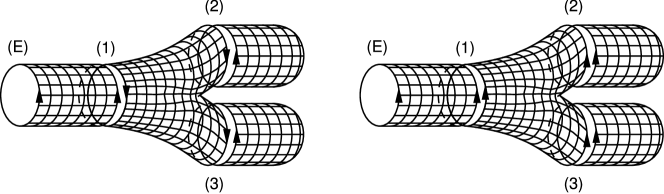
Figure 3: On the left, a graph of the expectation value of a WIlson loop for AdjQCD. On the right, a similar graph for AsQCD. The latter can be obtained from the former, simply by reversing all the directions of the link variables in the central connected component. The labels in the graphs refer to the Wilson loops.

This mechanism does not work with subleading graphs. It is enough to see the graph in the figure 2b to realize that no connected component can be consistently reversed to get a graph of AsQCD.

This result has a general validity. Since the integration measure is invariant under the substitution $U\rightarrow U^{\dagger}$, one can reverse all the directions in a connected component, without changing the value of the graph. Since planar graphs do not contain loops, one can independently choose which connected components to reverse. Reversing the directions of some components is equivalent to interchanging $\mathcal{W}_{\textbf{As}}\leftrightarrow\frac{1}{2}\mathcal{W}_{\textbf{Adj}}$. In this way, one can change the representation of the fermion and interchange Dirac with Majorana fermion. No change in the coefficients $c(\alpha)$ is needed, because they are representation-independent. In conclusion, planar equivalence comes from the graph-by-graph equality of expectation values of the two theories.

4 Conclusions

The results obtained are based on the possibility of expanding the expectation values as power series in $\lambda^{-1}$ and $\kappa$. Of course, a phase transition can exist in the plane $(\lambda,\kappa)$. Thus, the present work proves the orientifold planar equivalence only in the phase containing the point $\lambda=\infty$ and $\kappa=0$.

It is known that pure $SU(N)$ gauge theory in two dimensions on the lattice has a phase transition in the planar limit (also at a finite volume) between a strong-coupling and a weak-coupling phase [12]. Moreover, Kiskis, Narayanan and Neuberger [13, 14] showed numerically that such a phase transition exists in four dimensions, too.

At the moment, the phase structure of gauge theories with fermions in a two-indices representation is not known.

Clearly, it is also conceivable that the strong-coupling and large-mass phase does not contain the continuum limit (that is at $\lambda=0$ and $\kappa=\infty$). In this case, no information can be inferred on the validity of the orientifold planar equivalence between the two theories on the continuum.

References

- [1] A. Armoni, M. Shifman and G. Veneziano, Nucl. Phys. B 667, 170 (2003) [arXiv:hep-th/0302163].
- [2] A. Armoni, M. Shifman and G. Veneziano, Phys. Rev. Lett. 91, 191601 (2003) [arXiv:hep-th/0307097].
- [3] A. Armoni, M. Shifman and G. Veneziano, arXiv:hep-th/0403071.
- [4] A. Armoni, M. Shifman and G. Veneziano, Phys. Lett. B 579, 384 (2004) [arXiv:hep-th/0309013].
- [5] T. DeGrand, R. Hoffmann, S. Schaefer and Z. Liu, Phys. Rev. D 74, 054501 (2006) [arXiv:hep-th/0605147].
- [6] A. Armoni, M. Shifman and G. Veneziano, Phys. Rev. D 71, 045015 (2005) [arXiv:hep-th/0412203].
- [7] M. Unsal and L. G. Yaffe, arXiv:hep-th/0608180.
- [8] A. Patella, Phys. Rev. D 74, 034506 (2006) [arXiv:hep-lat/0511037].
- [9] H. J. Rothe, “Lattice gauge theories: An introduction”, World Scientific.
- [10] B. Collins and P. Sniady, arXiv:math-ph/0402073.
- [11] G. ’t Hooft, arXiv:hep-th/0204069.
- [12] D. J. Gross and E. Witten, Phys. Rev. D 21, 446 (1980).
- [13] J. Kiskis, R. Narayanan and H. Neuberger, Phys. Lett. B 574, 65 (2003) [arXiv:hep-lat/0308033].
- [14] R. Narayanan and H. Neuberger, PoS LAT2005, 005 (2006) [arXiv:hep-lat/0509014].