Heavy baryon mass spectrum from lattice QCD with 2+1 flavors

Abstract:

We study the heavy baryon mass spectrum on gauge configurations that include 2+1 flavors of dynamical improved staggered quarks. A valence clover heavy quark is combined with two improved staggered light quark propagators to form baryons with different flavors. We are using MILC coarse gauge configurations with a lattice spacing of about 0.12 fm. In this preliminary investigation, we explore the chiral limit by studying two light sea quark masses, three different strange valence quark masses, and nine different light valence quark masses ranging from 0.1 to 0.4 times the nominal strange quark mass.

1 Introduction

Heavy baryons have been extensively investigated by experimental and theoretical approaches. From experiment, the singly charmed heavy baryon mass spectrum is well known; however, the other heavy baryon masses are only crudely known. From lattice QCD, there are several quenched calculations for the heavy baryon mass spectrum [1–6], and most results are in fair agreement with observed values. In this project, we apply lattice QCD with dynamical sea quarks for the same objective. In the future, we hope to study semi-leptonic decays of heavy baryons [7] [4].

We present preliminary results for the mass spectrum of five different singly charmed heavy $\frac{1}{2}^{+}$ baryons: $\Lambda_{c}$, $\Sigma_{c}$, $\Xi_{c}$, $\Xi_{c}^{\prime}$, and $\Omega_{c}$. In this work, we use two different interpolating operators studied in Ref. [1] and construct two-point functions using the method of Wingate et al. [8] to combine staggered propagators for the light valence quarks and a Wilson type (clover) propagator for the heavy valence quark.

2 Construction of two-point functions

The interpolating operators to describe $\frac{1}{2}^{+}$ singly heavy baryons are [1]

$$\mathcal{O}_{5}=\epsilon_{abc}(\psi_{1}^{aT}C\gamma_{5}\psi_{2}^{b})\Psi_{H}^{c},\;\;\;\;\;\;\;\mathcal{O}_{\mu}=\epsilon_{abc}(\psi_{1}^{aT}C\gamma_{\mu}\psi_{2}^{b})\Psi_{H}^{c},$$ (1)

where $\epsilon_{abc}$ is the Levi-Civita tensor, $\psi_{1}$ and $\psi_{2}$ are light valence quark fields for up, down, or strange quarks, $\Psi_{H}$ is the heavy valence quark field, and $C$ is the charge conjugation matrix. As can be seen, the spinor indices of the light quark fields are contracted together, so the spinor index of the operator comes from $\Psi_{H}$. Basically, $\mathcal{O}_{5}$ is the operator for $s^{\pi}=0^{+}$, and $\mathcal{O}_{\mu}$ is for $s^{\pi}=1^{+}$, where $s^{\pi}$ is spin parity state for light quark pair. Each heavy baryon is obtained by choosing different quark flavor combinations, shown in Table 1.

Baryon	Content	Operator	$J^{p}$	$s^{\pi}$
$\Lambda_{c}$	$llc$	$\mathcal{O}_{5}$		$0^{+}$
$\Xi_{c}$	$lsc$	$\mathcal{O}_{5}$		$0^{+}$
$\Sigma_{c}$	$llc$	$\mathcal{O}_{\mu}$	$\frac{1}{2}^{+}$	$1^{+}$
$\Xi_{c}^{\prime}$	$lsc$	$\mathcal{O}_{\mu}$		$1^{+}$
$\Omega_{c}$	$ssc$	$\mathcal{O}_{\mu}$		$1^{+}$

Table 1: Heavy baryons, flavor contents and operators. $J^{p}$ is total spin parity of the heavy baryon, and $s^{\pi}$ is spin parity of the light quark pair. In the quark content column, $l$ is the light valence quark, $s$ is the strange quark, and $c$ is the charm quark.

Since we use staggered fermion propagators for the light quarks, and a Wilson type propagator for the heavy quark, we will use the method of Wingate et al. [8] to convert from a staggered propagator to a naive quark propagator. They show

$$G_{\psi}(x,y)=\Omega(x)\Omega^{\dagger}(y)G_{\chi}(x,y)$$ (2)

where,

$$\Omega(x)=\prod_{\mu}(\gamma_{\mu})^{x_{\mu}/a}.$$ (3)

$G_{\psi}(x,y)$ is the naive quark propagator, and $G_{\chi}(x,y)$ is the staggered quark propagator. With this basic relationship, we can construct the heavy baryon two-point functions

$$C_{\alpha\beta}(\vec{p},t) = \sum_{\vec{x}}e^{-i\vec{p}\cdot\vec{x}}\langle\mathcal{O}_{5\alpha}(\vec{x},t)\overline{\mathcal{O}}_{5\beta}(\vec{0},0)\rangle$$ (4)

$$= \sum_{\vec{x}}e^{-i\vec{p}\cdot\vec{x}}\epsilon_{abc}\epsilon_{a^{\prime}b^{\prime}c^{\prime}}\mathbf{tr}[G_{1}^{aa^{\prime}T}(x,0)C\gamma_{5}G_{2}^{bb^{\prime}}(x,0)C\gamma_{5}]G_{H\alpha\beta}^{cc^{\prime}}(x,0).$$ (5)

$G_{1}(x,0)$ and $G_{2}(x,0)$ are naive light quark propagators, $G_{H}(x,0)$ is the heavy quark propagator, and $\alpha$ and $\beta$ are spinor indices. As expected from the property of the interpolating operator, the spinor structure of the heavy baryon is determined from the heavy quark. Note that the trace in Eq. 5 is for spinor indices, not for color indices. Now, using Eq. 2,

$$G_{2}^{bb^{\prime}}(x,0)=\Omega(x)\Omega^{\dagger}(0)G_{2\chi}^{bb^{\prime}}(x,0)=\Omega(x)G_{2\chi}^{bb^{\prime}}(x,0)$$ (6)

and

$$G_{1}^{aa^{\prime}T}(x,0)=\Omega^{T}(x)G_{1\chi}^{aa^{\prime}}(x,0).$$ (7)

So

$$C_{\alpha\beta}(\vec{p},t)=\sum_{\vec{x}}e^{-i\vec{p}\cdot\vec{x}}\epsilon_{abc}\epsilon_{a^{\prime}b^{\prime}c^{\prime}}\mathbf{tr}[\Omega^{T}(x)C\gamma_{5}\Omega(x)C\gamma_{5}]G_{1\chi}^{aa^{\prime}}(x,0)G_{2\chi}^{bb^{\prime}}(x,0)G_{H\alpha\beta}^{cc^{\prime}}(x,0).$$ (8)

But the trace can be simplified:

$$\mathbf{tr}[\Omega^{T}(x)C\gamma_{5}\Omega(x)C\gamma_{5}]=\mathbf{tr}[-1(-1)^{x_{1}+x_{3}}(-1)^{x_{1}+x_{3}}]=-4.$$ (9)

Finally, the two-point function can be expressed as,

$$C_{\alpha\beta}(\vec{p},t)=\sum_{\vec{x}}e^{-i\vec{p}\cdot\vec{x}}\epsilon_{abc}\epsilon_{a^{\prime}b^{\prime}c^{\prime}}(-4)G_{1\chi}^{aa^{\prime}}(x,0)G_{2\chi}^{bb^{\prime}}(x,0)G_{H\alpha\beta}^{cc^{\prime}}(x,0).$$ (10)

This two-point function is constructed using the operator $\mathcal{O}_{5}$. Similarly, we can derive the two-point function with the other operator $\mathcal{O}_{\mu}$.

3 Data analysis

We use two ensembles of $20^{3}\times 64$ MILC coarse dynamical lattice gauge configurations with lattice spacing $a\approx 0.12$ fm. We investigate 385 configurations for the ensemble with $am_{l}=0.01$, and $am_{s}=0.05$, and 458 configurations for the ensemble with $am_{l}=0.02$, and $am_{s}=0.05$, where $m_{l}$ is the light sea quark mass, and $m_{s}$ is the strange sea quark mass. For each configuration, we require several propagators for the valence quarks. We compute nine different staggered light quark propagators with masses between 0.005 and 0.02, and three staggered strange quark propagators with masses 0.024, 0.03, and 0.0415. For the heavy charm quark, we use only one kappa value $\kappa=0.122$ based on tuning for our heavy-light meson decay constant calculation [9].

For fitting the baryon propagators, we use correlated least squares fits, and for error estimation, we generate 1000 bootstrap samples. Taking into account the periodic boundary condition in time for the valence quarks and the staggered phases, the fit model is

$$P(t)= Ae^{-mt}+Ae^{-m(T-t)}+(-1)^{t}\tilde{A}e^{-\tilde{m}t}+(-1)^{t}\tilde{A}e^{-\tilde{m}(T-t)}$$

$$+A_{*}e^{-m_{*}t}+A_{*}e^{-m_{*}(T-t)}+(-1)^{t}\tilde{A}_{*}e^{-\tilde{m}_{*}t}+(-1)^{t}\tilde{A}_{*}e^{-\tilde{m}_{*}(T-t)},$$ (11)

where $m$ is the ground state of positive parity, $\tilde{m}$ has opposite parity, and the values with an asterisk denote the corresponding excited states. In practice, most propagators could be fit including contributions with just two or three particles. In most cases the confidence level of the fit is between 40 and 60 percent. (Of course, on each ensemble, baryon propagators with different valence masses are correlated.)

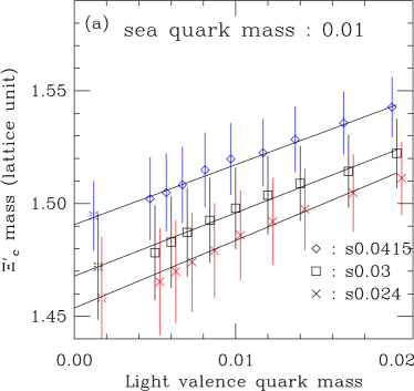
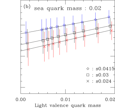
Figure 1: Chiral extrapolation of light valence quark mass on each ensemble.

To discuss extrapolation to the chiral limit, we present an example for $\Xi_{c}^{\prime}$. First, let’s look at the extrapolation of the light valence quark mass shown in Fig. 1. As we can see, there are three sets of data for each ensemble corresponding to each valence strange quark mass. We have performed linear extrapolations although there is a very small curvature seen for the lighter sea quark mass (Fig. 1(a)). The bursts show the linear extrapolation to the bare light quark mass 0.00148 [10] in lattice units on this ensemble. Next, we interpolate in the strange quark mass (Fig. 2(a)) and extrapolate in the light sea quark mass (Fig. 2(b)). The bare strange quark mass was estimated to be 0.039 [10]. In Fig. 2(a), we see that linear interpolation in the strange quark mass is perfectly adequate.

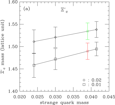
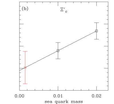
Figure 2: Interpolation of strange quark mass (a), and extrapolation of light sea quark mass (b). The bare strange quark mass is 0.039, and the bare light sea quark mass is 0.00148. Bursts are the interpolated and extrapolated results.

After extrapolation in the light sea quark mass, we find the mass of $\Xi_{c}^{\prime}$ within the partially quenched approximation. Alternatively, there is a full QCD point for each ensemble, and we can simultaneously extrapolate in light sea and valence masses. Fig. 3 compares the results of these two approaches for four baryons. As we can see, the full QCD results have smaller error bars than the partially quenched results. Our multistep partially quenched interpolation and extrapolation procedure may be causing larger errors than the simple full QCD extrapolation in light quark mass. If we had fit all the data with a partially quenched formula depending on both sea and valence quark masses, the partially quenched QCD chiral extrapolation might have given smaller error bars than the fit to the limited full QCD data. (We plan to try that in the future.) We present our preliminary results here based upon the full QCD extrapolation.

Figure 3: Full QCD compared with partially quenched QCD chiral extrapolation. Four different masses of singly heavy baryons. Note that $\Omega_{c}$ dose not appear, since $\Omega_{c}$ does not contain light valence quarks.

4 Results

Figure 4: Mass splitting (a), and mass spectrum (b) of five different singly charmed heavy baryons with $\frac{1}{2}^{+}$ in MeV units.

We present mass splittings in MeV between five different singly heavy baryons in Fig. 4(a). Square data points correspond to the experiment data [11], and crosses with error bars indicate our results. The experiment errors are considerably smaller than our own, so we ignore them here. Our results agree with the experimental values within errors. In fact, the agreement is so good, we wonder if we are overestimating our errors. On the other hand, all the baryon masses are correlated.

We also present the mass spectrum itself in Fig. 4(b). In order to get the physical mass $M_{phy}$ of a heavy baryon, we need to add a constant mass shift $\Delta$ to the calculated mass $M_{cal}$, i.e.

$$M_{phy}=M_{cal}+\Delta.$$ (12)

In this project, we chose the constant mass shift $\Delta$ in a simple way to best match the average of the experimental masses.

$$\Delta=Average(M_{exp}-M_{cal}).$$ (13)

We should investigate the momentum dependence of the heavy baryon energy in order to calculate the kinetic mass of the state. If we use the dispersion relation, we can take the kinetic mass $M_{kin}$ as the physical mass $M_{phy}$ [8],

$$M_{kin}=\frac{|\vec{p}|^{2}-[E(\vec{p})-E(0)]^{2}}{2[E(\vec{p})-E(0)]}.$$ (14)

5 Future study

We have presented preliminary spectrum results based on dynamical lattice QCD. The study can be extended in several ways. We shall investigate singly bottom baryons and doubly charmed baryons. Recently, the SELEX collaboration reported the measurement of the doubly charmed baryon $\Xi_{cc}^{+}$ [12], so it would be timely to compute the doubly charmed baryon spectrum. So far we have only studied $\frac{1}{2}^{+}$ states, and we would like to extend the study to $\frac{3}{2}^{+}$ states. In this way, we can investigate the hyperfine splitting problem [3] [5] in heavy baryons. In addition, we can increase statistics by using more configurations and ensembles, and additional time sources for our propagators. We also need to clarify the taste structure of our baryon operators.

- [1] K.C. Bowler et al. (UKQCD Collaboration), Phys. Rev. D 54 (1996) 3619.
- [2] N. Mathur et al., Phys. Rev. D 66 (2002) 014502.
- [3] R.M. Woloshyn, Phys. Lett. B 476 (2000) 309.
- [4] S. Gottlieb and S. Tamhankar, Nucl. Phys. Proc. Suppl. 119 (2003) 644.
- [5] A. Ali Khan et al., Phys. Rev. D 62 (2000) 054505.
- [6] T.W. Chiu and T.H. Hsieh, Nucl. Phys. A 755 (2005) 471c.
- [7] K.C. Bowler et al. (UKQCD Collaboration), Phys. Rev. D 57 (1998) 6948.
- [8] M. Wingate et al., Phys. Rev. D 67 (2003) 054505.
- [9] C. Aubin et al. (Fermilab Lattice, MILC, and HPQCD Collaborations), Phys. Rev. Lett. 95 (2005) 122002.
- [10] C. Aubin et al. (MILC Collaboration), Phys. Rev. D 70 (2004) 114501.
- [11] W.M. Yao et al., J. Phys. G 33 (2006) 1.
- [12] A. Ocherashvili et al., Phys. Lett. B 628 (2005) 18.