Nucleon structure in the chiral regime with domain wall fermions on an improved staggered sea

Abstract:

Moments of unpolarized, helicity, and transversity distributions, electromagnetic form factors, and generalized form factors of the nucleon are presented from a preliminary analysis of lattice results using pion masses down to 359 MeV. The twist two matrix elements are calculated using a mixed action of domain wall valence quarks and asqtad staggered sea quarks and are renormalized perturbatively. Several observables are extrapolated to the physical limit using chiral perturbation theory. Results are compared with experimental moments of quark distributions and electromagnetic form factors and phenomenologically determined generalized form factors, and the implications on the transverse structure and spin content of the nucleon are discussed.

1 Introduction

Our use of lattice field theory to calculate the structure of the nucleon from first principles has two complementary objectives. One goal is to achieve quantitative agreement with experimental observables such as nucleon form factors and parton distributions, to confirm the quantitative precision of our solution of QCD and to establish the credibility to make predictions and guide future experiments. However, merely producing a black box that only reproduces experiment would be unfulfilling. Hence, our second goal is to obtain insight into how QCD works, revealing, for example, the origin of the nucleon spin, physical mechanisms, such as instantons, responsible for essential features of hadron structure, and the dependence on parameters of QCD like $N_{C}$, $N_{f}$, $m_{q}$, and the gauge group. A crucial issue in making quantitative contact with experiment is calculating sufficiently far into the chiral regime that reliable chiral extrapolations to the physical pion mass are possible. Hence, in this work we have utilized the extensive set of configurations with dynamical improved staggered quarks generated by the MILC collaboration [1] to explore nucleon structure in the chiral regime.

2 Mixed Action Lattice Calculation

As explained in Ref. [2], we utilize a hybrid action combining domain wall valence fermions with improved staggered sea quarks. Improved staggered sea quarks offer the advantage that due to the relative economy of the algorithm, lattices with large volumes, small pion masses, and several lattice spacings are publicly available from the MILC collaboration. Although the fourth root of the fermion determinant remains controversial, current evidence suggests it is manageable [3, 4]. Renormalization group arguments indicate that the coefficient of the nonlocal term approaches zero in the continuum limit [5], partially quenched staggered chiral perturbation theory accounts well for the artificial properties at finite lattice spacing [6], and the action has the advantage of being improved to ${\cal{O}}(a^{2})$. Domain wall valence quarks offer equally compelling advantages to justify investing resources in calculating hadron observables on staggered configurations that are roughly comparable to the resources required to generate the configurations themselves. Domain wall fermions prevent mixing of quark observables by chiral symmetry, are accurate to ${\cal{O}}(a^{2})$, and possess a conserved five dimensional axial current that facilitates calculation of renormalization factors. In addition, hybrid action (often referred to as mixed action) chiral perturbation theory results are available for many observables, and by virtue of an exact lattice chiral symmetry, one loop results have the simple chiral behavior observed in the continuum. The parameters of the configurations used in this work are shown in Table [1], and details can be found in Refs. [2, 7].

$am_{u/d}^{\mathrm{asqtad}}$	$L/a$	$L$	$m_{\pi}^{\mathrm{DWF}}$	#
		$\mathrm{fm}$	$\mathrm{MeV}$
$0.05$	$20$	$2.52$	$761$	$425$
$0.04$	$"$	$"$	$693$	$350$
$0.03$	$"$	$"$	$594$	$564$
$0.02$	$"$	$"$	$498$	$486$
$0.01$	$"$	$"$	$354$	$656$
$0.01$	$28$	$3.53$	$353$	$270$

Table 1: Lattice parameters used in this work.

3 Moments of Parton Distributions

Parton distributions measure forward matrix elements of the gauge invariant light cone operators

$${\cal O}_{\Gamma}(x)=\int\!\frac{d\lambda}{4\pi}e^{i\lambda x}\overline{q}(-\lambda n/2)\Gamma\,{\cal P}e^{-ig\int_{\lambda/2}^{-\lambda/2}d\alpha\,n\cdot A(\alpha n)}\!q(\lambda n/2),$$ (1)

where $x$ is a momentum fraction, $n$ is a light cone vector and $\Gamma=/\!\!\!\!\!{n}$ or $\Gamma=/\!\!\!\!\!{n}\gamma_{5}$. Using the operator product expansion, the operators in Eq. [1] yield towers of symmetrized, traceless local operators that can be evaluated on a Euclidean lattice

$${\cal O}_{[\gamma_{5}]}^{\{\mu_{1}\ldots\mu_{n}\}}=\overline{q}\gamma^{\{\mu_{1}}[\gamma_{5}]i\stackrel{{\scriptstyle\leftrightarrow}}{{D}}{}^{\!\mu_{2}}\!\cdots i\stackrel{{\scriptstyle\leftrightarrow}}{{D}}{}^{\!\mu_{n}\}}q\,,$$ (2)

where $[\gamma_{5}]$ denotes the possible inclusion of $\gamma_{5}$, the curly brackets represent symmetrization over the indices $\mu_{i}$ and subtraction of traces, and $\stackrel{{\scriptstyle\leftrightarrow}}{{D}}=1/2(\stackrel{{\scriptstyle\rightarrow}}{{D}}-\stackrel{{\scriptstyle\leftarrow}}{{D}})$. A related operator for transversity distributions is

$${\cal O}_{\sigma}^{\mu\{\mu_{1}\ldots\mu_{n}\}}=\overline{q}\gamma_{5}\sigma^{\mu\{\mu_{1}}i\stackrel{{\scriptstyle\leftrightarrow}}{{D}}{}^{\!\mu_{2}}\!\cdots i\stackrel{{\scriptstyle\leftrightarrow}}{{D}}{}^{\!\mu_{n}\}}q\,.$$ (3)

Using the notation and normalization of Ref. [8], the forward matrix elements $\langle P,S|{\cal O}^{\{\mu_{1}\ldots\mu_{n+1}\}}|P,S\rangle$ yield moments of the unpolarized quark distribution:

$$\langle x^{n}\rangle_{q}=\int_{0}^{1}\!\!dx\,x^{n}[q(x)+(-1)^{n+1}\overline{q}(x)],$$ (4)

the forward matrix elements $\langle P,S|{\cal O}_{\gamma_{5}}^{\{\mu_{1}\ldots\mu_{n+1}\}}|P,S\rangle$ yield moments of the helicity distribution:

$$\langle x^{n}\rangle_{\Delta q}=\int_{0}^{1}\!\!dx\,x^{n}[\Delta q(x)+(-1)^{n}\Delta\overline{q}(x)],$$ (5)

and the forward matrix elements $\langle P,S|{\cal O}_{\sigma}^{\mu\{\mu_{1}\ldots\mu_{n+1}\}}|P,S\rangle$ yield moments of the transversity distribution:

$$\langle x^{n}\rangle_{\delta q}=\int_{0}^{1}\!\!dx\,x^{n}[\delta q(x)+(-1)^{n+1}\delta\overline{q}(x)].$$ (6)

In this work, we calculate only connected diagrams, and hence concentrate as much as possible on isovector quantities.

All quark bilinear operators in Eqs. [2] and [3] are renormalized as follows [9]. The axial current is renormalized exactly using the conserved five dimensional axial current. By virtue of the suppression of loop integrals by HYP smearing, the ratio of the one-loop perturbative renormalization factor for a general bilinear operator to the renormalization factor for the axial current is within a few percent of unity, suggesting adequate convergence at one-loop level. Hence the complete renormalization factor is written as the exact axial current renormalization factor times the ratio of the perturbative renormalization factor for the desired operator divided by the perturbative renormalization factor for the axial current.

3.1 Chiral Perturbation Theory

Ideally, we would like to perform high statistics calculations at pion masses below 350 MeV and extrapolate them in pion mass and volume using a chiral perturbation theory expansion of sufficiently high order to provide a quantitatively controlled approximation. In practice, our most convincing chiral extrapolation has been for $g_{A}$ using the finite volume results including $\Delta$ intermediate states of Ref. [10], where the fit involving 6 low energy parameters yielded an excellent fit up to the order of a 700 MeV pion mass and agreed with experiment with 6.8% errors [11]. Similar extrapolations of $g_{A}$ have been performed by other groups [12]. This success for $g_{A}$ is particularly relevant to the subsequent discussion of nucleon spin, because it involves the same operators $\langle 1\rangle_{q}$ as $\Delta\Sigma$. We note that because the nucleon and $\Delta$ should be included together at large $N_{c}$ [13] and indeed show large cancellations in the axial charge, we prefer to include the $\Delta$ as an explicit degree of freedom in the analysis.

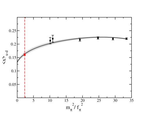
An unresolved puzzle in calculating moments of structure functions is the relatively flat behavior of the momentum fraction $\langle x\rangle$ at a constant value substantially higher than experiment [14, 15]. Hence, it is particularly interesting to ask whether a chiral perturbation theory fit determined without knowledge of the experimental result is in fact statistically consistent with experiment. Since there is presently insufficient data to perform a full analysis including the $\Delta$, here we present a simple self-consistent improved one-loop analysis using only nucleon degrees of freedom that appears to work very well in our regime.

The details will be presented in a future publication [16], but the basic idea is as follows. We begin with the one loop expression at scale $\mu$ [17, 18].

$$\langle x^{n}\rangle_{u-d}=a_{n}\left(1-\frac{(3g^{2}_{A,0}+1)}{(4\pi f_{\pi,\scriptscriptstyle{0}})^{2}}m_{\pi}^{2}\ln\left(\frac{m_{\pi}^{2}}{\mu^{2}}\right)\right)+b^{\prime}_{n}(\mu)m_{\pi}^{2}$$ (7)

in which we explicitly note that $g_{A,0}$ and $f_{\pi,\scriptscriptstyle{0}}$ are $g_{A}$ and $f_{\pi}$ in the chiral limit. We are free to choose the scale $\mu$ to be $f_{\pi}$. Additionally we replace $g_{A,0}$ and $f_{\pi,\scriptscriptstyle{0}}$ with their values at the given pion mass $g_{A,m_{\pi}}$ and $f_{\pi,m_{\pi}}$, so that the result may be rewritten as

$$\langle x^{n}\rangle_{u-d}=a_{n}\left(1-\frac{(3g_{A,m_{\pi}}^{2}+1)}{(4\pi)^{2}}\frac{m_{\pi}^{2}}{f_{\pi,m_{\pi}}^{2}}\ln\left(\frac{m_{\pi}^{2}}{f_{\pi,m_{\pi}}^{2}}\right)\right)+b_{n}\frac{m_{\pi}^{2}}{f_{\pi,m_{\pi}}^{2}}.$$ (8)

Figure 1: Zeroth moment of helicity distribution.

Figure 2: Zeroth moment of transversity distribution.

Figure 3: First moment of unpolarized distribution.

Figure 4: First moment of helicity distribution.

If we view this as an expansion in the ratio $r=\frac{m_{\pi}^{2}}{(4\pi)^{2}f^{2}_{\pi,m_{\pi}}}$, one can show that shifting to an expansion around $g_{A}$ and $f_{\pi}$ defined at another mass only introduces changes of ${\cal{O}}(r^{2})$. Hence, to leading order, we may write an expression in which we use the values $g_{A,lat}$, $f_{\pi,lat}$, and $m_{\pi,lat}$ calculated on the lattice at specific values of the quark mass. Then, the expressions for the moments of the unpolarized, helicity, and transversity distributions are the following:

$$\langle x^{n}\rangle_{u-d} = a_{n}\left(1-\frac{(3g_{A,\mathrm{lat}}^{2}+1)}{(4\pi)^{2}}\frac{m_{\pi,\mathrm{lat}}^{2}}{f_{\pi,\mathrm{lat}}^{2}}\ln\left(\frac{m_{\pi,\mathrm{lat}}^{2}}{f_{\pi,\mathrm{lat}}^{2}}\right)\right)+b_{n}\frac{m_{\pi,\mathrm{lat}}^{2}}{f_{\pi,\mathrm{lat}}^{2}}$$ (9)

$$\langle x^{n}\rangle_{\Delta u-\Delta d} = \Delta a_{n}\left(1-\frac{(2g_{A,\mathrm{lat}}^{2}+1)}{(4\pi)^{2}}\frac{m_{\pi,\mathrm{lat}}^{2}}{f_{\pi,\mathrm{lat}}^{2}}\ln\left(\frac{m_{\pi,\mathrm{lat}}^{2}}{f_{\pi,\mathrm{lat}}^{2}}\right)\right)+\Delta b_{n}\frac{m_{\pi,\mathrm{lat}}^{2}}{f_{\pi,\mathrm{lat}}^{2}}$$ (10)

$$\langle x^{n}\rangle_{\delta u-\delta d} = \delta a_{n}\left(1-\frac{(4g_{A,\mathrm{lat}}^{2}+1)}{2(4\pi)^{2}}\frac{m_{\pi,\mathrm{lat}}^{2}}{f_{\pi,\mathrm{lat}}^{2}}\ln\left(\frac{m_{\pi,\mathrm{lat}}^{2}}{f_{\pi,\mathrm{lat}}^{2}}\right)\right)+\delta b_{n}\frac{m_{\pi,\mathrm{lat}}^{2}}{f_{\pi,\mathrm{lat}}^{2}}\,.$$ (11)

These results allow a least-squares two-parameter fit to the lattice data for moments and provides an extrapolation to the physical pion mass with a corresponding error band. Note that the series is substantially rearranged, by virtue that the calculated values of $g_{A}$, $f_{\pi}$, and $m_{\pi}$ are used at each value of the bare quark mass. Although we cannot prove that this self-consistent improved one-loop result should be accurate throughout the range of our data, to the extent to which it is successful, we believe its success arises from this self-consistent rearrangement. Additionally, the use of physical rather than chiral limit values for $f_{\pi}$ was first tried in [19] and has since been studied in chiral perturbation [20, 21] and applied to a variety of lattice calculations [22, 23, 24, 25, 26].

3.2 Lattice Results

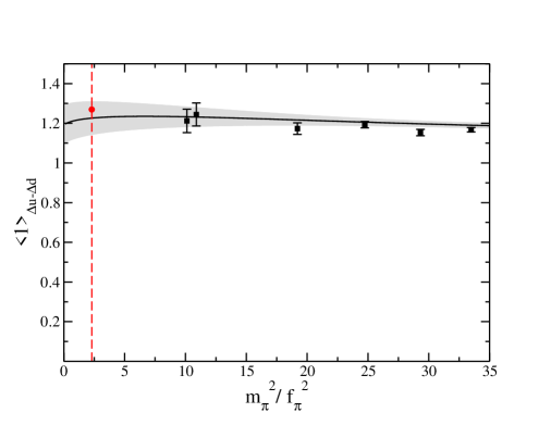
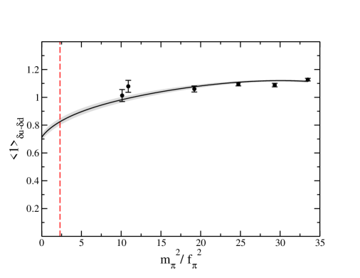
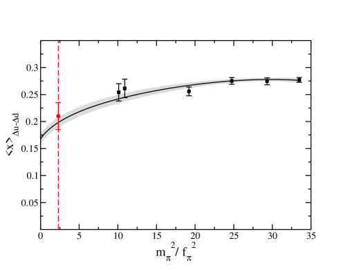
Here we show the results of this one-loop analysis. Figure [2] shows the result for $g_{A}$, which is nearly as good as the complete analysis of Ref. [11], and yields a comparable extrapolation and error bar. Reassured by this result, we show analogous results for $\langle 1\rangle_{\delta u-\delta d}$, $\langle x\rangle_{u-d}$, $\langle x\rangle_{\Delta u-\Delta d}$,$\langle x\rangle_{\delta u-\delta d}$, and $\langle x^{2}\rangle_{\delta u-\delta d}$ in Figs. [4]-[6].

Figure 5: First moment of transversity distribution.

Figure 6: Second moment of helicity distribution.

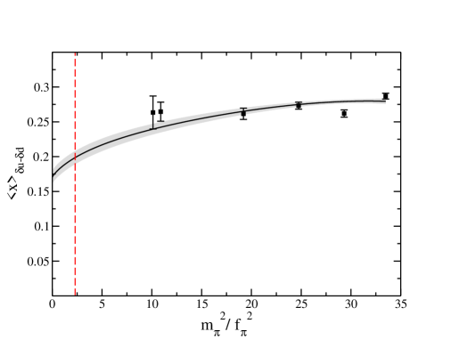
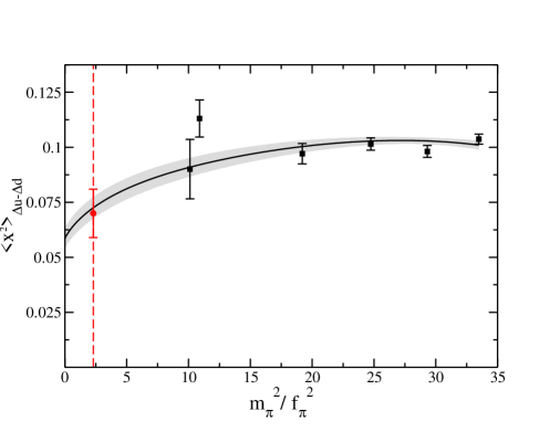
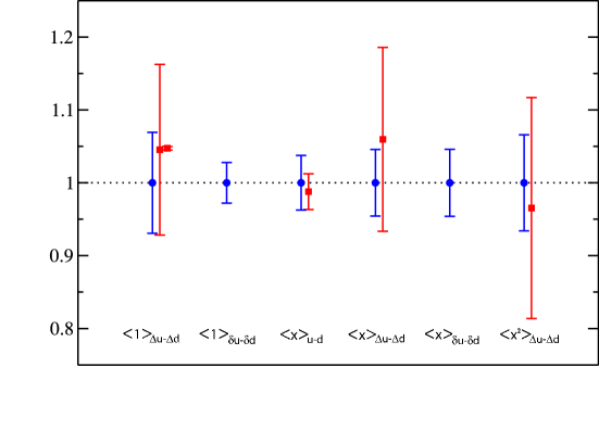
Note that in every case for which there is experimental data, this analysis, which in no way includes the experimental result in the fit, yields an extrapolation consistent with experiment. The results are collected together in Fig. [7], where because experimental results are not available for all cases, we have normalized all results to the corresponding lattice result.

Figure 7: The six moments considered in this work. Lattice results are shown in blue and experimental measurements in red, and each is normalized to the corresponding lattice result.

4 Form Factors

Form factors are interesting physically because at low momentum transfer they characterize the spatial size of charge and current distributions and at high momentum transfer they measure the ability of the nucleon to absorb a large momentum and distribute it to all the constituents such that the system remains in its ground state. Although for a relativistic system, the slope of the form factor is not precisely related to the rms radius, we will adhere to the common usage and refer to the slope as the rms radius. (We note in passing that the slope of $F_{1}$ is in fact related to the transverse rms radius in the infinite momentum frame.) Our primary focus here is on the qualitative approach to experiment as the quark mass is decreased, and to avoid uncalculated contributions of disconnected diagrams, we consider isovector form factors.

The nucleon vector current form factors $F_{1}$ and $F_{2}$ are defined by

$$\langle p|\overline{\psi}\gamma^{\mu}\psi|p^{\prime}\rangle=\overline{u}(p)[F_{1}(q^{2})\gamma^{\mu}+F_{2}(q^{2})\frac{i\sigma^{\mu\nu}q_{\nu}}{2m}]u(p^{\prime})\,.$$ (12)

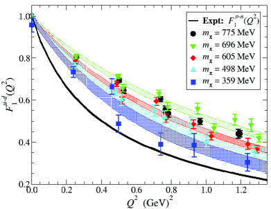
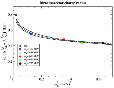
Figure [9] shows the lattice data and dipole fits for $F_{1}$ at five pion masses, and one observes that the lattice results systematically approach the experimental curve as the pion mass decreases to 359 MeV. One can quantitatively observe how the rms radius $\langle r^{2}\rangle^{n-p}$ defined from the slope approaches the experimental value by fitting it with the simple chiral extrapolation formula [27]

$$\langle r^{2}\rangle^{u-d}=a_{0}-\frac{1+5g_{A}^{2}}{(4\pi f_{\pi})^{2}}\log\left(\frac{m^{2}_{\pi}}{m^{2}_{\pi}+\Lambda^{2}}\right),$$ (13)

where $\Lambda$ is a phenomenological cutoff or equivalently, coefficient of an $m_{\pi}^{2}$ term in the expansion. Note that, in contrast to most chiral extrapolations which contain finite terms of the form $m_{\pi}^{2}\log m_{\pi}^{2}$, the isovector radius diverges like $\log m_{\pi}^{2}$, rendering the variation of the radius quite substantial near the physical pion mass. Figure [9] shows the results of fitting the lattice data with Eq. [13], and one notes that without having been constrained to do so, the chiral extrapolation is consistent with experiment.

Figure 8: F₁ isovector form factor at five masses compared with experiment [28].

Figure 9: Chiral extrapolation of isovector form factor slope.

Figure 10: Isovector form factor ratio $F_{2}/F_{1}$ at three masses compared with experiment [28].

Figure 11: Isovector form factor ratio $G_{A}/F_{1}$ at four masses compared with experiment.

Figure 12: Isovector form factor ratio $G_{P}/G_{A}$ at six masses compared with experiment.

Figure 13: Isovector pion pole contribution, normalized as $(q^{2}+m_{\pi}^{2})G_{P}/4m^{2}G_{A}$, at $m_{\pi}=$350 MeV .

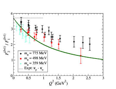
The form factor $F_{2}$ is of particular interest following the observation at JLab [29] that measurement of spin transfer yields a form factor that decreases more slowly with momentum transfer than the traditional Rosenbluth separation, which is now believed to suffer from substantial contamination from two photon exchange contributions. Figure [11] shows that the lattice results indeed approach the experimental ratio $F_{2}/F_{1}$ from spin transfer as the pion mass decreases.

The nucleon axial vector current form factors $G_{A}$ and $G_{P}$ are defined by

$$\langle p|\overline{\psi}\gamma^{\mu}\gamma_{5}\psi|p^{\prime}\rangle=\overline{u}(p)[G_{A}(q^{2})\gamma^{\mu}\gamma_{5}+\frac{q^{\mu}}{2m}\gamma_{5}G_{P}(q^{2})+\sigma^{\mu\nu}\gamma_{5}q_{\nu}G_{M}(q^{2})]u(p^{\prime}).$$ (14)

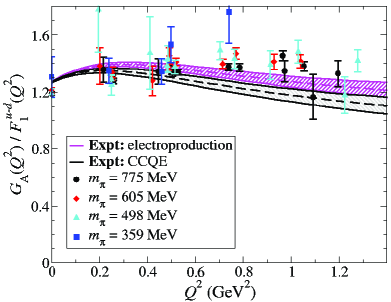
Figure [11] shows lattice calculations of the isovector ratio $G_{A}/F_{1}$ compared with experimental form factors extracted from pion photoproduction and neutrino scattering. Again, to within the roughly 10% discrepancy between the two experiments, the lattice results are qualitatively consistent with experiment. In the soft pion limit, $G_{P}$ is dominated by the pion pole:

$$G_{p}(q^{2})\sim\frac{4m^{2}G_{A}(q^{2})}{q^{2}+m^{2}_{\pi}}.$$ (15)

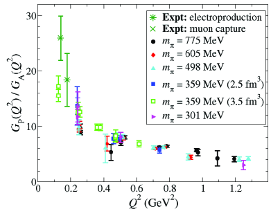
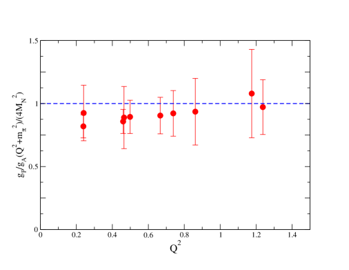
Figure [13] shows lattice results for the the ratio $G_{P}/G_{A}$ compared with experiment. To demonstrate the degree to which Eq. [15] is satisfied, Fig. [13] shows the ratio $(q^{2}+m_{\pi}^{2})G_{P}/4m^{2}G_{A}$ for lattice data at pion mass 350 MeV, which is consistent with unity.

5 Generalized Parton Distributions

Figure 14: Generalized form factors $A_{20},B_{20}$ and $C_{20}$ for $u-d$ and $u+d$ at four masses.

Off diagonal matrix elements of the tower of operators in Eq. [2] yield the generalized form factors

$$\langle P^{\prime}|{\cal O}^{\mu_{1}}|P\rangle = \langle\!\langle\gamma^{\mu_{1}}\rangle\!\rangle A_{10}(t)+\frac{\mbox{i}}{2m}\langle\!\langle\sigma^{\mu_{1}\alpha}\rangle\!\rangle\Delta_{\alpha}B_{10}(t)\,,$$

$$\langle P^{\prime}|{\cal O}^{\{\mu_{1}\mu_{2}\}}|P\rangle = \overline{P}{}^{\{\mu_{1}}\langle\!\langle\gamma^{\mu_{2}\}}\rangle\!\rangle A_{20}(t)+\frac{\mbox{i}}{2m}\overline{P}{}^{\{\mu_{1}}\langle\!\langle\sigma^{\mu_{2}\}\alpha}\rangle\!\rangle\Delta_{\alpha}B_{20}(t)+\frac{1}{m}\Delta^{\{\mu_{1}}\Delta^{\mu_{2}\}}C_{20}(t)\,,$$

$$\langle P^{\prime}|{\cal O}^{\{\mu_{1}\mu_{2}\mu_{3}\}}|P\rangle = \overline{P}{}^{\{\mu_{1}}\overline{P}{}^{\mu_{2}}\langle\!\langle\gamma^{\mu_{3}\}}\rangle\!\rangle A_{30}(t)+\frac{\mbox{i}}{2m}\overline{P}{}^{\{\mu_{1}}\overline{P}{}^{\mu_{2}}\langle\!\langle\sigma^{\mu_{3}\}\alpha}\rangle\!\rangle\Delta_{\alpha}B_{30}(t)$$ (16)

$$+ \Delta^{\{\mu_{1}}\Delta^{\mu_{2}}\langle\!\langle\gamma^{\mu_{3}\}}\rangle\!\rangle A_{32}(t)+\frac{\mbox{i}}{2m}\Delta^{\{\mu_{1}}\Delta^{\mu_{2}}\langle\!\langle\sigma^{\mu_{3}\}\alpha}\rangle\!\rangle\Delta_{\alpha}B_{32}(t),$$

where we use the short-hand notation $\langle\!\langle\Gamma\rangle\!\rangle=\overline{U}(P^{\prime},\Lambda^{\prime})\Gamma U(P,\Lambda)$ for matrix elements of Dirac spinors $U$ and where $\Delta=P^{\prime}-P$ and $t=\Delta^{2}$.

Of particular interest in this work is the relationship between the generalized form factors and the origin of the nucleon spin. The contribution of the spin of the up and down quarks to the total spin of the nucleon is given by the zeroth moment of the spin dependent structure function $\langle 1\rangle_{\Delta q}$ as

$$\frac{1}{2}\Delta\Sigma=\frac{1}{2}\langle 1\rangle_{\Delta u+\Delta d}\,.$$ (17)

Note both that our previous calculation of $g_{A}$ confirms our ability to calculate the connected contributions to $\langle 1\rangle_{\Delta q}$ accurately on the lattice and that $\Delta\Sigma$ requires the calculation of disconnected as well as connected contributions. Throughout this section, we will only discuss the results of connected diagrams, so all results will eventually need to be corrected for the effect of disconnected diagrams as well.

The total contribution to the nucleon spin from both the spin and orbital angular momentum of quarks is given by the Ji sum rule [30]:

$$J_{q}=\frac{1}{2}\left(A_{20}^{u+d}(0)+B_{20}^{u+d}(0)\right),$$ (18)

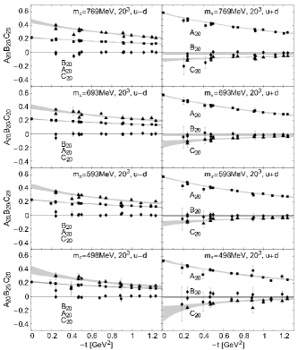
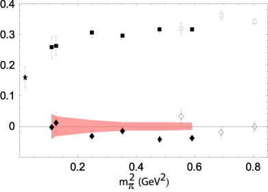
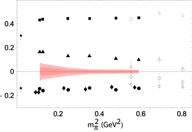
so that the contribution of the orbital angular momentum is given by $L_{q}=J_{q}-\frac{1}{2}\Delta\Sigma$. Earlier calculations in the heavy quark regime showed that for 700 MeV pions, roughly 68% of the spin of the nucleon arises from the spin of quarks, 0% arises from orbital angular momentum, and hence the remaining 32% must come from gluons [31, 32, 33]. Figure [14] shows the recent lattice data for $A_{20}$, $B_{20}$ and $C_{20}$ for lighter pion masses, and the results for $\Delta\Sigma$ and $L_{q}$ are shown in Fig. [16]. The full decomposition showing the contribution of spin and orbital angular momentum from up and down quarks is shown in Fig. [16]. Here, one observes that the angular momentum contributions of both up and down quark are separately substantial, and it is only the sum that is extremely small.

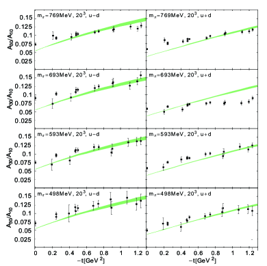
In previous work in the heavy quark regime [34], we have emphasized the dramatic differences in the slopes of $A_{10}$, $A_{20}$, and $A_{30}$ and the fact that this reflects a sharp decrease in the transverse size of the nucleon as $x$ approaches 1. To show that this behavior also arises in the chiral regime, Fig. [17] shows that the slope of the form factor ratio $A_{30}/A_{10}$ differs substantially from unity as the pion mass is decreased and also approaches the result given by a phenomenological parameterization of the generalized parton distributions [35].

Figure 15: Nucleon spin decomposition. Squares denote $\Delta\Sigma^{u+d}/2$, the star indicates the experimental quark spin contribution, and diamonds denote $L^{u+d}$.

Figure 16: Nucleon spin decomposition by flavor. Squares denote $\Delta\Sigma^{u}/2$, diamonds denote $\Delta\Sigma^{d}/2$, triangles denote $L^{u}$, and circles denote $L^{d}$.

Figure 17: Comparison of the ratio $A_{30}/A_{10}$ for $u-d$ and $u+d$ at four masses with a phenomenological fit to generalized parton distributions.

6 Conclusions

In summary, the hybrid combination of valence domain wall quarks on an improved staggered sea has enabled us to begin to enter the era of quantitative solution of full lattice QCD in the chiral regime. The axial charge, $g_{A}$, represents a successful, “gold-plated” test, which argues well for the prospects of quantitative control of a range of important nucleon observables. The chiral extrapolation of moments of quark distributions using our self-consistently improved one-loop analysis is encouraging, but of course we would still like to directly calculate the turn over in the approach to the chiral regime. Similarly, the general agreement between nucleon form factors of the vector and axial currents is highly encouraging. Generalized form factors are also being calculated well into the chiral regime, and give promise for understanding the origin of the nucleon spin and the transverse structure of the nucleon. In the long term, since lattice calculations determine moments of generalized parton distributions and experiments measure convolutions of generalized parton distributions, there is an excellent opportunity for synergy between experiment and theory in jointly determining generalized parton distributions. The final analysis of all the data shown in this work is currently being completed, and full results will be published in the near future.

This work also indicates obvious challenges for the future. Clearly the calculations must be extended to lower quark masses and finer lattices and analyzed with partially quenched hybrid chiral perturbation theory, and disconnected diagrams must be calculated. In addition, it is important to develop new techniques to explore form factors at high momentum transfer, gluon observables, and transition form factors for unstable states.

7 Acknowledgments

This work was supported by the DOE Office of Nuclear Physics under contracts DE-FC02-94ER40818, DE-AC05-06OR23177 and DE-AC05-84150, the EU Integrated Infrastructure Initiative Hadron Physics (I3HP) under contract RII3-CT-2004-506078, the DFG under contract FOR 465 (Forschergruppe Gitter-Hadronen-Phänomenologie) and the DFG Emmy-Noether program. Computations were performed on clusters at Jefferson Laboratory and at ORNL using time awarded under the SciDAC initiative. We are indebted to the members of the MILC collaboration for providing the dynamical quark configurations which made our full QCD calculations possible.

References

- [1] C. W. Bernard et al. Phys. Rev., D64:054506, 2001.
- [2] D. B. Renner et al. Nucl. Phys. Proc. Suppl., 140:255–260, 2005.
- [3] C. Bernard, M. Golterman, and Y. Shamir. Phys. Rev., D73:114511, 2006.
- [4] S. R. Sharpe. hep-lat/0610094, 2006.
- [5] Y. Shamir. hep-lat/0607007, 2006.
- [6] C. Bernard. Phys. Rev., D73:114503, 2006.
- [7] R. G. Edwards et al. PoS, LAT2005:056, 2006.
- [8] D. Dolgov et al. Phys. Rev., D66:034506, 2002.
- [9] B. Bistrovic et al. In preparation, 2006.
- [10] S. R. Beane and M. J. Savage. Phys. Rev., D70:074029, 2004.
- [11] R. G. Edwards et al. Phys. Rev. Lett., 96:052001, 2006.
- [12] A. Ali Khan et al. hep-lat/0603028, 2006.
- [13] R. F. Dashen, E. Jenkins, and A. V. Manohar. Phys. Rev., D49:4713–4738, 1994.
- [14] W. Detmold et al. Phys. Rev. Lett., 87:172001, 2001.
- [15] K. Orginos, T. Blum, and S. Ohta. Phys. Rev., D73:094503, 2006.
- [16] D. B. Renner et al. In preparation, 2006.
- [17] D. Arndt and M. J. Savage. Nucl. Phys., A697:429–439, 2002.
- [18] J. W. Chen and X. D. Ji. Phys. Lett., B523:107–110, 2001.
- [19] S. R. Beane, P. F. Bedaque, K. Orginos, and M. J. Savage. Phys. Rev., D73:054503, 2006.
- [20] J. W. Chen, D. O’Connell, R. S. Van de Water, and A. Walker-Loud. Phys. Rev., D73:074510, 2006.
- [21] D. O’Connell. hep-lat/0609046, 2006.
- [22] S. R. Beane et al. hep-lat/0607036, 2006.
- [23] S. R. Beane, P. F. Bedaque, K. Orginos, and M. J. Savage. hep-lat/0606023, 2006.
- [24] S. R. Beane, K. Orginos, and M. J. Savage. hep-lat/0605014, 2006.
- [25] S. R. Beane, K. Orginos, and M. J. Savage. hep-lat/0604013, 2006.
- [26] S. R. Beane, P. F. Bedaque, K. Orginos, and M. J. Savage. Phys. Rev. Lett., 97:012001, 2006.
- [27] G. V. Dunne, A. W. Thomas, and S. V. Wright. Phys. Lett., B531:77–82, 2002.
- [28] J. J. Kelly. Phys. Rev., C70:068202, 2004.
- [29] O. Gayou et al. Phys. Rev. Lett., 88:092301, 2002.
- [30] X. D. Ji. Phys. Rev. Lett., 78:610–613, 1997.
- [31] Ph. Hägler et al. Phys. Rev., D68:034505, 2003.
- [32] M. Göckeler et al. Phys. Rev. Lett., 92:042002, 2004.
- [33] N. Mathur et al. Phys. Rev., D62:114504, 2000.
- [34] Ph. Hägler et al. Phys. Rev. Lett., 93:112001, 2004.
- [35] M. Diehl, Th. Feldmann, R. Jakob, and P. Kroll. Eur. Phys. J., C39:1–39, 2005.