Spin-dependent potentials from lattice QCD

Abstract

The spin-dependent corrections to the static inter-quark potential are phenomenologically relevant to describing the fine and hyperfine spin splitting of the heavy quarkonium spectra. We investigate these corrections, which are represented as the field strength correlators on the quark-antiquark source, in SU(3) lattice gauge theory. We use the Polyakov loop correlation function as the quark-antiquark source, and by employing the multi-level algorithm, we obtain remarkably clean signals for these corrections up to intermediate distances of around 0.6 fm. Our observation suggests several new features of the corrections.

DESY 06-061, MKPH-T-06-11, RCNP-Th 06003

1 Introduction

The spin-dependent potentials are parts of relativistic corrections to the static quark-antiquark potential, which depend on quark spin, and are phenomenologically relevant to describing the fine and hyperfine splitting of heavy quarkonium spectra [1, 2, 3, 4]. Thus it is interesting to address these corrections from QCD and to compare with the observed spectra.

The relativistic corrections are usually classified in powers of the inverse of heavy quark mass $m$ (or quark velocity $v$) and it is well-known that in QCD the leading spin-dependent corrections show up at $O(1/m^{2})$ [5, 6, 7, 8, 9, 10]. These spin-dependent corrections were also derived systematically within an effective field theory framework called potential nonrelativistic QCD (pNRQCD) [11]. pNRQCD is obtained by integrating out the scales above $m\gg\Lambda_{\rm QCD}$ in QCD  first, which leads to NRQCD [12, 13], and then $mv$, leaving a typical scale of the binding energy of heavy quarkonium $mv^{2}$ [14, 15, 16].

The spin-dependent potential is summarized in the form

$$V_{\rm SD}(r) = \left(\frac{\vec{l}_{1}\cdot\vec{s}_{1}}{m_{1}^{2}}-\frac{\vec{l}_{2}\cdot\vec{s}_{2}}{m_{2}^{2}}\right)\left(\frac{(2c_{F}^{(+)}-1)V_{0}^{\prime}(r)+2c_{F}^{(+)}V_{1}^{\prime}(r)}{2r}\right)$$ (1.1)

$$+\left(\frac{\vec{l}_{1}\cdot\vec{s}_{2}}{m_{1}m_{2}}-\frac{\vec{l}_{2}\cdot\vec{s}_{1}}{m_{1}m_{2}}\right)\frac{c_{F}^{(+)}V_{2}^{\prime}(r)}{r}$$

$$+\left(\frac{\vec{l}_{1}\cdot\vec{s}_{1}}{m_{1}^{2}}+\frac{\vec{l}_{2}\cdot\vec{s}_{2}}{m_{2}^{2}}\right)\left(\frac{c_{F}^{(-)}(V_{0}^{\prime}(r)+V_{1}^{\prime}(r))}{r}\right)$$

$$+\left(\frac{\vec{l}_{1}\cdot\vec{s}_{2}}{m_{1}m_{2}}+\frac{\vec{l}_{2}\cdot\vec{s}_{1}}{m_{1}m_{2}}\right)\frac{c_{F}^{(-)}V_{2}^{\prime}(r)}{r}$$

$$+\frac{1}{m_{1}m_{2}}\left(\frac{(\vec{s}_{1}\cdot\vec{r})(\vec{s}_{2}\cdot\vec{r})}{r^{2}}-\frac{\vec{s}_{1}\cdot\vec{s}_{2}}{3}\right)c_{F}^{(1)}c_{F}^{(2)}V_{3}(r)$$

$$+\frac{\vec{s}_{1}\cdot\vec{s}_{2}}{3m_{1}m_{2}}\left(c_{F}^{(1)}c_{F}^{(2)}V_{4}(r)-48\pi C_{F}\alpha_{s}d_{v}\delta^{(3)}(r)\right)\;,$$

where $\vec{r}_{1}$ and $\vec{r}_{2}$ ($r\equiv|\vec{r}_{1}-\vec{r}_{2}|$) denote the positions of quark and antiquark, $m_{1}$ and $m_{2}$ the masses, $\vec{s}_{1}$ and $\vec{s}_{2}$ the spins ($\vec{s}=\vec{\sigma}/2$ with $\vec{\sigma}$ being the Pauli matrices), and $\vec{l}_{1}=-\vec{l}_{2}=\vec{l}$ the orbital angular momenta. $V_{0}(r)$ is the spin-independent static potential at $O(m^{0})$ and the prime denotes the derivative with respect to $r$. $V_{1}^{\prime}(r)$, $V_{2}^{\prime}(r)$, $V_{3}(r)$ and $V_{4}(r)$ are the functions which depend only on $r$. In what follows we call these functions loosely the spin-dependent potentials. $c_{F}^{(i)}(\mu,m_{i})$ ($i=1,2$) is the matching coefficient in the (p)NRQCD Lagrangian which multiplies the term $\vec{\sigma}\cdot\vec{B}/(2m_{i})$ and this coefficient plays an important role when connecting QCD at a scale $\mu$ with (p)NRQCD at scales $m_{i}$. We have defined as $c_{F}^{(\pm)}=(c_{F}^{(1)}\pm c_{F}^{(2)})/2$. For equal quark and antiquark masses ($m_{1}=m_{2}$), $c_{F}^{(-)}$ vanishes as $c_{F}^{(1)}=c_{F}^{(2)}$. When the matching is performed at tree-level of perturbation theory, the coefficient is $c_{F}^{(i)}=1$ [17] and then Eq. (1.1) is reduced to the expression given in Refs. [5, 6, 8]. $\alpha_{s}=g^{2}/(4\pi)$ is the strong coupling and $C_{F}=4/3$ the Casimir charge of the fundamental representation, and $d_{v}$ the mixing coefficient of the four-quark operator in the (p)NRQCD Lagrangian (see e.g. the Appendix E of Ref. [3]).

Given the field strength $F_{\mu\nu}$, where the color-electric and the color-magnetic fields are defined by $E_{i}=F_{4i}$ and $B_{i}=\epsilon_{ijk}F_{jk}/2$, respectively, the spin-dependent potentials in Eq. (1.1) are expressed as

$$\frac{r_{k}}{r}V_{1}^{\prime}(r)=\epsilon_{ijk}\lim_{\tau\to\infty}\int_{0}^{\tau}dt\;t\langle\!\langle g^{2}B_{i}(\vec{r}_{1},t_{1})E_{j}(\vec{r}_{1},t_{2})\rangle\!\rangle\;,$$ (1.2)

$$\frac{r_{k}}{r}V_{2}^{\prime}(r)=\epsilon_{ijk}\lim_{\tau\to\infty}\int_{0}^{\tau}dt\;t\langle\!\langle g^{2}B_{i}(\vec{r}_{1},t_{1})E_{j}(\vec{r}_{2},t_{2})\rangle\!\rangle\;,$$ (1.3)

$$(\frac{r_{i}r_{j}}{r^{2}}-\frac{\delta_{ij}}{3})V_{3}(r)+\frac{\delta_{ij}}{3}V_{4}(r)=2\lim_{\tau\to\infty}\int_{0}^{\tau}dt\;\langle\!\langle g^{2}B_{i}(\vec{r}_{1},t_{1})B_{j}(\vec{r}_{2},t_{2})\rangle\!\rangle\;.$$ (1.4)

Here $t\equiv t_{2}-t_{1}$ denotes the relative temporal distance between two field strength operators. The double bracket $\langle\!\langle\cdots\rangle\!\rangle$ represents the expectation value of the field strength correlator, where the field strength operators are attached to the quark-antiquark source in a gauge invariant way. In Refs. [5, 6, 8], these expressions were given in the double-integral form with the Wilson loop, which can be reduced to the single-integral form through the spectral representation of the field strength correlators derived from the transfer matrix theory. However, it should be noted that the authors of Ref. [11] pointed out that one of the spin-orbit potentials $V_{2}^{\prime}(r)$ in Refs. [5, 6, 8] was underestimated by a factor two. The expressions in Eqs. (1.2)-(1.4) are consistent with Ref. [11] apart from the space-time metric; here we employ the Euclidean metric, while the Minkowski metric is used in Ref. [11]. 

As the expressions of the spin-dependent potentials in Eqs. (1.2)-(1.4) are essentially nonperturbative, these potentials can be studied in a framework beyond perturbation theory, for instance, by using lattice QCD Monte Carlo simulations. Rather, as the typical scale of the momentum $mv$ can be of the order as $\Lambda_{\rm QCD}$ due to nonrelativistic nature of the system $v\ll 1$, it is not clear a priori that the perturbative determination of the potential is justified, and indeed, nonperturbative contributions are expected in the spin-orbit potentials $V_{1}^{\prime}(r)$ and $V_{2}^{\prime}(r)$; they are related to the static potential through the Gromes relation [18, 19], i.e. $V_{0}^{\prime}(r)=V_{2}^{\prime}(r)-V_{1}^{\prime}(r)$, where $V_{0}(r)$ is known to contain a nonperturbative long-ranged component characterized by the string tension. This relation was derived by exploiting the Lorentz invariance of the field strength correlators, which does not depend on the order of perturbation theory.

The determination of the spin-dependent potentials using lattice QCD simulations goes back to the 1980s [20, 21, 22, 23, 24, 25, 26, 27] and to the 1990s [28, 29, 30]. The qualitative findings (quantitative to some extent) in these earlier studies indicated that the spin-orbit potential $V_{1}^{\prime}(r)$ contains the long-ranged nonperturbative component, while all other potentials are relevant only to short-range physics as expected from the one-gluon exchange interaction. However, one observes that the spin-dependent potentials (in particular, the spin-orbit potential $V_{1}^{\prime}$) of even the latest studies [29, 30] suffer from large numerical errors, which can obscure their behavior already at intermediate distances. For phenomenological applications of these potentials, it is clearly important to determine their functional form as accurately as possible.

In the present paper we thus revisit the determination of the spin-dependent potentials with lattice QCD within the quenched approximation, aiming at reducing the numerical errors with a new approach. There are mainly two possible sources of numerical errors apart from the systematic error due to discretization of space-time. One is the statistical error for the expectation value of the field strength correlator, and the other is the systematic error associated with the integration over $\tau$ and the extrapolation of $\tau\to\infty$ in Eqs. (1.2)-(1.4). In order to control the total error, first of all, one needs to evaluate the field strength correlator precisely, as otherwise its uncertainty is enhanced in the following procedures.

Our idea is then to employ the multi-level algorithm [31, 32] for measuring the field strength correlators [33, 34], as we expect clean signals even at larger $r$ and $t$. This algorithm also allows us to use the Polyakov loop correlation function (PLCF), a pair of Polyakov loops $P$ separated by a distance $r$, as the quark-antiquark source instead of the Wilson loop. In fact, if one relies on the commonly employed simulation algorithms, it is almost impossible to evaluate the field strength correlators on the PLCF, or the PLCF itself, at intermediate distances with reasonable computational effort, since the expectation value of the PLCF at zero temperature is smaller by several orders of magnitude than that of the Wilson loops and is easily hidden in the statistical noise. However, as we will show in the next section, if one manages to obtain accurate data for the field strength correlators on the PLCF, the systematic errors from the integration and the extrapolation can be avoided. The key idea is to employ the spectral representation of the field strength correlators on the PLCF, which is plugged into Eqs. (1.2)-(1.4).

This paper is organized as follows. In sect. 2, we describe our procedures to obtain the spin-dependent potentials, which contain the derivation of the spectral representation of the field strength correlators on the PLCF and of the spin-dependent potentials, the definition of the field strength operators on the lattice, and the implementation of the multi-level algorithm. In sect. 3, we show numerical results, followed by analyses and discussions. The summary is given in sect. 4. In this paper, we will not discuss the matching coefficient but the interested reader can refer to the discussion in Ref. [3]. We also plan to revisit this issue in our future studies.

2 Numerical procedures

In this section, we describe the spectral representation of the field strength correlators on the PLCF and of the spin-dependent potentials. We provide the definition of the field strength operators on the lattice, and explain the implementation of the multi-level algorithm. The standard Wilson action is most preferable for this algorithm because its action density is locally defined by plaquette and thus we shall use this action in our present simulation. The lattice volume is $L^{3}T$ and periodic boundary conditions are imposed in all directions.

2.1 Spectral representation of the field strength correlators and of the spin-dependent potentials

Let us derive the spectral representation of the field strength correlators on the PLCF using the transfer matrix formalism. We follow the notation used in Ref. [32], in which the spectral representation of the PLCF is discussed. We consider the transfer matrix in the temporal gauge $\mathbb{T}\equiv e^{-\mathbb{H}a}$ which acts on the states on the space of all spatial lattice gauge fields $U_{\mu}$ at a given time, where $a$ denotes the lattice spacing. We also introduce the projectors $\mathbb{P}$ onto the subspace of gauge-invariant states and $\mathbb{P}_{{\bf 3}\otimes{\bf 3}^{*}}(\vec{r}_{1},\vec{r}_{2})$ to the subspace of the states in the ${\bf 3}\otimes{\bf 3}^{*}$ representation of SU(3). Then the partition functions in the sector corresponding to $\mathbb{P}$ and $\mathbb{P}_{{\bf 3}\otimes{\bf 3}^{*}}(\vec{r}_{1},\vec{r}_{2})$ are given by $\mathcal{Z}=\textrm{Tr}\{\mathbb{P}\,e^{-\mathbb{H}T}\}$ and $\mathcal{Z}_{{\bf 3}\otimes{\bf 3}^{*}}(\vec{r}_{1},\vec{r}_{2})\equiv\frac{1}{9}\textrm{Tr}\{\mathbb{P}_{{\bf 3}\otimes{\bf 3}^{*}}(\vec{r}_{1},\vec{r}_{2})e^{-\mathbb{H}T}\}$, respectively.

Firstly, we consider the spectral representation of a double-bracket correlator for operators $O_{1}(t_{1})$ and $O_{2}(t_{2})$, which are attached to either side of the PLCF (the same side or the opposite side),

$$\langle\!\langle O_{1}(t_{1})O_{2}(t_{2})\rangle\!\rangle \equiv \frac{\langle O_{1}(t_{1})O_{2}(t_{2})\rangle_{P(\vec{r}_{1})P^{*}(\vec{r}_{2})}}{\langle P(\vec{r}_{1})P^{*}(\vec{r}_{2})\rangle}$$ (2.1)

$$= \frac{\frac{1}{9}\textrm{Tr}\left[\mathbb{P}_{{\bf 3}\otimes{\bf 3}^{*}}(\vec{r}_{1},\vec{r}_{2})e^{-\mathbb{H}(T-t)}O_{1}e^{-\mathbb{H}t}O_{2}\right]}{\mathcal{Z}}\frac{\mathcal{Z}}{\mathcal{Z}_{3\otimes 3^{*}}(\vec{r}_{1},\vec{r}_{2})}$$

$$= \frac{\frac{1}{9}\textrm{Tr}\left[\mathbb{P}_{{\bf 3}\otimes{\bf 3}^{*}}(\vec{r}_{1},\vec{r}_{2})e^{-\mathbb{H}(T-t)}O_{1}e^{-\mathbb{H}t}O_{2}\right]}{\mathcal{Z}_{3\otimes 3^{*}}(\vec{r}_{1},\vec{r}_{2})}\;,$$

where we have used the identity $\langle P(\vec{r}_{1})P^{*}(\vec{r}_{2})\rangle=\mathcal{Z}_{{\bf 3}\otimes{\bf 3}^{*}}(\vec{r}_{1},\vec{r}_{2})/\mathcal{Z}$. Inserting the complete set of eigenstates in the ${\bf 3}\otimes{\bf 3}^{*}$ representation $|n\rangle\equiv|n;\vec{r}_{1},\vec{r}_{2}\rangle$, which satisfy $\mathbb{T}|n\rangle=e^{-E_{n}(r)a}|n\rangle$ with energies $E_{n}(r)>0$, we obtain

$$\langle\!\langle O_{1}(t_{1})O_{2}(t_{2})\rangle\!\rangle=\frac{\sum_{n=0,m=0}^{\infty}\langle n|O_{1}|m\rangle\langle m|O_{2}|n\rangle e^{-E_{m}t}e^{-E_{n}(T-t)}}{\sum_{n=0}^{\infty}e^{-E_{n}T}}\;.$$ (2.2)

We denote the energy gap between two eigenstates as $\Delta E_{mn}(r)=E_{m}(r)-E_{n}(r)$. Then, up to terms involving exponential factors equal to or smaller than $e^{-(\Delta E_{10})T}$, Eq. (2.2) is reduced to

$$\langle\!\langle O_{1}(t_{1})O_{2}(t_{2})\rangle\!\rangle=\langle 0|O_{1}|0\rangle\langle 0|O_{2}|0\rangle$$

$$+\sum_{m=1}^{\infty}\biggl{(}\langle 0|O_{1}|m\rangle\langle m|O_{2}|0\rangle e^{-(\Delta E_{m0})t}+\langle m|O_{1}|0\rangle\langle 0|O_{2}|m\rangle e^{-(\Delta E_{m0})(T-t)}\biggr{)}$$

$$+O(e^{-(\Delta E_{10})T})\;.$$ (2.3)

In the case of the field strength correlators, we can further simplify Eq. (2.3) by using the properties of the color-magnetic and color-electric field operators under the time reversal; we have relations

$$\langle\!\langle g^{2}B_{i}(t_{1})E_{j}(t_{2})\rangle\!\rangle=-\langle\!\langle g^{2}B_{i}(t_{2})E_{j}(t_{1})\rangle\!\rangle\;,$$ (2.4)

$$\langle\!\langle g^{2}B_{i}(t_{1})B_{j}(t_{2})\rangle\!\rangle=\langle\!\langle g^{2}B_{i}(t_{2})B_{j}(t_{1})\rangle\!\rangle\;,$$ (2.5)

which, for the matrix elements, read

$$\langle m|gB_{i}|0\rangle\langle 0|gE_{j}|m\rangle=-\langle 0|gB_{i}|m\rangle\langle m|gE_{j}|0\rangle\;,$$ (2.6)

$$\langle m|gB_{i}|0\rangle\langle 0|gB_{j}|m\rangle=\langle 0|gB_{i}|m\rangle\langle m|gB_{j}|0\rangle\;,$$ (2.7)

for $m\geq 1$. Moreover, $\langle 0|gB_{i}|0\rangle=0$ since $B_{i}$ is odd under CP transformations. The field strength correlators in Eqs. (1.2)-(1.4) are thus expressed as

$$\langle\!\langle g^{2}B_{i}(\vec{r}_{1},t_{1})E_{j}(\vec{r}_{1},t_{2})\rangle\!\rangle = 2\sum_{m=1}^{\infty}\langle 0|gB_{i}(\vec{r}_{1})|m\rangle\langle m|gE_{j}(\vec{r}_{1})|0\rangle$$ (2.8)

$$\quad\times e^{-(\Delta E_{m0})T/2}\sinh((\Delta E_{m0})(T/2-t))$$

$$+O(e^{-(\Delta E_{10})T})\;,$$

$$\langle\!\langle g^{2}B_{i}(\vec{r}_{1},t_{1})E_{j}(\vec{r}_{2},t_{2})\rangle\!\rangle = 2\sum_{m=1}^{\infty}\langle 0|gB_{i}(\vec{r}_{1})|m\rangle\langle m|gE_{j}(\vec{r}_{2})|0\rangle$$ (2.9)

$$\quad\times e^{-(\Delta E_{m0})T/2}\sinh((\Delta E_{m0})(T/2-t))$$

$$+O(e^{-(\Delta E_{10})T})\;,$$

$$\langle\!\langle g^{2}B_{i}(\vec{r}_{1},t_{1})B_{j}(\vec{r}_{2},t_{2})\rangle\!\rangle = 2\sum_{m=1}^{\infty}\langle 0|gB_{i}(\vec{r}_{1})|m\rangle\langle m|gB_{j}(\vec{r}_{2})|0\rangle$$ (2.10)

$$\quad\times e^{-(\Delta E_{m0})T/2}\cosh((\Delta E_{m0})(T/2-t))$$

$$+O(e^{-(\Delta E_{10})T})\;.$$

After inserting these expressions into Eqs. (1.2)-(1.4), we can carry out the integration and extrapolation, which imply that

$$\lim_{\tau\to\infty}\int_{0}^{\tau}dt\cdots=\lim_{T\to\infty}\int_{0}^{\eta T}dt\cdots$$ (2.11)

with an arbitrary $\eta\in(0,1/2]$. Thereby we obtain the spectral representation of the spin-dependent potentials, which consists of the matrix elements and the energy gaps.

For the simplest parametrization $\vec{r}_{1}=\vec{0}=(0,0,0)$ with $t_{1}=0$ and $\vec{r}_{2}=\vec{r}=(r,0,0)$ with $t_{2}=t$, which is the actual setting of our simulation, we have explicitly

$$V_{1}^{\prime}(r)=2\sum_{m=1}^{\infty}\frac{\langle 0|gB_{y}(\vec{0})|m\rangle\langle m|gE_{z}(\vec{0})|0\rangle}{(\Delta E_{m0})^{2}}\;,$$ (2.12)

$$V_{2}^{\prime}(r)=2\sum_{m=1}^{\infty}\frac{\langle 0|gB_{y}(\vec{0})|m\rangle\langle m|gE_{z}(\vec{r})|0\rangle}{(\Delta E_{m0})^{2}}\;,$$ (2.13)

$$V_{3}(r)=2\sum_{m=1}^{\infty}\!\left[\frac{\langle 0|gB_{x}(\vec{0})|m\rangle\langle m|gB_{x}(\vec{r})|0\rangle}{\Delta E_{m0}}-\frac{\langle 0|gB_{y}(\vec{0})|m\rangle\langle m|gB_{y}(\vec{r})|0\rangle}{\Delta E_{m0}}\right]\;,$$

(2.14)

$$V_{4}(r)=2\sum_{m=1}^{\infty}\!\left[\frac{\langle 0|gB_{x}(\vec{0})|m\rangle\langle m|gB_{x}(\vec{r})|0\rangle}{\Delta E_{m0}}+2\frac{\langle 0|gB_{y}(\vec{0})|m\rangle\langle m|gB_{y}(\vec{r})|0\rangle}{\Delta E_{m0}}\right]\;,$$

(2.15)

where we have used the relations

$$\langle\!\langle g^{2}B_{y}(\vec{0},0)E_{z}(\vec{0},t)\rangle\!\rangle=-\langle\!\langle g^{2}B_{z}(\vec{0},0)E_{y}(\vec{0},t)\rangle\!\rangle\;,$$ (2.16)

$$\langle\!\langle g^{2}B_{y}(\vec{0},0)E_{z}(\vec{r},t)\rangle\!\rangle=-\langle\!\langle g^{2}B_{z}(\vec{0},0)E_{y}(\vec{r},t)\rangle\!\rangle\;,$$ (2.17)

$$\langle\!\langle g^{2}B_{y}(\vec{0},0)B_{y}(\vec{r},t)\rangle\!\rangle=\langle\!\langle g^{2}B_{z}(\vec{0},0)B_{z}(\vec{r},t)\rangle\!\rangle\;.$$ (2.18)

We note that the error term in the field strength correlator of $O(e^{-(\Delta E_{10})T})$ in Eqs. (2.8)-(2.10) is assumed to be negligible, which is the case for large $T$.

Now our procedure to compute the spin-dependent potentials is as follows; we evaluate the field strength correlators for various $r$ and $t$, fit them to the spectral representation in Eqs. (2.8)-(2.10), thereby determining the matrix elements and the energy gaps, and insert them into Eqs. (2.12)-(2.15). Here, the hyperbolic sine or cosine function in Eqs. (2.8)-(2.10) is typical for the PLCF, which automatically takes into account the effect of the finite temporal lattice size in the fit.

Note that if one uses the Wilson loop at this point, the spectral representation is just a multi-exponential function and the leading error term is of $O(e^{-(\Delta E_{10})(\Delta t)})$, where $\Delta t$ is the relative temporal distance between the spatial part of the Wilson loop and the field strength operator [29, 30]. Denoting the temporal extent of the Wilson loop by $T_{w}$, one can fit the data in the range $t\in[0,T_{w}-2\Delta t]$, where $T_{w}$ is at most $T/2$ because of the periodicity of the lattice volume. Clearly the available fit range is more restricted than in the PLCF case, even if $\Delta t/a$ is chosen as small as possible, say one or two. It may be possible to suppress the error term by applying smearing techniques to the spatial links. However, it is not immediately clear if this procedure really cures the error term. At least, one needs fine tuning of the smearing parameters and further systematic checks.

2.2 Field strength operator on the lattice

On the lattice, we use the field strength operator defined by $ga^{2}F_{\mu\nu}(s)\equiv(U_{\mu\nu}(s)-U_{\mu\nu}^{\dagger}(s))/(2i)$, where $U_{\mu\nu}(s)=U_{\mu}(s)U_{\nu}(s+\hat{\mu})U_{\mu}^{\dagger}(s+\hat{\nu})U_{\nu}^{\dagger}(s)$ is the plaquette variable at a site $s=(s_{s},s_{t})$ with a spatial site $s_{s}$ and a temporal site $s_{t}$. We also define $U_{-\mu}(s)=U_{\mu}^{\dagger}(s-\hat{\mu})$. Practically, we construct the color-electric and color-magnetic field operators by averaging the field strength operator as

$$ga^{2}E_{i}(s)=\frac{1}{2}ga^{2}\left(F_{4\,i}(s)\!+\!F_{-i\,4}(s)\right)\;,$$ (2.19)

$$ga^{2}B_{i}(s)=\frac{1}{8}ga^{2}\epsilon_{ijk}\left(F_{j\,k}(s)+F_{k\,-j}(s)+F_{-j\,-k}(s)+F_{-k\,j}(s)\right)\;,\quad\quad\quad$$ (2.20)

where we assume that $E_{i}(s)$ is defined on $(s_{s},s_{t}+1/2)$, and $B_{i}(s)$ on $(s_{s},s_{t})$, respectively.

Now, as seen from Eqs. (2.12)-(2.15), the spin-dependent potentials consist not only of the energy gap but also of the matrix element of the field strength operator, and thus one needs to take into account the renormalization of the latter. This is due to the fact that the field strength operators depend explicitly on the lattice cutoff $a$. In the absence of a viable nonperturbative renormalization prescription for the field strength operators in the presence of the quark-antiquark source, we follow here the Huntley-Michael (HM) procedure [23], which was also used in Refs. [29, 30]. This procedure is inspired by the weak coupling expansion of the Wilson loop and is aimed at removing the self-energy contribution, at least, at $O(g^{2})$. We define $\bar{E}_{i}$ and $\bar{B}_{i}$ from $\bar{F}_{\mu\nu}(s)\equiv(U_{\mu\nu}(s)+U_{\mu\nu}^{\dagger}(s))/2$, and, by taking the average according to Eqs. (2.19) and (2.20), we compute

$$Z_{E_{i}}(r)=1/\langle\!\langle\bar{E}_{i}\rangle\!\rangle\;,\quad Z_{B_{i}}(r)=1/\langle\!\langle\bar{B}_{i}\rangle\!\rangle\;,$$ (2.21)

where $\bar{E}$ or $\bar{B}$ are attached to either side of the PLCF. These factors are then multiplied to the field strength operators in Eqs. (2.19) and (2.20) accordingly. Note that $Z_{E_{i}}$ and $Z_{B_{i}}$ determined in this way can depend on $r$ and also on the relative orientation of the field strength operator to the quark-antiquark axis.

One may find that the HM procedure is quite similar to tadpole improvement [35], where the corresponding renormalization factor is defined by the inverse of the expectation value of the plaquette variables, $Z_{\rm tad}=1/\langle U_{\Box}\rangle$, where

$$U_{\Box}=\frac{1}{6(L/a)^{3}(T/a)}\sum_{s,\mu>\nu}\frac{1}{3}\mbox{Re~{}Tr}~{}U_{\mu\nu}(s)\;,$$ (2.22)

which was used e.g. in Refs. [20, 28]. Indeed, if the factorization of the correlator $\langle\bar{F}_{\mu\nu}\rangle_{PP^{*}}=\langle\bar{F}_{\mu\nu}\rangle\langle PP^{*}\rangle$ holds, $Z_{B_{i}}$ and $Z_{E_{i}}$ are reduced to $Z_{\rm tad}$. However, as was pointed out in [23], the tadpole factor does not remove the self energy even to $O(g^{2})$ if the correlator involves the electric field operator.

2.3 Multi-level algorithm for the field strength correlator

We now describe the multi-level algorithm [31, 32] for computing the field strength correlators, restricting the discussion to the lowest level. The essence of the multi-level algorithm is to construct the desired correlation function, which may have a very small expectation value, from the product of the relatively large “sublattice average” of its components. We will also refer to such a component as the sublattice correlator.

The sublattice is defined by dividing the lattice volume into several layers along the time direction, and thus a sublattice consists of a certain number of time slices $N_{\textrm{tsl}}$ (the number of sublattices is then $N_{\textrm{sub}}=(T/a)/N_{\textrm{tsl}}$, which is assumed to be an integer). The sublattice correlators are evaluated in each sublattice after updating the gauge field with a mixture of heatbath (HB) and over-relaxation (OR) steps, while the space-like links on the boundary between sublattices remain intact during the update. We refer to this procedure as the “internal update”. We repeat the internal update $N_{\textrm{iupd}}$ times until we obtain a stable signal for the sublattice correlators. Next, we multiply these sublattice correlators in a suitable way to complete the correlation function, as described below. Thereby the correlation function is obtained for one configuration. We then update the whole set of links without specifying any layer to obtain another independent gauge configuration and repeat the above sublattice averaging. The computational cost for one configuration is rather large, but one can observe a signal already from a few configurations once $N_{\textrm{tsl}}$ and $N_{\textrm{iupd}}$ are appropriately chosen.

Table 1: A minimal set of sublattice correlators for the static potential and the spin-dependent potentials.

Potential		Sublattice correlators
$V_{0}$		$\mathbb{T}_{PP}$
$V_{1}^{\prime}$		$\mathbb{T}_{PP}$, $\mathbb{T}_{PB_{y}}$, $\mathbb{T}_{PE_{z}}$, $\mathbb{T}_{P(B_{y}E_{z})}$
$V_{2}^{\prime}$		$\mathbb{T}_{PP}$, $\mathbb{T}_{B_{y}P}$, $\mathbb{T}_{PE_{z}}$, $\mathbb{T}_{B_{y}E_{z}}$
$V_{3},V_{4}$		$\mathbb{T}_{PP}$, $\mathbb{T}_{PB_{x}}$, $\mathbb{T}_{PB_{y}}$, $\mathbb{T}_{B_{x}P}$, $\mathbb{T}_{B_{y}P}$, $\mathbb{T}_{B_{x}B_{x}}$, $\mathbb{T}_{B_{y}B_{y}}$

In the current simulation, the building blocks of the field strength correlators are the sublattice correlators listed in Table 1. $\mathbb{T}$ represents the complex $9\times 9$ matrices that act on color tensors in the ${\bf 3}\otimes{\bf 3}^{*}$ representation of SU(3). The subscripts of $\mathbb{T}$ in Table 1 denote the type of the sublattice correlators. The way of completing a sublattice correlator is as follows. Denoting the temporal sites as $s_{t}=(i_{\textrm{tsl}},i_{\textrm{sub}})$, where $i_{\textrm{tsl}}\in[1,N_{\textrm{tsl}}]$ runs within the extent of one sublattice labeled by $i_{\textrm{sub}}\in[1,N_{\textrm{sub}}]$, a component of the Polyakov loop (timelike Wilson line $\mathcal{P}$), the complex $3\times 3$ matrices, in each sublattice is expressed as

$$\mathcal{P}(s_{s},i_{\textrm{sub}})_{\alpha\beta}=\left(\prod_{j_{\textrm{tsl}}=1}^{N_{\textrm{tsl}}}U_{t}(s_{s},i_{\textrm{sub}},j_{\textrm{tsl}})\right)_{\alpha\beta}\;,$$ (2.23)

where we explicitly write the color labels in Greek letters. The direct product of two timelike Wilson lines $\mathcal{P}$ separated by a distance $r$ is the simplest sublattice correlator, i.e.

$$\mathbb{T}_{PP}(s_{s},i_{\textrm{sub}};r)_{\alpha\beta\gamma\delta}=\mathcal{P}(s_{s},i_{\textrm{sub}})_{\alpha\beta}\otimes\mathcal{P}^{*}(s_{s}+r\hat{x},i_{\textrm{sub}})_{\gamma\delta}\;,$$ (2.24)

which is relevant to both the PLCF and the field strength correlators.

Other sublattice correlators are constructed by inserting one or two field strength operators into the timelike Wilson line $\mathcal{P}$. For instance, in order to obtain $\mathbb{T}_{PB_{y}}$, $\mathbb{T}_{PE_{z}}$ etc., we compute in each sublattice the timelike Wilson line with a single insertion of the field strength operator and then its direct product with $\mathcal{P}$. The argument of this type of correlators is $(s_{s},i_{\textrm{sub}};r,i_{\textrm{tsl}})$, where $i_{\textrm{tsl}}$ labels the timeslice where the field strength operator is inserted, $i_{\textrm{tsl}}\in[1,N_{\textrm{tsl}}]$. The quantities $\mathbb{T}_{P(B_{y}E_{z})}$, $\mathbb{T}_{B_{y}E_{z}}$, $\mathbb{T}_{B_{x}B_{x}}$ and $\mathbb{T}_{B_{y}B_{y}}$ represent the double-field-strength-operator-inserted sublattice correlators. The argument of these correlators is $(s_{s},i_{\textrm{sub}};r,i_{\textrm{red}})$, where $i_{\textrm{red}}\in[-N_{\textrm{tsl}}+1,N_{\textrm{tsl}}-1]$ is the relative temporal distance between two field strength operators. For $\mathbb{T}_{P(B_{y}E_{z})}$, two field strength operators are inserted into one of two timelike Wilson lines, while for $\mathbb{T}_{B_{y}E_{z}}$, $\mathbb{T}_{B_{x}B_{x}}$ and $\mathbb{T}_{B_{y}B_{y}}$, they are inserted into both ones.

The multiplication law of $\mathbb{T}_{PP}$ is then defined by

$$\{\mathbb{T}_{PP}(s_{s},i_{\textrm{sub}};r)\mathbb{T}_{PP}(s_{s},i_{\textrm{sub}}+1;r)\}_{\alpha\beta\gamma\delta}$$

$$=\mathbb{T}_{PP}(s_{s},i_{\textrm{sub}};r)_{\alpha\rho\gamma\sigma}\mathbb{T}_{PP}(s_{s},i_{\textrm{sub}}+1;r)_{\rho\beta\sigma\delta}$$ (2.25)

and this multiplication law of color components is common to all other sublattice correlators.

After taking the sublattice averages, we compute the PLCF for various $r$ by

$$P(\vec{0})P^{*}(\vec{r}) = \frac{1}{9(L/a)^{3}}\sum_{s_{s}}\mbox{Re}\{[\mathbb{T}_{PP}(s_{s},1;r)][\mathbb{T}_{PP}(s_{s},2;r)]\times\cdots$$ (2.26)

$$\qquad\times[\mathbb{T}_{PP}(s_{s},N_{\textrm{sub}}-1;r)][\mathbb{T}_{PP}(s_{s},N_{\textrm{sub}};r)]\}_{\alpha\alpha\gamma\gamma}\;,$$

and the field strength correlators for various $r$ and $t$ by combining other sublattice correlators, where the translationally equivalent setting for space and time directions are averaged accordingly. Figure 1 illustrates the computation of the field strength correlator $\langle\!\langle g^{2}B_{y}(\vec{r}_{1},t_{1})E_{z}(\vec{r}_{1},t_{2})\rangle\!\rangle$ for $V_{1}^{\prime}(r)$ (see also ref. [36] for a similar application of the multi-level algorithm, in which the electric-flux profile between static charges was measured with the PLCF).

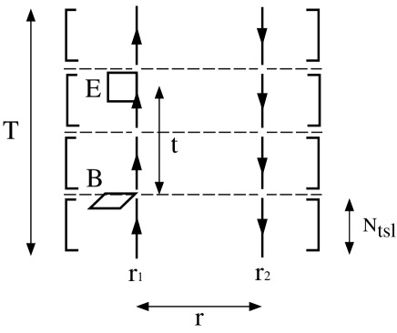
Figure 1: How to complete $\langle\!\langle g^{2}B_{y}(\vec{r}_{1},t_{1})E_{z}(\vec{r}_{1},t_{2})\rangle\!\rangle$ on the PLCF for $V_{1}^{\prime}(r)$. Arrows at $\vec{r}_{1}$ and $\vec{r}_{2}$ represent the Polyakov lines for the static quark and antiquark. $[\cdots]$ implies the sublattice average. Other field strength correlators are obtained in a similar way.

In order to benefit from the multi-level algorithm, we need to optimize $N_{\textrm{tsl}}$ and $N_{\textrm{iupd}}$. They depend on the coupling $\beta$ and on the distances to be investigated, which can be determined by looking at the behavior of the correlation function as a function of $N_{\textrm{iupd}}$ for several $N_{\textrm{tsl}}$. As an empirical observation we note that $aN_{\textrm{tsl}}=0.3-0.4$ fm is optimal in order to suppress the statistical fluctuation of the correlation functions.

In principle, one can apply the above computation to any direction of the quark-antiquark axis, $\vec{r}=(r_{x},r_{y},r_{z})$ with $r=\sqrt{r_{x}^{2}+r_{y}^{2}+r_{z}^{2}}$. However, one needs to take into account the fact that even with the simplest parametrization, $\vec{r}=(r,0,0)$, this algorithm requires a lot of memory to keep all $\mathbb{T}$ listed in Table 1 during the internal update. For a fixed distance and a fixed quark-antiquark axis using single precision, $\mathbb{T}_{PP}$ requires memory space $(L/a)^{3}\times N_{\textrm{sub}}\times 162\times 4$ bytes ($\equiv 1$ work space unit wsu). Therefore, to compute all spin-dependent potentials in the same setting, one needs additionally $5N_{\textrm{tsl}}$ wsu for the single- and $4(2N_{\textrm{tsl}}-1)$ wsu for the double-field-strength-inserted sublattice correlators. For instance, on the $20^{3}40$ lattice with $N_{\textrm{tsl}}=4$ ($N_{\textrm{sub}}=8$), about $49~{}{\it wsu}~{}=2$ GB memory is needed as $1~{}{\it wsu}=42$ MB.

The way of obtaining the HM factors $Z_{E_{z}}$, $Z_{B_{y}}$ and $Z_{B_{z}}$ using the multi-level algorithm is the same as above; we evaluate the sublattice average of $\mathbb{T}_{P\bar{B}_{x}}$, $\mathbb{T}_{P\bar{B}_{y}}$ and $\mathbb{T}_{P\bar{E}_{z}}$ and complete the correlators in Eq. (2.21). The additional memory requirement is $3N_{\textrm{tsl}}$ wsu in the above setting.

3 Numerical results

In this section, we present our numerical results. Simulation parameters are summarized in Table 2. We investigated the bare gauge couplings $\beta=6.0$ ($a\approx 0.093$ fm) on several lattice volumes and $\beta=6.3$ ($a\approx 0.059$ fm) on a $24^{4}$ lattice. The physical lattice spacing $a$ was fixed in terms of the Sommer scale by setting $r_{0}=0.5$ fm [37]. One Monte Carlo update consisted of a combination of 1 HB and 5 OR steps. The number of internal updates $N_{\textrm{iupd}}$ for each $\beta$ value was optimized empirically to obtain signals up to intermediate distances. We note that $N_{\textrm{tsl}}$ and $N_{\textrm{iupd}}$ could further be tuned so that even larger distances become accessible. The statistical errors were estimated by applying the single elimination jackknife analysis. The various fit parameters were determined by minimizing $\chi^{2}$ defined with the full covariance matrix, and their errors were estimated from the distribution of the jackknife samples. For a consistency check we also evaluated the errors of the fit parameters from the minimum value of the $\chi^{2}$ through $\Delta\chi_{\rm min}^{2}=1$. In general, the errors from the jackknife analysis were the same or slightly larger compared to those estimated from $\Delta\chi_{\rm min}^{2}=1$.

Table 2: Simulation parameters used in this study. The fourth column denotes the available quark-antiquark distances for the static potential $V_{0}$ (before tree-level improvement), while $[\cdots]$ applies to the spin-dependent potentials $V_{1}^{\prime}$, $V_{2}^{\prime}$, $V_{3}$ and $V_{4}$.

$\beta=6/g^{2}$	$a$ [fm]	$(L/a)^{3}(T/a)$	$r/a$	$N_{\rm tsl}$	$N_{\rm iupd}$	$N_{\rm conf}$
6.0	0.093	$16^{4}\phantom{1}\phantom{1}$	$2-7~{}[2-6]$	4	10000	90
6.0	0.093	$20^{4}\phantom{1}\phantom{1}$	$2-9~{}[2-6]$	4	7000	82
6.0	0.093	$20^{3}40$	$2-9~{}[2-7]$	4	7000	33
6.3	0.059	$24^{4}\phantom{1}\phantom{1}$	$2-8~{}[2-6]$	6	6000	39

3.1 Static potential and its derivatives

Figure 2: Static potential $V_{0}(r_{I})$ at $\beta=6.0$ on the $20^{3}40$ lattice and at $\beta=6.3$ on the $24^{4}$ lattice. The constant term is subtracted. The dotted line is the fit curve Eq. (3.7), applied to the data at $\beta=6.0$.

Figure 3: The force $V_{0}^{\prime}(\bar{r})$. The dotted line is the fit curve Eq. (3.8), applied to the data at $\beta=6.0$.

We first present the basic quantities extracted from the PLCF, i.e. the static potential and its derivatives with respect to the distance, in Figs. 3-4, which are defined by

$$V_{0}(r_{I}) = -\frac{1}{T}\ln\langle P(\vec{0})P^{*}(\vec{r})\rangle+O(e^{-(\Delta E_{10})T})\;,$$ (3.1)

$$V_{0}^{\prime}(\bar{r}) = \frac{1}{a}\left\{V_{0}(r)-V_{0}(r-a)\right\}\;,$$ (3.2)

$$\frac{1}{2}\tilde{r}^{3}V_{0}^{\prime\prime}(\tilde{r}) = \frac{1}{2}\tilde{r}^{3}\frac{1}{a^{2}}\left\{V_{0}(r+a)+V_{0}(r-a)-2V_{0}(r)\right\}\equiv-c(\tilde{r})\;.$$ (3.3)

We have applied tree-level improvement to the quark-antiquark distances in order to avoid an enhancement of lattice discretization effects especially at small distances [38, 37, 32], so that the distances, $r_{I}$, $\bar{r}$ and $\tilde{r}$ are defined through the relations

$$r_{I}^{-1}=4\pi G(r)\;,$$ (3.4)

$$\bar{r}^{-2}=\frac{4\pi}{a}\left\{G(r-a)-G(r)\right\}\;,$$ (3.5)

$$\tilde{r}^{-3}=\frac{2\pi}{a^{2}}\left\{G(r+a)+G(r-a)-2G(r)\right\}\;,$$ (3.6)

where $G(r)\equiv G(r,0,0)$ is the Green function of the lattice Laplacian in three dimensions. For convenience we summarize these distances in Table 6 in the Appendix.

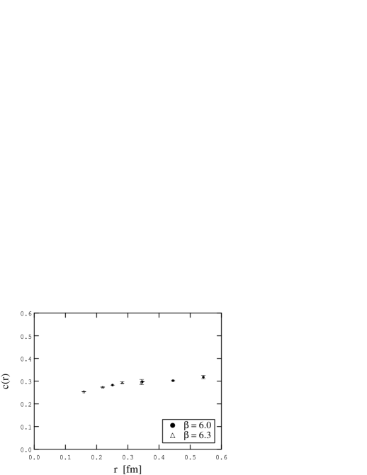
Figure 4: $c(\tilde{r})=-\tilde{r}^{3}V_{0}^{\prime\prime}(\tilde{r})/2$.

We then fit the potential and the force (first derivative of the potential) to the functions

$$V_{\mathrm{fit}}(r)=\sigma r-\frac{c}{r}+\mu\;,$$ (3.7)

$$V^{\prime}_{\mathrm{fit}}(r)=\sigma+\frac{c}{r^{2}}\;,$$ (3.8)

and estimate the string tension $\sigma$, the Coulombic coefficient $c$, and a constant $\mu$. The fit results at $\beta=6.0$ are summarized in Table 3. We find that the string tensions determined from either the potential or the force are consistent with each other. There is a small difference in $c$. However, this may be acceptable, since we see that $c(\tilde{r})$, which is extracted from the second derivative of the static potential, is not strictly constant as a function of $r$ as shown in Fig. 4. Thus $c$ can be affected by the additional fit terms. Also, given that the estimates for $c$ have not stabilized in the considered range of distances, it is not too surprising that a fit ansatz based on Eqs. (3.7) and (3.8) produces a large value of $\chi^{2}$. Nevertheless, it is interesting to find that the fit curves characterize the global feature of the potential and the force. In these fits, we found no strong dependence on the fit range. We also examined the force obtained by the central derivative $V_{0}^{\prime}(\bar{r}_{c})=\{V_{0}(r+a)-V_{0}(r-a)\}/(2a)$, where $\bar{r}_{c}$ is defined via $\bar{r}_{c}^{-2}=4\pi\{G(r-a)-G(r+a)\}/(2a)$, and found the same curve as in Fig. 3. Later, we shall compare the values of $\sigma$ and $c$ with those extracted from the spin-dependent potentials.

Table 3: Fit results of the static potential and the force at $\beta=6.0$ on the $20^{3}40$ lattice with the fit functions in Eqs. (3.7) and (3.8). The corresponding fit curves are plotted in Figs. 3 and 3.

	Fit range ($r/a$)	$\sigma a^{2}$	$c$	$\mu a$	$\chi_{\rm min}^{2}/N_{\rm df}$
$V_{0}(r)$	$1.855-8.971$	0.0466(2)	0.281(5)	0.7169(5)	3.8
$V_{0}^{\prime}(r)$	$3.312-8.438$	0.0468(2)	0.297(1)	—	5.6

At large enough distances, one may expect the value $c=\pi/12\approx 0.262$ from the bosonic string theory in four dimensions [39, 40]. However, as is clear from the plot of $c(\tilde{r})$ in Fig. 4, we find $c(\tilde{r})\approx 0.3$ at $r\gtrsim 0.3$ fm, which differs from this expectation by about 13 %. To accommodate a value of $\pi/12$ for the coefficient of the $1/r$ term, one would need higher order corrections at these distances. Note that the results for $c(\tilde{r})$ obtained here are consistent with Refs. [32, 41].

3.2 HM renormalization factors

In Fig. 5, we show the HM renormalization factors defined in Eq. (2.21), together with the tadpole renormalization factor (see Table 7 in the Appendix for the numerical values). $Z_{B_{i}}$ are almost constant as a function of $r$, while $Z_{E_{i}}$ exhibit some dependences on $r$ and on the relative orientation of the operator to the quark-antiquark axis at smaller distances. The HM factors are generally smaller than the tadpole factor by less than 1 % for $Z_{B_{i}}$ and at most 6 % for $Z_{E_{i}}$. Since the statistical fluctuations of these factors are much smaller than that of the field strength correlators, we ignore their errors when we multiply them to the field strength correlators, but take into account their $r$-dependences. Note that the observed tendencies are in agreement with Ref. [30], where the Wilson loop was used.

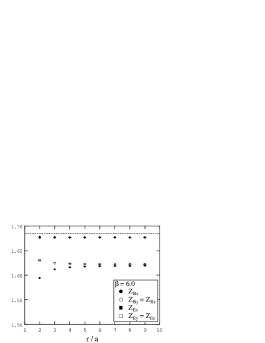
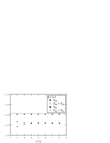
Figure 5: The HM factors at $\beta=6.0$ (left) and $\beta=6.3$ (right) as a function of $r$. The dashed lines correspond to the tadpole estimate from the inverse of the expectation value of the plaquette: $Z_{\rm tad}=1.684$ ($\langle U_{\Box}\rangle=0.59373(4)$) at $\beta=6.0$ and $Z_{\rm tad}=1.607$ ($\langle U_{\Box}\rangle=0.62241(2)$) at $\beta=6.3$.

3.3 Field strength correlators

In Figs. 6 and 7, we show the various field strength correlators as a function of $t$ at $\beta=6.0$ on the $20^{4}$ and $20^{3}40$ lattices, respectively, where $r/a=5$ is selected as an example. At smaller distances, the quality of the data is even better. Owing to the multi-level algorithm, the statistical accuracy of the data is unprecedented, which allows us see the typical behavior of correlators.

We also include the fit curves in these figures, which are supplied by the spectral representation of the field strength correlators on the PLCF in subsection 2.1. We find that Eqs. (2.8)-(2.10) provide an excellent description of the behavior of the lattice data. Our fit procedure was as follows. We first folded the data of $C(t)=\langle\!\langle g^{2}B_{y}(\vec{0},0)E_{z}(\vec{0},t)\rangle\!\rangle$ and $\langle\!\langle g^{2}B_{y}(\vec{0},0)E_{z}(\vec{r},t)\rangle\!\rangle$ as $\{C(t)-C(T-t)\}/2\to C(t)$ with $t\in[0.5a,(T-a)/2]$, and the data of $C(t)=\langle\!\langle g^{2}B_{x}(\vec{0},0)B_{x}(\vec{r},t)\rangle\!\rangle$ and $\langle\!\langle g^{2}B_{y}(\vec{0},0)B_{y}(\vec{r},t)\rangle\!\rangle$ as $\{C(t)+C(T-t)\}/2\to C(t)$ with $t\in[0,T/2]$. Then, we fitted all available data points for each correlator in order to take into account as many excited states as possible in the spectral representations, except for $t/a=0.5$ in $\langle\!\langle g^{2}B_{y}(\vec{0},0)E_{z}(\vec{0},t)\rangle\!\rangle$, which was to avoid unwanted lattice effects due to the sharing of the same link variable in the two field strength operators. Here, since it is impossible to fix the parameters, matrix elements and the energy gaps, for all excited states, $m\geq 1$, with a finite number of data points, we truncated the expansion at a certain $m=m_{\rm max}$. The validity of this truncation was verified by monitoring the values of $\chi^{2}$ and the integration results. We generally chose $m_{\rm max}$ such that $\chi_{\rm min}^{2}/N_{\rm df}$ was of order 1, where $N_{\rm df}$ is the number of degrees of freedom. All fit details and the fit results (i.e. the values of the integral) are tabulated in Tables 8 and 9 in the Appendix.

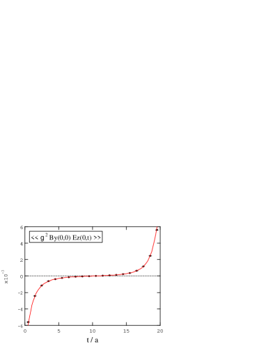
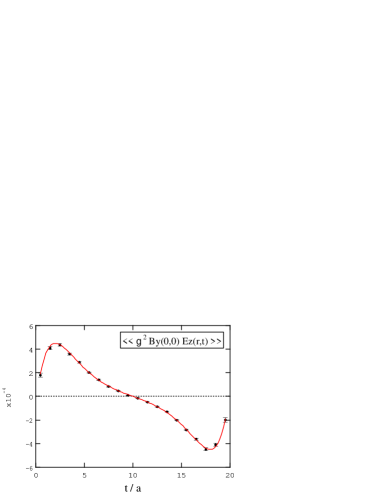
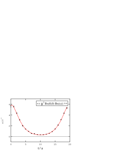
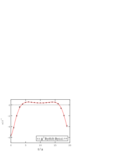
Figure 6: Field strength correlators at $\beta=6.0$ on the $20^{4}$ lattice for $r/a=5$ as a function of $t/a$. The solid lines are the fit curves corresponding to Eqs. (2.8)-(2.10).

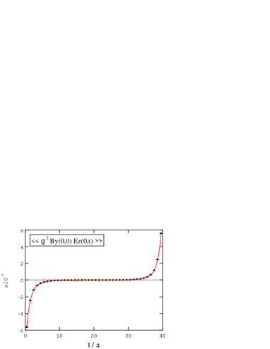
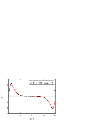
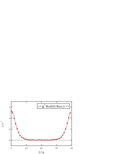
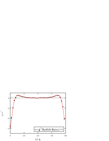
Figure 7: The same as Fig. 6 but on the $20^{3}40$ lattice.

An important observation is that the integrals obtained for $T=20a$ and $T=40a$ are the same within errors, despite the fact that the behavior of the correlators around $t=T/2$ in Figs. 6 and 7 is obviously different. While the correlator computed for $T=20a$ is clearly distorted due to periodicity, this is not the case for $T=40a$ (note that the vertical axis is the same in both figures). This indicates that the hyperbolic sine or cosine function in the spectral representation provides a good description of the finite-$T$ effect. In other words, it is possible to extract the asymptotic value of the integral from the lattice with a relatively small value of $T$ within this approach. At the same time, this confirms that the error term of $O(e^{-(\Delta E_{10})T})$ is negligible in this setting. We also examined a smaller lattice volume, $16^{4}$, at $\beta=6.0$ and obtained the same result at $r/a\leq 6$. In this sense the spatial finite volume effect at $r/a\leq 6$ on the $20^{4}$ and $20^{3}40$ lattices is also negligible.

The fit result at $\beta=6.3$ on the $24^{4}$ lattice is listed in Table 10 in the Appendix. The finite volume effect at this $\beta$ value is expected to be small, though we did not investigate this explicitly, since the physical size of the lattice volume is almost the same as for $16^{4}$ at $\beta=6.0$.

Finally, we point out several caveats. i) Although the fit works beautifully, one may not be able to assign a quantitative meaning to the resulting matrix elements and the energy gaps. This is because we truncated the spectral representation when performing the fit, and as a result, the lattice data, which in principle contains the contribution from all modes, are forced to be described by only a few modes. In this case, it is reasonable to regard only the value for the integral to be of quantitative significance. ii) As the energy gaps of the various field strength correlators in Eqs. (2.8)-(2.10) are the same, one may expect that the fit of each correlator provides the same energy gap, or one may attempt a simultaneous fit of all correlators with such a constraint. However, as the effective truncation level is not always common to all correlators, even at a fixed distance, which is also related to the fact that the matrix elements are not positive definite, this was not always the case. iii) The sensitivity of the fit result, namely the integration value, is mostly governed by the lowest energy gap selected by the fit, which gives the dominant contribution at $\tau\to\infty$. This is why we examined two lattice volumes with the same spatial size but different temporal extent and confirmed that such a systematic effect is negligible. This fact supports our claim that the spectral representation of the field strength correlator is useful even though a truncation must necessarily be performed.

3.4 Spin-dependent potentials

The spin-dependent potentials, $V_{1}^{\prime}(r)$, $V_{2}^{\prime}(r)$, $V_{3}(r)$ and $V_{4}(r)$ at $\beta=6.0$ on the $20^{3}40$ lattice and at $\beta=6.3$ on the $24^{4}$ lattice are presented in Figs. 9, 9, 13 and 13, respectively, expressed in physical units. These are the main results of this paper. Though we expect a scaling behavior for $V_{\rm SD}(r)$ in Eq. (1.1), both data at $\beta=6.0$ and $\beta=6.3$ for each potential seem to fall into one curve, which in turn may indicate that the matching coefficients should depend weakly on $\beta$. The qualitative behavior of these potentials is not obscured by numerical errors. However, there is still room for improvement for the data with $r>0.3$ fm at $\beta=6.3$. The raw data in the lattice unit are summarized in Tables 11-13 in the Appendix. The rest of this subsection is devoted to the interpretation of our data. In particular, we shall discuss the functional form of the dependence of the potentials on the distance $r$.

We start by briefly summarizing the theoretical expectation for the spin-dependent potentials. As mentioned in the introduction, Gromes derived a relation between the static potential and the spin-orbit potentials, $V^{\prime}_{0}(r)=V^{\prime}_{2}(r)-V^{\prime}_{1}(r)$, using the Lorentz (Poincaré) invariance of the field strength correlators [18, 19]. He also derived several inequalities for the spin-spin potentials based on reflection positivity, such as $V_{3}(r)\geq V_{4}(r)$ and $2V_{3}(r)+V_{4}(r)\geq 0$ [42]. These relations are nonperturbative, and can thus be checked directly on the lattice. Moreover, these relation do not depend on the matching scale.

Another source of information comes from the systematic non-relativistic reduction of the Bethe-Salpeter (BS) equations within the instantaneous approximation [1]. Starting from the interaction kernel, which is assumed to be a function of the norm squared of the relative momentum between a quark and an antiquark with various Lorentz structures, one arrives at a Breit-Fermi type effective Hamiltonian up to $O(1/m^{2})$ [43, 44]. By comparing this effective Hamiltonian with Eq. (1.1) (where $C_{F}^{(i)}=1$ is assumed), one obtains the relation between the Lorentz structure of the kernel and the spin-dependent potentials as summarized in Table 4. This indicates that the Lorentz structure of the confining static potential can also be inferred from the structure of the spin-dependent potentials. For the special case of the one-gluon-exchange interaction, the kernel only consists of the Lorentz vector, and the spin-dependent potentials are explicitly given by

$$V_{1}^{\prime}(r)=0\;,\quad V^{\prime}_{2}(r)=\frac{c}{r^{2}}\;,\quad V_{3}(r)=\frac{3c}{r^{3}}\;,\quad V_{4}(r)=8\pi c\delta^{(3)}(r)\;,\quad\quad$$ (3.9)

where $c=C_{F}\alpha_{s}$.

Table 4: The relation between the Lorentz structure of the effective kernel in the Bethe-Salpeter equation and the spin-dependent potentials [1]. $S(r)$, $V(r)$ and $P(r)$ are some scalar functions. If the interaction kernel has several components, the expected forms of the potentials are given by the sum of the corresponding terms.

Kernel	$V_{0}(r)$	$V_{1}(r)$	$V_{2}(r)$	$V_{3}(r)$	$V_{4}(r)$
Scalar	$S(r)$	$-S(r)$	$0$	0	0
Vector	$V(r)$	0	$V(r)$	$-V^{\prime\prime}(r)+V^{\prime}(r)/r$	$2\Delta V(r)$
Pseudo-scalar	0	0	0	$P^{\prime\prime}(r)-P^{\prime}(r)/r$	$\Delta P(r)$

We shall now investigate the $r$-dependence of our lattice data in more detail. We emphasize that, apart from the Gromes relation, no exact predictions exist for the behavior of the potentials beyond the short-distance regime. We have thus investigated the $r$-dependence of the potential by fitting the data to a particular model function, mostly guided by the short-distance predictions of Eq. (3.9). In cases where the latter clearly failed to describe the data, we have also resorted to effective parametrizations. The quality of a particular fit ansatz was judged by monitoring the value of $\chi^{2}_{\rm min}/N_{\rm df}$ as computed using the full covariance matrix. Clearly, the underlying mechanism responsible for the observed behavior cannot be established rigorously in this manner. However, the main aim of this analysis is to provide nonperturbative input and guidance for future conceptual studies in this area.

In the following we concentrate mostly on the dataset at $\beta=6.0$, since it extends to larger distances compared with the data collected at $\beta=6.3$. On the other hand, at smaller distances the results may be affected more by lattice artefacts. Indeed, around $r\approx 0.2$ fm we occasionally observe small discrepancies for some potentials. Therefore, in the fits to the $\beta=6.0$ dataset described below, we have mostly omitted the data point corresponding to the smallest separation $r/a=2$.

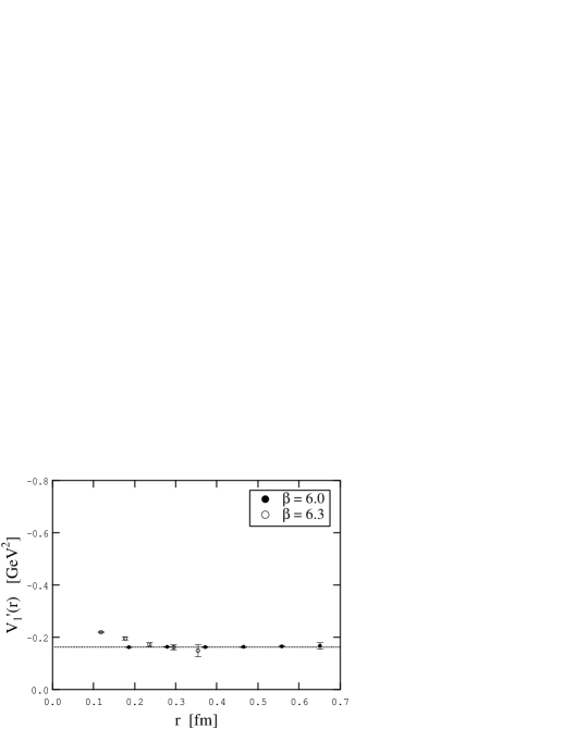
Figure 8: Spin-orbit potential $V_{1}^{\prime}(r)$ at $\beta=6.0$ and $\beta=6.3$. The dotted line is the fit curve Eq. (3.10), applied to the data of $\beta=6.0$.

Figure 9: Spin-orbit potential $V_{2}^{\prime}(r)$ at $\beta=6.0$ and $\beta=6.3$. The dotted line is the fit curve Eq. (3.8), applied to the data of $\beta=6.0$.

We start our discussion with the spin-orbit potentials $V_{1}^{\prime}(r)$ and $V_{2}^{\prime}(r)$. For $V_{1}^{\prime}(r)$, we find that the potential is negative and almost constant at $r\gtrsim 0.25$ fm (see Fig. 9). This behavior clearly contradicts Eq. (3.9) and suggests the existence of the Lorentz-scalar piece in the interaction kernel in terms of the BS equation. Our data at $\beta=6.3$ suggest that one cannot exclude a deviation from a constant at small distances, an observation which was also made by Bali et al. [29, 30]. For $V_{2}^{\prime}(r)$, we see a decreasing behavior with $r$ (see Fig. 9), which is not restricted to the short range, but rather seems to have a finite tail up to intermediate distances.

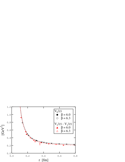
Figure 10: Comparison between the force $V_{0}^{\prime}(r)$ and the difference of the spin-orbit potentials $V_{2}^{\prime}(r)-V_{1}^{\prime}(r)$ at $\beta=6.0$ on the $20^{3}40$ lattice and $\beta=6.3$ on the $24^{4}$ lattice with the physical scale. The Gromes relation is $V_{0}^{\prime}(r)=V_{2}^{\prime}(r)-V_{1}^{\prime}(r)$. The dotted line is the fit curve for the force $V_{0}^{\prime}$, while the dashed line is for $V_{2}^{\prime}-V_{1}^{\prime}$, where Eq. (3.8) is used in both cases.

Figure 11: The relative deviation from the Gromes relation, $1-(V_{2}^{\prime}-V_{1}^{\prime})_{\rm fit}/V_{\rm 0;fit}^{\prime}$, at $\beta=6.0$. The fit functions are the same as in Fig. 11 and the dotted lines denote the $1\sigma$ error band.

Before discussing the functional form of $V_{1}^{\prime}(r)$ and $V_{2}^{\prime}(r)$ quantitatively, we may ask if these spin-orbit potentials satisfy the Gromes relation, since otherwise it is unclear whether any quantitative arguments make sense. In Fig. 11, we compare the static force, $V_{0}^{\prime}(r)$, with the difference of the spin-orbit potentials, $V_{2}^{\prime}(r)-V_{1}^{\prime}(r)$. We find quite a good agreement, indicating that the Gromes relation is apparently satisfied. We can examine this relation in more detail by fitting the difference $V_{2}^{\prime}(r)-V_{1}^{\prime}(r)$ at $\beta=6.0$ to the same functional form as the force in Eq. (3.8). Thereby we obtain $\sigma_{\rm v21}a^{2}=0.0426(9)$ and $c=0.293(9)$ with $\chi^{2}_{\rm min}/N_{\rm df}=0.26$.  The string tension extracted in this way is about 8 % smaller than that in $V_{0}^{\prime}(r)$, while the Coulombic coefficients are in agreement within errors. We also plot the quantity $1-(V_{2}^{\prime}-V_{1}^{\prime})_{\rm fit}/V_{\rm 0;fit}^{\prime}$ in Fig. 11. From this we conclude that the Gromes relation is satisfied within $(8\pm 1)$ % accuracy at $r\approx 0.5$ fm. Note that without the renormalization factor for the field strength operator, one would observe a strong deviation from the Gromes relation by a factor $\approx 2.7$ at $\beta=6.0$. In this sense, the renormalization of the operator is crucial for satisfying the Gromes relation within a few percent level, especially when the lattice spacing is finite. It is certainly interesting to investigate if the Gromes relation is exactly satisfied in the continuum limit. Although we have investigated the gauge coupling at $\beta=6.3$, we need further accuracy of the data at intermediate distances to achieve this.

For $V_{1}^{\prime}(r)$, if we only take into account the data for $r\gtrsim 0.25$ fm at $\beta=6.0$ and, assuming that they are constant, we can fit them to a function

$$V^{\prime}_{\rm 1;fit}=-\sigma_{\rm v1}\;.$$ (3.10)

Due to the Gromes relation, we may identify this constant as a part of the string tension in $V_{0}^{\prime}(r)$. We then find $\sigma_{\rm v1}a^{2}=0.0362(4)$ with $\chi^{2}_{\rm min}/N_{\rm df}=0.13$, which is $(77\pm 1)$ % of the string tension in $V_{0}^{\prime}(r)$. The corresponding fit curve is plotted in Fig. 9.

While the Gromes relation is approximately satisfied, we find that the string tension $\sigma_{\rm v1}$ is not yet sufficient to reproduce the string tension $\sigma_{\rm v21}$. In other words there is still a missing amount of the string tension. We then notice that this must be supplied by $V_{2}^{\prime}(r)$. A fit of $V_{2}^{\prime}(r)$ to Eq. (3.8) indeed leads to $\sigma_{\rm v2}a^{2}=0.0070(7)$ and $c=0.288(7)$ with $\chi^{2}_{\rm min}/N_{\rm df}=0.22$. The fit curve is plotted in Fig. 9. Now the sum of $\sigma_{\rm v1}$ and $\sigma_{\rm v2}$ reproduces $\sigma_{\rm v21}$. These findings suggest the existence of a long-ranged contribution in $V_{2}^{\prime}(r)$ whose magnitude is about one-fifth of $\sigma_{\rm v1}$, which is $(15\pm 2)$ % of the string tension in $V_{0}^{\prime}(r)$. We also attempted a fit with the expectation from perturbation theory, by simply fixing the string tension to be zero in the above fit. In this case the fit clearly fails, since $\chi^{2}_{\rm min}/N_{\rm df}=44$. From the phenomenological point of view, one might prefer a simple parametrization like $\sigma=\sigma_{\rm v1}$ and $\sigma_{\rm v2}=0$ [45], but the results obtained here slightly differ from this expectation. We wish to point out, though, that $V^{\prime}_{2}(r)$ should further be investigated at distances larger than 0.7 fm, in order to corroborate a non-vanishing value of $V^{\prime}_{2}(r)$ for $r\to\infty$. We may note that Eq. (3.8) is not the only functional form for $V_{2}^{\prime}(r)$. For instance, the function $V_{\rm 2;fit}^{\prime}(r)=c^{\prime}/r^{p}$ with $p=1.51(4)$ and $c^{\prime}a^{p-2}=0.205(9)$ also reproduces the data quite well, with $\chi^{2}_{\rm min}/N_{\rm df}=0.34$.

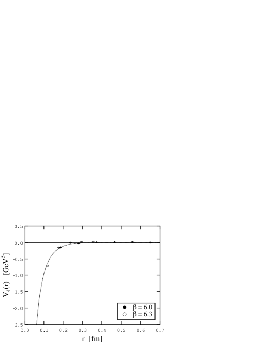
Figure 12: Spin-spin (tensor) potential $V_{3}(r)$ at $\beta=6.0$ and $\beta=6.3$. The dotted line is the fit curve Eq. (3.11), applied to the data of $\beta=6.0$.

Figure 13: Spin-spin potential $V_{4}(r)$ at $\beta=6.0$ and $\beta=6.3$. The dotted line is the fit curve Eq. (3.12), applied to the data of $\beta=6.0$.

Next, we discuss the spin-spin potentials $V_{3}(r)$ and $V_{4}(r)$. We first examine $V_{3}(r)$ (see Fig. 13) if the ansatz motivated by one-gluon-exchange in Eq. (3.9) is appropriate. The fit to this function yields the coefficient $c=0.214(2)$ with $\chi_{\rm min}^{2}/N_{\mathrm{df}}=3.7$. This value of $\chi_{\rm min}^{2}/N_{\mathrm{df}}$ is relatively large and the result for $c$ is 28 % smaller than the Coulombic coefficient in $V_{0}^{\prime}(r)$. A better fit can be achieved using an ansatz in which the power of $1/r$ is left as a free parameter, i.e.

$$V_{\rm 3;fit}(r)=\frac{3c^{\prime}}{r^{p}}\;.$$ (3.11)

This yields $c^{\prime}a^{p-3}=0.171(10)$ and $p=2.80(6)$, where $\chi_{\rm min}^{2}/N_{\mathrm{df}}=0.79$. The corresponding fit curve is plotted in Fig 13. The value of $p$ is smaller than $3$ within 3 standard deviations. If one takes this result as face value, it indicates a deviation from the one-gluon-exchange potential. A deviation might actually be expected from the existence of the long-ranged contribution in $V_{2}^{\prime}(r)$ and the relations in Table 4; if we insert a function $V(r)=-c/r+\sigma_{\rm v2}r$ into $-V^{\prime\prime}(r)+V^{\prime}(r)/r$, we obtain $3c/r^{3}+\sigma_{\rm v2}/r$ at $r\neq 0$. We have then examined if this function describes the data for given $c$ and $\sigma_{\rm v2}$, which are supplied from the $V_{2}^{\prime}(r)$ fit. However, we have found that the resulting curve is not appropriate to describe the behavior of the data at all, since it lies above the data points at small distances. This tendency is practically due to the term $1/r^{3}$, but this additional term $1/r$ also helps to lift the curve. It suggests that we need to add a negative contribution to such an ansatz.

A possible candidate would then be a pseudo-scalar contribution, which is also closely related to the behavior of $V_{4}(r)$ (see Fig. 13). In fact, if only the one-gluon-exchange interaction is considered in the vector kernel, $2\Delta V(r)=2(V^{\prime\prime}(r)+2V^{\prime}(r)/r)$ leads to a $\delta$-function as in Eq. (3.9), while if we insert the empirical behavior of $V_{2}^{\prime}(r)$, an additional term of $4\sigma_{\rm v2}/r$ is generated for $V_{4}(r)$. Thus we expect a positive behavior at non-zero distances. By contrast, the data is negative at small distances and almost zero for $r>0.2$ fm. Let us now assume the presence of a pseudo-scalar interaction, $P(r)=-g^{\prime}e^{-m_{g}r}/r$, where $m_{g}$ is the mass of the lightest pseudo-scalar particle, and $g^{\prime}$ is the corresponding effective coupling to quarks. This certainly generates a negative contribution, $\Delta P(r)=-g^{\prime}m_{g}^{2}e^{-m_{g}r}/r$, to $V_{4}(r)$. Note that the pseudo-scalar interaction $P(r)$ is often used in the one-boson-exchange model for describing the nucleon-nucleon system, where pions play a relevant role [46]. In our simulation, however, since the effects of dynamical fermions are neglected due to our use of the quenched approximation, the lowest mass in the pseudo-scalar channel cannot be identified with the pion mass but rather with the lightest glueball mass.

We have then performed a fit to

$$V_{\rm 4;fit}(r)=-g^{\prime}m_{g}^{2}\frac{e^{-m_{g}r}}{r}+4\frac{\sigma_{\rm v4}}{r}\;,$$ (3.12)

where we have assumed $m_{g}=2.47$ GeV, which is taken from the recent lattice studies of the glueball masses [47], and treated $g^{\prime}$ and $\sigma_{\rm v4}$ as free parameters. The result was $g^{\prime}=0.292(12)$ and $\sigma_{\rm v4}a^{2}=0.0015(3)$ with $\chi_{\rm min}^{2}/N_{\mathrm{df}}=5.1$, and the corresponding curve is put in Fig. 13 (if $m_{g}$ is relaxed to be a free parameter, $\chi_{\rm min}^{2}/N_{\rm df}$ is significantly reduced). We find that $\sigma_{\rm v4}$ (notice that this value is not zero) is not exactly $\sigma_{\rm v2}$, but as the relation among interaction kernels is not exact but derived within the instantaneous approximation, such a deviation may occur, especially for the nonperturbative pieces. On the other hand, the value of $g^{\prime}$ is very close to $c=0.297(1)$ determined from the force (see Table 3). If we impose $\sigma_{\rm v4}=\sigma_{\rm v2}$, we obtain here $\chi_{\rm min}^{2}/N_{\mathrm{df}}\approx 100$. However the apparent shape of the curve is not affected so much as is mostly governed by the glueball mass we set.

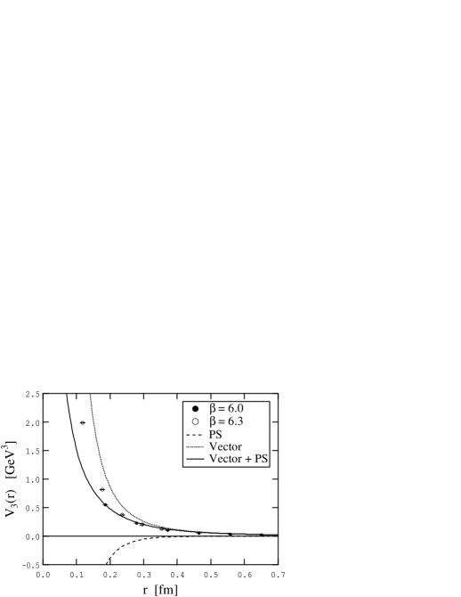
Figure 14: A possible structure of the spin-spin potential $V_{3}(r)$. The lattice data are the same as in Fig. 13. The dotted (dashed) line corresponds to the vector (pseudo-scalar) contribution, Eq. (3.13) (Eq. (3.14)) and the sum of these two contributions is indicated by the solid line.

Figure 15: $r(2V_{3}+V_{4})-6V_{2}^{\prime}$ at $\beta=6.0$.

Now we come back to $V_{3}(r)$ and examine if the sum of the (positive) vector and the (negative) pseudo-scalar contributions, with parameters estimated by the $V_{4}(r)$ fit, can describe the behavior of $V_{3}(r)$. Here, we consider the sum of two functions,

$$V_{3}^{\rm(V)}(r)=\frac{3c}{r^{3}}+\frac{\sigma_{\rm v4}}{r}\;,$$ (3.13)

$$V_{3}^{\rm(PS)}(r)=P^{\prime\prime}(r)-\frac{P^{\prime}(r)}{r}=-g^{\prime}(\frac{3}{r^{3}}+\frac{3m_{g}}{r^{2}}+\frac{m_{g}^{2}}{r})e^{-m_{g}r}\;,$$ (3.14)

where $c$ is taken from $V_{0}^{\prime}(r)$. It is interesting to see Fig. 15 that the curve $V_{3}^{\rm(V)}(r)+V_{3}^{\rm(PS)}(r)$, which is plotted with the solid line, can go through the data at $\beta=6.0$.

Table 5: Fit results of the spin-dependent potentials at $\beta=6.0$ on the $20^{3}40$ lattice. (*) if we relax $m_{g}$ to be a free parameter, $\chi_{\rm min}^{2}/N_{\mathrm{df}}$ is significantly reduced.

Potential	Fit range ($r/a$)	Fit function and parameters	$\chi_{\rm min}^{2}/N_{\mathrm{df}}$
$V_{1}^{\prime}(r)$		$V_{\mathrm{fit}}^{\prime}=-\sigma$
	$3-7$	$\sigma a^{2}=0.0362(4)$	0.13
$V_{2}^{\prime}(r)$		$V_{\mathrm{fit}}^{\prime}(r)=\sigma+c/r^{2}$
	$3-6$	$\sigma a^{2}=0.0070(7)$, $c=0.288(7)$	0.22
		$V_{\mathrm{fit}}^{\prime}(r)=c^{\prime}/r^{p}$
	$3-6$	$c^{\prime}a^{p-2}=0.205(9)$, $p=1.51(4)$	0.34
$V_{2}^{\prime}(r)-V_{1}^{\prime}(r)$		$V_{\mathrm{fit}}^{\prime}(r)=\sigma+c/r^{2}$
	$3-7$	$\sigma a^{2}=0.0426(9)$, $c=0.293(9)$	0.26
$V_{3}(r)$		$V_{\mathrm{fit}}(r)=3c/r^{3}$
	$3-7$	$c=0.214(2)$	3.71
		$V_{\mathrm{fit}}(r)=3c^{\prime}/r^{p}$
	$3-7$	$c^{\prime}a^{p-3}=0.171(10)$, $p=2.80(6)$	0.79
$V_{4}(r)$		$V_{\mathrm{fit}}(r)=-g^{\prime}m_{g}^{2}e^{-m_{g}r}/r+4\sigma/r$
	$2-7$	$g^{\prime}=0.292(12)$, $\sigma a^{2}=0.0015(3)$,
		$m_{g}a=1.16$ (fixed)	5.1∗

In most of previous works, it was concluded that $V_{4}(r)$ is consistent with a $\delta$-function, which may only be true at very small distances. However, as we demonstrated, the behavior of $V_{3}(r)$ and $V_{4}(r)$ at distances $r\gtrsim 0.2$ fm can be consistently explained by assuming the existence of the pseudo-scalar contribution as well as the vector contribution. Note furthermore that the combination of the potentials $r(2V_{3}+V_{4})-6V_{2}^{\prime}$ should be zero at non-zero distances, if the interaction kernel contains only the pure vector component without a linear term and no pseudo-scalar contribution (see Table 4) [23]. However, as shown in Fig. 15, we find that this combination is non-vanishing within our accuracy, so that some of these assumptions are probably not applicable. Of course, our discussion on the pseudo-scalar contribution is as yet speculation, which needs to be checked in future works. A possible way of doing this is to investigate $V_{4}(r)$ in the presence of dynamical quarks (pions) in full QCD simulations, and to examine whether one can indeed observe a behavior like $\propto-e^{-m_{\pi}r}/r$ for sufficiently small quark masses. Some of previous works in Refs. [27, 28] have been carried out in full QCD, but the data quality is not sufficient to draw any conclusion. In any case, we expect to raise further discussions on the structure of the spin-spin potentials.

To close the discussion on the functional form, we note that the Gromes inequalities $V_{3}(r)\geq V_{4}(r)$ and $2V_{3}(r)+V_{4}(r)\geq 0$ are certainly satisfied. For instance, the latter inequality is immediately checked through $2V_{3}(r)+V_{4}(r)=6\int_{0}^{\infty}dt\langle\!\langle g^{2}B_{x}(\vec{0},0)B_{x}(\vec{r},t)\rangle\!\rangle$, which is positive at all available $r$ as can be seen from Tables 8-10 in the Appendix. We summarize all fit results of the functional form in Table 5.

4 Summary

We have investigated the spin-dependent corrections to the static potential at $O(1/m^{2})$ in SU(3) lattice gauge theory. These corrections, usually called the spin-dependent potentials, are represented as the integral of the field strength correlators on the quark-antiquark source with respect to the relative temporal distance between two field strength operators. We have used the Polyakov loop correlation function as the quark-antiquark source, and by employing the multi-level algorithm, we have obtained remarkably clean data for the expectation values of the field strength correlators and, in turn, for the spin-dependent potentials up to intermediate distances of around $r\simeq 0.6$ fm. The spectral representation of the field strength correlator in a finite periodic volume has been exploited in order to extract the potential with less systematic error.

The observation we have made for the spin-dependent potentials in Eq. (1.1) is as follows. The spin-orbit potential $V_{1}^{\prime}(r)$ is clearly long-ranged, is negative at all distances and constant at $r\gtrsim 0.25$ fm. The other spin-orbit potential $V_{2}^{\prime}(r)$ is positive at all distances and shows a behavior decreasing with $r$. However, it has a finite tail up to intermediate distances, which cannot be explained at least by the one-gluon-exchange interaction. The Gromes relation $V_{0}^{\prime}(r)=V_{2}^{\prime}(r)-V_{1}^{\prime}(r)$ is satisfied within ($8\pm 1$) % accuracy at intermediate distances in the present simulation. Within this relation, the constant value in $V_{1}^{\prime}(r)$ reproduces $(77\pm 1)$ % of the string tension in $V_{0}^{\prime}(r)$ and $(15\pm 2)$ % of the string tension are found to be supplied by $V_{2}^{\prime}(r)$. The spin-spin (tensor) potential $V_{3}(r)$ is positive at all distances and is decreasing as a function of $r$. The behavior is slightly more moderate than the expectation of the one-gluon-exchange picture $\propto 1/r^{3}$. The other spin-spin potential $V_{4}(r)$ exhibits a negative short-ranged behavior. This short-ranged behavior, as well as the behavior of $V_{3}(r)$, could be explained if the exchange of the pseudo-scalar glueball is assumed in addition to the one-gluon-exchange type interaction.

In this paper we have not carried out a detailed comparison of the lattice result of the spin-dependent potentials with perturbation theory, e.g. along the lines of Necco and Sommer for the static potential [37, 48]. In this sense, although we have observed a certain deviation from the expectation of leading order perturbation theory at intermediate distances, it is not yet clear that from which distance a perturbative description becomes inadequate. Clearly, it requires further systematic studies, where the renormalization of the field strength operator and also the matching coefficients are worth to be reconsidered. However, we expect that the numerical procedures we have demonstrated in this paper is quite useful for such a work. Then, it is interesting to use the result as inputs of phenomenological models [49, 50, 51] or to compare with the various QCD vacuum models [52, 53, 54]. It may be interesting to note that the existence of a long-ranged contribution in $V_{2}^{\prime}(r)$ is suggested in Ref. [54], independently of the present work.

Finally we note that our numerical procedures are also applicable to the evaluation of other relativistic corrections like the velocity-dependent potentials [55, 56, 11] and the potential at $O(1/m)$ [14, 15, 11, 57, 58, 59, 60, 61], which are also represented as the field strength correlators on the quark-antiquark source with different combination of the field strength operators from the spin-dependent potentials. The first lattice result on the potential at $O(1/m)$ was published in Ref. [34].

Appendix A Collection of numerical values

A.1 Tree-level improvement of the quark-antiquark distances

Table 6: The quark-antiquark distances for the static potential $V_{0}(r_{I})$, the force $V_{0}^{\prime}(\bar{r})$ (or $V_{0}^{\prime}(\bar{r}_{c})$) and the second derivative $V^{\prime\prime}_{0}(\tilde{r})$ with the tree-level improvement [38, 37, 32].

$r/a$	$r_{I}/a$	$\bar{r}/a$	$\bar{r}_{c}/a$	$\tilde{r}/a$
1	0.925
2	1.855	1.358	1.649	1.788
3	2.889	2.277	2.654	2.700
4	3.922	3.312	3.729	3.729
5	4.942	4.359	4.794	4.786
6	5.954	5.393	5.837	5.833
7	6.962	6.414	6.865	6.864
8	7.967	7.428	7.885	7.886
9	8.971	8.438	8.899	8.901

A.2 HM factors

Table 7: The HM renormalization factors at $\beta=6.0$ on the $20^{4}$ lattice (upper) and $\beta=6.3$ on the $24^{4}$ lattice (lower), where the quark-antiquark system is set along the $x$ axis. Thus, one should observe $Z_{E_{y}}=Z_{E_{z}}$, $Z_{B_{y}}=Z_{B_{z}}$.

$r/a$	$Z_{E_{x}}$	$Z_{E_{y}}$	$Z_{E_{z}}$	$Z_{B_{x}}$	$Z_{B_{y}}$	$Z_{B_{z}}$
2	1.59446(4)	1.63031(6)	1.63038(5)	1.67833(16)	1.67614(12)	1.67600(15)
3	1.61170(4)	1.62498(6)	1.62503(5)	1.67764(16)	1.67661(12)	1.67651(15)
4	1.61620(4)	1.62338(6)	1.62339(6)	1.67735(16)	1.67676 (12)	1.67669(14)
5	1.61777(6)	1.62282(6)	1.62282(7)	1.67726(16)	1.67687(13)	1.67678(15)
6	1.61846(6)	1.62250(7)	1.62262(6)	1.67721(16)	1.67695(13)	1.67683(16)
7	1.61877(10)	1.62246(8)	1.62233(8)	1.67726(16)	1.67684(13)	1.67680(15)
8	1.61879(15)	1.62225(17)	1.62232(16)	1.67708(18)	1.67682(19)	1.67674(19)
2	1.54232(3)	1.56529(3)	1.56526(3)	1.60307(7)	1.60179(9)	1.60185(7)
3	1.55417(5)	1.56151(4)	1.56154(4)	1.60271(7)	1.60217(10)	1.60226(7)
4	1.55717(6)	1.56048(4)	1.56049(6)	1.60266(7)	1.60225(10)	1.60235(7)
5	1.55810(9)	1.56013(6)	1.56004(7)	1.60260(9)	1.60231(11)	1.60231(10)
6	1.55853(10)	1.55974(11)	1.55986(13)	1.60247(11)	1.60229(12)	1.60253(11)
7	1.55829(18)	1.55921(23)	1.55980(14)	1.60238(18)	1.60216(17)	1.60223(16)
8	1.55855(40)	1.55974(37)	1.55975(32)	1.60260(29)	1.60249(28)	1.60217(23)
9	1.55961(43)	1.55954(64)	1.56021(48)	1.60324(36)	1.60324(39)	1.60331(44)

A.3 Fit results of the field strength correlators

Table 8: Fit results of the field strength correlators with Eqs. (2.8)-(2.10) at $\beta=6.0$ on the $20^{4}$ lattice. $m_{\rm max}$ is the maximum truncation level of the spectral representation.

$C(t)$	$r/a$	Fit range $(t/a)$	$m_{\rm max}$	$a^{2}\int_{0}^{\infty}dt\;tC(t)$	$\chi_{\rm min}^{2}/N_{\rm df}$
$\langle\!\langle g^{2}B_{y}(0,0)E_{z}(0,t)\rangle\!\rangle$	2	$2-10$	2	$-$0.01801(4)	0.43
	3	$2-10$	2	$-$0.01808(6)	0.99
	4	$2-10$	2	$-$0.01805(10)	0.30
	5	$2-10$	2	$-$0.01800(19)	0.45
	6	$2-10$	2	$-$0.01795(32)	1.91
$\langle\!\langle g^{2}B_{y}(0,0)E_{z}(r,t)\rangle\!\rangle$	2	$1-10$	3	0.03618(3)	2.01
	3	$1-10$	3	0.01948(4)	2.71
	4	$1-10$	3	0.01265(10)	0.81
	5	$1-10$	2	0.00917(14)	2.01
	6	$1-10$	2	0.00795(42)	0.88
$C(t)$	$r/a$	Fit range $(t/a)$	$m_{\rm max}$	$a^{3}\int_{0}^{\infty}dt\;C(t)$	$\chi_{\rm min}^{2}/N_{\rm df}$
$\langle\!\langle g^{2}B_{x}(0,0)B_{x}(r,t)\rangle\!\rangle$	2	$1-10$	3	0.01648(3)	2.21
	3	$1-10$	3	0.00743(3)	0.97
	4	$1-10$	3	0.00381(3)	0.85
	5	$1-10$	2	0.00217(3)	2.01
	6	$1-10$	2	0.00128(5)	1.81
$\langle\!\langle g^{2}B_{y}(0,0)B_{y}(r,t)\rangle\!\rangle$	2	$1-10$	3	$-$0.01226(3)	0.77
	3	$1-10$	3	$-$0.00443(3)	0.40
	4	$1-10$	3	$-$0.00155(3)	0.37
	5	$1-10$	3	$-$0.00067(3)	0.46
	6	$1-10$	3	$-$0.00033(4)	0.48

Table 9: Fit results of the field strength correlators at $\beta=6.0$ on the $20^{3}40$ lattice.

$C(t)$	$r/a$	Fit range $(t/a)$	$m_{\rm max}$	$a^{2}\int_{0}^{\infty}dt\;tC(t)$	$\chi_{\rm min}^{2}/N_{\rm df}$
$\langle\!\langle g^{2}B_{y}(0,0)E_{z}(0,t)\rangle\!\rangle$	2	$2-20$	2	$-$0.01798(13)	2.7
	3	$2-20$	2	$-$0.01809(20)	2.5
	4	$2-20$	2	$-$0.01800(27)	2.9
	5	$2-20$	2	$-$0.01809(25)	1.4
	6	$2-20$	2	$-$0.01831(40)	1.8
	7	$2-20$	2	$-$0.01853(137)	2.6
$\langle\!\langle g^{2}B_{y}(0,0)E_{z}(r,t)\rangle\!\rangle$	2	$1-20$	3	0.03618(5)	1.4
	3	$1-20$	3	0.01950(12)	5.0
	4	$1-20$	2	0.01253(18)	1.9
	5	$1-20$	2	0.00920(31)	2.4
	6	$1-20$	2	0.00703(80)	5.7
	7	$1-20$	2	0.00457(68)	2.6
$C(t)$	$r/a$	Fit range $(t/a)$	$m_{\rm max}$	$a^{3}\int_{0}^{\infty}dt\;C(t)$	$\chi_{\rm min}^{2}/N_{\rm df}$
$\langle\!\langle g^{2}B_{x}(0,0)B_{x}(r,t)\rangle\!\rangle$	2	$1-20$	3	0.01642(7)	1.5
	3	$1-20$	3	0.00742(5)	2.2
	4	$1-20$	3	0.00372(7)	1.5
	5	$1-20$	3	0.00206(6)	1.5
	6	$1-20$	2	0.00133(16)	5.5
	7	$1-20$	2	0.00071(18)	4.5
$\langle\!\langle g^{2}B_{y}(0,0)B_{y}(r,t)\rangle\!\rangle$	2	$1-20$	3	$-$0.01226(6)	3.1
	3	$1-20$	3	$-$0.00442(7)	2.3
	4	$1-20$	3	$-$0.00166(7)	2.8
	5	$1-20$	3	$-$0.00069(6)	2.6
	6	$1-20$	3	$-$0.00029(9)	1.8
	7	$1-20$	3	$-$0.00030(39)	1.9

Table 10: Fit results of the field strength correlators at $\beta=6.3$ on the $24^{4}$ lattice. (^∗)one of the excitation energies in the expansion was fixed so as to make the fit stable.

$C(t)$	$r/a$	Fit range $(t/a)$	$m_{\rm max}$	$a^{2}\int_{0}^{\infty}dt\;tC(t)$	$\chi_{\rm min}^{2}/N_{\rm df}$
$\langle\!\langle g^{2}B_{y}(0,0)E_{z}(0,t)\rangle\!\rangle$	2	$2-12$	2	$-$0.00980(10)	1.11
	3	$2-12$	2	$-$0.00872(29)	1.21
	4	$2-12$	2	$-$0.00768(30)	1.41
	5	$2-12$	2	$-$0.00727(28)	4.4∗
	6	$2-12$	2	$-$0.00664(110)	0.94
$\langle\!\langle g^{2}B_{y}(0,0)E_{z}(r,t)\rangle\!\rangle$	2	$1-12$	3	0.03145(7)	0.28
	3	$1-12$	2	0.01620(16)	3.01
	4	$1-12$	2	0.01008(37)	2.01
	5	$1-12$	2	0.00632(43)	0.85
	6	$1-12$	2	0.00446(109)	2.31
$C(t)$	$r/a$	Fit range $(t/a)$	$m_{\rm max}$	$a^{3}\int_{0}^{\infty}dt\;C(t)$	$\chi_{\rm min}^{2}/N_{\rm df}$
$\langle\!\langle g^{2}B_{x}(0,0)B_{x}(r,t)\rangle\!\rangle$	2	$1-12$	3	0.01452(3)	0.49
	3	$1-12$	3	0.00653(3)	4.41
	4	$1-12$	2	0.00332(6)	1.21
	5	$1-12$	2	0.00188(8)	0.87
	6	$1-12$	1	0.00123(12)	0.49
$\langle\!\langle g^{2}B_{y}(0,0)B_{y}(r,t)\rangle\!\rangle$	2	$1-12$	3	$-$0.01203(3)	0.95
	3	$1-12$	3	$-$0.00436(3)	1.41
	4	$1-12$	3	$-$0.00168(7)	1.51
	5	$1-12$	2	$-$0.00084(18)	4.81
	6	$1-12$	1	$-$0.00046(12)	1.81

A.4 Spin-dependent potentials

Table 11: The spin-dependent potentials at $\beta=6.0$ on the $20^{4}$ lattice.

r/a	$a^{2}V_{1}^{\prime}$	$a^{2}V_{2}^{\prime}$	$a^{3}V_{3}$	$a^{3}V_{4}$
2	$-$0.03603(8)1	0.07235(6)1	0.05749(8)1	$-$0.01607(13)
3	$-$0.03616(12)	0.03896(9)1	0.02373(8)1	$-$0.00286(14)
4	$-$0.03609(20)	0.02531(19)	0.01072(8)1	0.00143(17)
5	$-$0.03600(39)	0.01836(28)	0.00568(9)1	0.00165(14)
6	$-$0.03591(65)	0.01590(84)	0.00322(13)	0.00123(20)

Table 12: The spin-dependent potentials at $\beta=6.0$ on the $20^{3}40$ lattice.

r/a	$a^{2}V_{1}^{\prime}$	$a^{2}V_{2}^{\prime}$	$a^{3}V_{3}$	$a^{3}V_{4}$
2	$-$0.03596(25)1	0.07235(11)1	0.05736(19)1	$-$0.01620(27)1
3	$-$0.03618(41)1	0.03900(25)1	0.02368(20)1	$-$0.00284(29)1
4	$-$0.03600(54)1	0.02507(36)1	0.01075(21)1	0.00081(30)1
5	$-$0.03619(50)1	0.01840(61)1	0.00549(18)1	0.00138(27)1
6	$-$0.03662(81)1	0.01405(160)	0.00323(37)1	0.00152(47)1
7	$-$0.03706(274)	0.00914(136)	0.00203(103)	0.00021(137)

Table 13: The spin-dependent potentials at $\beta=6.3$ on the $24^{4}$ lattice.

r/a	$a^{2}V_{1}^{\prime}$	$a^{2}V_{2}^{\prime}$	$a^{3}V_{3}$	$a^{3}V_{4}$
2	$-$0.01960(19)1	0.06290(15)1	0.05310(9)1	$-$0.01910(15)
3	$-$0.01744(58)1	0.03240(31)1	0.02178(9)1	$-$0.00439(14)
4	$-$0.01539(61)1	0.02017(74)1	0.01000(16)	$-$0.00009(31)
5	$-$0.01443(79)1	0.01265(87)1	0.00546(41)	0.00038(70)
6	$-$0.01329(221)	0.00893(217)	0.00339(37)	0.00057(52)

References

• [1] W. Lucha, F.F. Schรถberl and D. Gromes, Phys. Rept. 200 (1991) 127.
• [2] W. Buchmรผllerย (Ed.), Quarkonia, Current physics-sources and comments, vol.ย 9, (North-Holland, 1992).
• [3] G.S. Bali, Phys. Rept. 343 (2001) 1, hep-ph/0001312.
• [4] N. Brambilla etย al., Heavy quarkonium physics, CERN Yellow Report (2005), hep-ph/0412158.
• [5] E. Eichten and F. Feinberg, Phys. Rev. Lett. 43 (1979) 1205.
• [6] E. Eichten and F. Feinberg, Phys. Rev. D23 (1981) 2724.
• [7] M.E. Peskin, Aspects of the dynamics of heavy quark systems, 11th Int. SLAC Summer Inst. on Particle Physics, Stanford, CA, Jul 18-26, 1983, SLAC-PUB-3273.
• [8] D. Gromes, Z. Phys. C22 (1984) 265.
• [9] Y.J. Ng, J.T. Pantaleone and S.H.H. Tye, Phys. Rev. Lett. 55 (1985) 916.
• [10] J.T. Pantaleone, S.H.H. Tye and Y.J. Ng, Phys. Rev. D33 (1986) 777.
• [11] A. Pineda and A. Vairo, Phys. Rev. D63 (2001) 054007, hep-ph/0009145, Erratum-ibid D64 (2001) 039902.
• [12] W.E. Caswell and G.P. Lepage, Phys. Lett. B167 (1986) 437.
• [13] G.T. Bodwin, E. Braaten and G.P. Lepage, Phys. Rev. D51 (1995) 1125, hep-ph/9407339, Erratum-ibid D55 (1997) 5853.
• [14] N. Brambilla, A. Pineda, J. Soto and A. Vairo, Nucl. Phys. B566 (2000) 275, hep-ph/9907240.
• [15] N. Brambilla, A. Pineda, J. Soto and A. Vairo, Phys. Rev. D63 (2001) 014023, hep-ph/0002250.
• [16] N. Brambilla, A. Pineda, J. Soto and A. Vairo, Rev. Mod. Phys. 77 (2005) 1423, hep-ph/0410047.
• [17] A.V. Manohar, Phys. Rev. D56 (1997) 230, hep-ph/9701294.
• [18] D. Gromes, Z. Phys. C26 (1984) 401.
• [19] N. Brambilla, D. Gromes and A. Vairo, Phys. Rev. D64 (2001) 076010, hep-ph/0104068.
• [20] Ph. deย Forcrand and J.D. Stack, Phys. Rev. Lett. 55 (1985) 1254.
• [21] C. Michael and P.E.L. Rakow, Nucl. Phys. B256 (1985) 640.
• [22] C. Michael, Phys. Rev. Lett. 56 (1986) 1219.
• [23] A. Huntley and C. Michael, Nucl. Phys. B286 (1987) 211.
• [24] M. Campostrini, K. Moriarty and C. Rebbi, Phys. Rev. Lett. 57 (1986) 44.
• [25] M. Campostrini, K. Moriarty and C. Rebbi, Phys. Rev. D36 (1987) 3450.
• [26] I.J. Ford, J. Phys. G15 (1989) 1571.
• [27] Y. Koike, Phys. Lett. B216 (1989) 184.
• [28] K.D. Born, E. Laermann, T.F. Walsh and P.M. Zerwas, Phys. Lett. B329 (1994) 332.
• [29] G.S. Bali, K. Schilling and A. Wachter, Phys. Rev. D55 (1997) 5309, hep-lat/9611025.
• [30] G.S. Bali, K. Schilling and A. Wachter, Phys. Rev. D56 (1997) 2566, hep-lat/9703019.
• [31] M. Lรผscher and P. Weisz, JHEP 09 (2001) 010, hep-lat/0108014.
• [32] M. Lรผscher and P. Weisz, JHEP 07 (2002) 049, hep-lat/0207003.
• [33] M. Koma, Y. Koma and H. Wittig, PoS LAT2005 (2005) 216, hep-lat/0510059.
• [34] Y. Koma, M. Koma and H. Wittig, Phys. Rev. Lett. 97 (2006) 122003, hep-lat/0607009.
• [35] G.P. Lepage and P.B. Mackenzie, Phys. Rev. D48 (1993) 2250, hep-lat/9209022.
• [36] Y. Koma, M. Koma and P. Majumdar, Nucl. Phys. B692 (2004) 209, hep-lat/0311016.
• [37] S. Necco and R. Sommer, Nucl. Phys. B622 (2002) 328, hep-lat/0108008.
• [38] R. Sommer, Nucl. Phys. B411 (1994) 839, hep-lat/9310022.
• [39] M. Lรผscher, K. Symanzik and P. Weisz, Nucl. Phys. B173 (1980) 365.
• [40] M. Lรผscher, Nucl. Phys. B180 (1981) 317.
• [41] N.D. Hariย Dass and P. Majumdar, JHEP 10 (2006) 020, hep-lat/0608024.
• [42] D. Gromes, Phys. Lett. B202 (1988) 262.
• [43] D. Gromes, Nucl. Phys. B131 (1977) 80.
• [44] F. Gesztesy, H. Grosse and B. Thaller, Phys. Rev. D30 (1984) 2189.
• [45] W. Buchmรผller, Phys. Lett. B112 (1982) 479.
• [46] F. Gross, J.W. Vanย Orden and K. Holinde, Phys. Rev. C45 (1992) 2094.
• [47] Y. Chen etย al., Phys. Rev. D73 (2006) 014516, hep-lat/0510074.
• [48] S. Necco and R. Sommer, Phys. Lett. B523 (2001) 135, hep-ph/0109093.
• [49] D. Ebert, V.O. Galkin and R.N. Faustov, Phys. Rev. D57 (1998) 5663, hep-ph/9712318.
• [50] D. Ebert, R.N. Faustov and V.O. Galkin, Phys. Rev. D62 (2000) 034014, hep-ph/9911283.
• [51] D. Ebert, R.N. Faustov and V.O. Galkin, Phys. Rev. D67 (2003) 014027, hep-ph/0210381.
• [52] Y.A. Simonov, Nucl. Phys. B324 (1989) 67.
• [53] N. Brambilla and A. Vairo, Phys. Rev. D55 (1997) 3974, hep-ph/9606344.
• [54] F. Jugeau and H. Sazdjian, Nucl. Phys. B670 (2003) 221, hep-ph/0305021.
• [55] A. Barchielli, E. Montaldi and G.M. Prosperi, Nucl. Phys. B296 (1988) 625, Erratum-ibid B303 (1988) 752.
• [56] A. Barchielli, N. Brambilla and G.M. Prosperi, Nuovo Cim. A103 (1990) 59.
• [57] K.ย Melnikov and A.ย Yelkhovsky, Nucl. Phys. B528 (1998) 59, hep-ph/9802379.
• [58] A.ย H. Hoang, Phys. Rev. D59 (1999) 014039, hep-ph/9803454.
• [59] N.ย Brambilla, A.ย Pineda, J.ย Soto, and A.ย Vairo, Phys. Lett. B470 (1999) 215, hep-ph/9910238.
• [60] B.A.ย Kniehl, A.A.ย Penin, M.ย Steinhauser and V.A.ย Smirnov, Phys. Rev. D65 (2002) 091503, hep-ph/0106135.
• [61] B.A.ย Kniehl, A.A.ย Penin, V.A.ย Smirnov and M.ย Steinhauser, Nucl. Phys. B635 (2002) 357, hep-ph/0203166.