Equation of state for two-flavor QCD with an improved Wilson quark action at non-zero chemical potential

Abstract:

The QCD thermodynamics on the lattice provides fundamental theoretical grounds to analyze the various experimental data in relativistic heavy ion collisions. So far, most of the numerical simulations on the lattice have been performed by using the staggered-type fermion actions. Therefore it is important to carry out studies using different fermion formulations to test the uncertainties of the lattice QCD results. For this purpose, we perform systematic simulations of two-flavor QCD with an improved Wilson quark action to investigate the equation of state. We report the current status of our project and show the preliminary results of the Taylor expansion coefficients of the thermodynamic grand partition function in terms of chemical potential.

1 Introduction

Numerical simulation of lattice QCD at non-zero temperature $(T)$ and quark chemical potential $(\mu_{q})$ is an essential tool for quantitative understanding of the QCD phase transition. So far, most of the studies have been performed using the staggered-type quark actions with the fourth-root trick of the quark determinant. To test the uncertainties of the lattice QCD results due to different fermion formulations and to obtain basic information to analyze the experimental data in relativistic heavy ion collisions, systematic studies of the QCD thermodynamics using a Wilson-type quark action are called for. Such a study at $T\neq 0$ and $\mu_{q}=0$ has been initiated six years ago using the Iwasaki (RG) improved gauge action and the $N_{f}=2$ clover improved Wilson quark action by the CP-PACS Collaboration [1, 2]. The phase structure, the transition temperature and the equation of state have been investigated in detail, and also the crossover scaling in the region near the chiral phase transition point has been tested. It is confirmed that a subtracted chiral condensate satisfies the scaling behavior with the critical exponents and scaling function of the 3-dimensitonal O(4) spin model, suggesting the chiral phase transition is in the same universality class as the O(4) spin model. Moreover calculations of various physical quantities at $T=0$ such as the light hadron masses have been carried out using the same action [3].

Since there are numbers of technical progresses in treating the system with finite baryon density in the past six years, it may be worth while to revisit the QCD thermodynamics with Wilson-type quarks, and to study especially the effect of non-zero baryon density. In this report, we will highlight the fluctuations at non-zero temperature and density among various topics we are studying by Wilson quarks. The existence of the endpoint of the first order phase transition in the $(T,\mu_{q})$ plane is suggested in phenomenological studies and has attracted much attentions both in theories and experiments. Among others, an interesting result has been reported in numerical simulations of the quark number susceptibility (the second derivative of the thermodynamic grand canonical potential $\Omega$) in the framework of the Taylor expansion with respect to $\mu_{q}/T$ by the Bielefeld-Swansea Collaboration [4]. By calculating the Taylor expansion coefficients of $\Omega$ up to $O[(\mu_{q}/T)^{6}]$ using the p4-improved staggered fermions, they found that the quark number fluctuation increases rapidly as $\mu_{q}$ increases in the region near the transition temperature. This suggests indirectly the existence of the critical point in the $(T,\mu_{q})$ plane. It is particularly important to confirm whether the same result is obtained using the Wilson fermions which does not resort to the fourth-root trick of the quark determinant. Because the odd derivatives of $\Omega$ vanishes and the second derivative is the susceptibility at $\mu_{q}=0$, the forth derivative is the leading term necessary to investigate the $\mu_{q}$-dependence of the susceptibility. We calculate the second and fourth derivatives of $\Omega$ with respect to $\mu_{q}$, and discuss its behavior at finite $\mu_{q}$.

2 Simulations

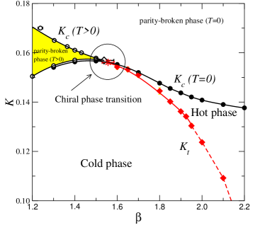
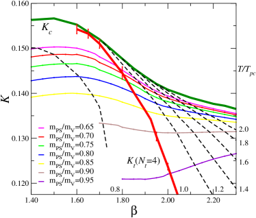
Figure 1: Left: Phase structure of QCD with Wilson-type quarks. Right: Lines of constant $m_{PS}/m_{V}$ and lines of constant $T/T_{pc}$.

We perform simulations for $N_{f}=2$ at $m_{PS}/m_{V}=0.80$. We adopt the Iwasaki (RG) improved gauge action and the clover improved Wilson fermion action:

$${\cal Z}(\beta,K,\mu) = \int{\cal D}U(\det M)^{N_{f}}e^{-S_{g}},\hskip 14.22636ptS_{g}=-\beta\left\{\sum_{x,\,\mu>\nu}c_{0}W_{\mu\nu}^{1\times 1}(x)+\sum_{x,\,\mu,\nu}c_{1}W_{\mu\nu}^{1\times 2}(x)\right\},$$

$$M_{x,y} = \delta_{x,y}-\delta_{x,y}c_{SW}K\sum_{\mu>\nu}\sigma_{\mu\nu}F_{\mu\nu}-K\sum_{i}\left[(1-\gamma_{i})U_{i}(x)~{}\delta_{x+\hat{i},y}+(1+\gamma_{i}){U_{i}}^{\dagger}(x-\hat{i})~{}\delta_{x-\hat{i},y}\right]$$ (1)

$$-K\left[e^{\mu}(1-\gamma_{4})U_{4}(x)~{}\delta_{x+\hat{4},y}-e^{-\mu}(1+\gamma_{4}){U_{4}}^{\dagger}(x-\hat{4})~{}\delta_{x-\hat{4},y}\right],$$

where $W_{\mu\nu}^{1\times 1}(x)$ and $W_{\mu\nu}^{1\times 2}(x)$ are $1\times 1$ and $1\times 2$ Wilson loops, $F_{\mu\nu}=(f_{\mu\nu}-f_{\mu\nu}^{\dagger})/(8i)$, $f_{\mu\nu}$ is the standard clover-shaped combination of gauge links, $\beta=6/g^{2}$, $c_{1}=-0.331$, $c_{0}=1-8c_{1}$, $c_{SW}=(1-0.8412\beta^{-1})^{-3/4}$, and $\mu\equiv\mu_{q}a$.

The phase structure of QCD at $\mu_{q}=0$ with this action has been investigated in Ref. [1]. The black line $(K_{c})$ in Fig. 1 (left) is the chiral limit, on which the pion mass vanishes at zero temperature. Above this line, a parity-flavor symmetry is spontaneously broken. Numerical simulations are performed in the normal phase below $K_{c}$. At finite temperature, the parity-flavor broken phase becomes narrow, that is the colored region in the upper left of Fig. 1 (left) for $N_{t}=4$. On the boundary of this phase, pion mass vanishes. The red line $(K_{t})$ is the finite temperature pseudo-critical line for $N_{t}=4$, separating the cold phase at small $\beta$ and the hot phase at large $\beta$.

The relation between the simulation parameters $(\beta,K)$ and the physical parameters is shown in Fig. 1 (right). We determine the lines of constant physics (LCP’s) by the mass ratio of pseudo-scalar meson and vector meson $m_{PS}/m_{V}$, interpolating the data of $m_{PS}$ and $m_{V}$ at $T=0$ in Refs. [1, 2, 3]. The temperature is estimated by the vector meson mass $m_{V}a$ using $T/m_{V}=1/(N_{t}m_{V}a)$, and normalized by $T_{pc}/m_{V}$, where $T_{pc}$ is the temperature at the pseudo-critical point on each LCP (see Sec.IV in Ref. [2]). Colored lines in Fig. 1 (right) are the lines of constant $m_{PS}/m_{V}$ (LCP’s) and dashed lines are the lines of constant $T/T_{pc}$. $(T/T_{pc}=0.8-2.0.)$ In this study, we generate 500 - 600 configurations (5000 - 6000 trajectories) for each simulation point. The lattice size is $N_{s}^{3}\times N_{t}=16^{3}\times 4$. The details of our simulations are given in Ref. [5].

3 Taylor expansion of the grand canonical potential

QCD at finite density is known to have a serious problem called “the sign problem”. To avoid this problem, we perform a Taylor expansion of physical quantities in terms of $\mu_{q}$ around $\mu_{q}=0$ and calculate the expansion coefficients, i.e. derivatives of the physical quantities, by numerical simulations at $\mu_{q}=0$, so that this calculation is free from the sign problem. The calculations of the derivatives are basic measurements in the study of QCD thermodynamics, since most of thermodynamic quantities are given by the derivatives of partition function ${\cal Z}(T,\mu_{u},\mu_{d})$, e.g., pressure $p$ and quark number density $n$ are defined by

$$\frac{p}{T^{4}}=\frac{1}{VT^{3}}\ln{\cal Z}\equiv\Omega,\hskip 22.76219pt\frac{n_{u(d)}}{T^{3}}=\frac{1}{VT^{3}}\frac{\partial\ln{\cal Z}}{\partial(\mu_{u(d)}/T)}=\frac{\partial(p/T^{4})}{\partial(\mu_{u(d)}/T)},$$ (2)

where $\mu_{u(d)}$ is the chemical potential for the u(d) quark. Quark number susceptibility $(\chi_{q})$ and isospin susceptibility $(\chi_{I})$ are given by

$$\frac{\chi_{q}}{T^{2}}=\left(\frac{\partial}{\partial(\mu_{u}/T)}+\frac{\partial}{\partial(\mu_{d}/T)}\right)\frac{n_{u}+n_{d}}{T^{3}},\hskip 14.22636pt\frac{\chi_{I}}{T^{2}}=\left(\frac{\partial}{\partial(\mu_{u}/T)}-\frac{\partial}{\partial(\mu_{d}/T)}\right)\frac{n_{u}-n_{d}}{T^{3}}.$$ (3)

Moreover the chiral condensate is defined by the derivative of $\ln{\cal Z}$ with respect to the quark mass.

We define the Taylor expansion coefficients of the pressure $p(T,\mu_{q})$ for the case $\mu_{u}=\mu_{d}\equiv\mu_{q}$ as

$$\frac{p}{T^{4}}=\sum_{n=0}^{\infty}c_{n}(T)\left(\frac{\mu_{q}}{T}\right)^{n},\hskip 22.76219ptc_{n}(T)=\frac{1}{n!}\frac{N_{t}^{3}}{N_{s}^{3}}\left.\frac{\partial^{n}\ln{\cal Z}}{\partial(\mu_{q}/T)^{n}}\right|_{\mu_{q}=0}.$$ (4)

The quark number and isospin susceptibilities for $\mu_{u}=\mu_{d}\equiv\mu_{q}$ are given by

$$\frac{\chi_{q}(T,\mu_{q})}{T^{2}}=2c_{2}+12c_{4}\left(\frac{\mu_{q}}{T}\right)^{2}+\cdots,\hskip 14.22636pt\frac{\chi_{I}(T,\mu_{q})}{T^{2}}=2c^{I}_{2}+12c^{I}_{4}\left(\frac{\mu_{q}}{T}\right)^{2}+\cdots,$$ (5)

where

$$c^{I}_{n}=\left.\frac{1}{n!}\frac{N_{t}^{3}}{N_{s}^{3}}\frac{\partial^{n}\ln{\cal Z}(T,\mu_{q}+\mu_{I},\mu_{q}-\mu_{I})}{\partial(\mu_{I}/T)^{2}\partial(\mu_{q}/T)^{n-2}}\right|_{\mu_{q}=0,\mu_{I}=0},\hskip 14.22636pt\mu_{I}=\frac{\mu_{u}-\mu_{d}}{2}.$$ (6)

The explicit forms of the coefficients are

$$c_{2}=\frac{N_{t}}{2N_{s}^{3}}{\cal A}_{2},\hskip 8.53581ptc_{4}=\frac{1}{4!N_{s}^{3}N_{t}}({\cal A}_{4}-3{\cal A}_{2}^{2}),\hskip 8.53581ptc_{2}^{I}=\frac{N_{t}}{2N_{s}^{3}}{\cal B}_{2},\hskip 8.53581ptc_{4}^{I}=\frac{1}{4!N_{s}^{3}N_{t}}({\cal B}_{4}-{\cal B}_{2}{\cal A}_{2}),$$ (7)

$${\cal A}_{2} = \left\langle{\cal D}_{2}\right\rangle+\left\langle{\cal D}_{1}^{2}\right\rangle,\hskip 14.22636pt{\cal A}_{4}=\left\langle{\cal D}_{4}\right\rangle+4\left\langle{\cal D}_{3}{\cal D}_{1}\right\rangle+3\left\langle{\cal D}_{2}^{2}\right\rangle+6\left\langle{\cal D}_{2}{\cal D}_{1}^{2}\right\rangle+\left\langle{\cal D}_{1}^{4}\right\rangle,$$

$${\cal B}_{2} = \left\langle{\cal D}_{2}\right\rangle,\hskip 14.22636pt{\cal B}_{4}=\left\langle{\cal D}_{4}\right\rangle+2\left\langle{\cal D}_{3}{\cal D}_{1}\right\rangle+\left\langle{\cal D}_{2}^{2}\right\rangle+\left\langle{\cal D}_{2}{\cal D}_{1}^{2}\right\rangle,$$ (8)

where ${\cal D}_{n}=N_{f}[\partial^{n}\ln\det M/\partial\mu^{n}]$ and $\mu\equiv\mu_{q}a$.
${\cal D}_{1}=N_{f}{\rm tr}[(\partial M/\partial\mu)M^{-1}],\hskip 2.84526pt{\cal D}_{2}=N_{f}[{\rm tr}[(\partial^{2}M/\partial\mu^{2})M^{-1}]-{\rm tr}[(\partial M/\partial\mu)M^{-1}(\partial M/\partial\mu)M^{-1}]],\ldots$
The derivative of the fermion matrix $M$ at $\mu=0$ is

$$\frac{\partial^{n}M}{\partial\mu^{n}}=\left\{\begin{array}[]{l}-K\left((1-\gamma_{4})U_{4}(x)~{}\delta_{x+\hat{4},y}-(1+\gamma_{4}){U_{4}}^{\dagger}(x-\hat{4})~{}\delta_{x-\hat{4},y}\right)\ \ {\rm for}\ n:{\rm odd.}\\ -K\left((1-\gamma_{4})U_{4}(x)~{}\delta_{x+\hat{4},y}+(1+\gamma_{4}){U_{4}}^{\dagger}(x-\hat{4})~{}\delta_{x-\hat{4},y}\right)\ \ {\rm for}\ n:{\rm even.}\end{array}\right.$$ (11)

For the calculation of these operators, the random noise method is used. We generate $N_{noise}$ of U(1) noise vectors $\left(\eta_{i,\alpha}\right)_{x,\beta}\equiv\eta(i,x)\delta_{\alpha,\beta}$, where $\eta(i,x)$ is a U(1) random number $(\eta=e^{i\theta};0\leq\theta<2\pi)$ which satisfies $(1/N)\sum_{i=1}^{N}\eta(i,x)\eta^{*}(i,y)=\delta_{x,y}$ for large $N$. $\alpha=1,\cdots,12$ is the color and spinor index. Then $\lim_{N\to\infty}(1/N)\sum_{i=1}^{N}\sum_{\alpha=1}^{12}\left(\eta_{i,\alpha}\right)_{x,\beta}\left(\eta_{i,\alpha}^{*}\right)_{y,\gamma}=\delta_{x,y}\delta_{\beta,\gamma}$, hence

$${\rm tr}\left(\frac{\partial^{n}M}{\partial\mu^{n}}M^{-1}\cdots M^{-1}\right) \approx \frac{1}{N_{noise}}\sum_{i=1}^{N_{noise}}\sum_{\alpha=1}^{12}\eta_{i,\alpha}^{\dagger}\frac{\partial^{n}M}{\partial\mu^{n}}X_{i,\alpha},\hskip 28.45274pt(n=1,2,\cdots),$$ (12)

where $X_{i,\alpha}$ is the solution of $MX_{i,\alpha}=(\cdots M^{-1})\eta_{i,\alpha}$.

4 Quark number and isospin susceptibilities

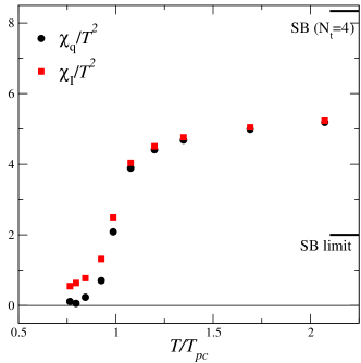
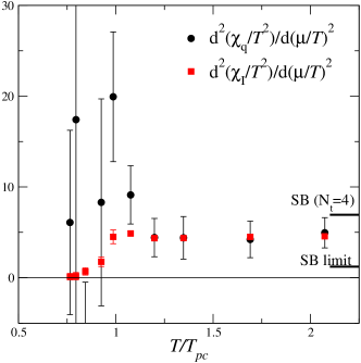
Figure 2: Left: Quark number (black) and isospin (red) susceptibilities. Right: The second derivatives of these susceptibilities.

We calculate the expansion coefficients $c_{2},c_{4},c_{2}^{I}$ and $c_{4}^{I}$. The black and red symbols in Fig. 2 (left) are the quark number susceptibility $\chi_{q}/T^{2}=2c_{2}$ and isospin susceptibility $\chi_{I}/T^{2}=2c_{2}^{I}$, respectively. We also plot preliminary results of the second derivatives of these susceptibilities $\partial^{2}(\chi_{q}/T^{2})/\partial(\mu_{q}/T)^{2}=24c_{4}$ (black symbols) and $\partial^{2}(\chi_{I}/T^{2})/\partial(\mu_{q}/T)^{2}=24c_{4}^{I}$ (red symbols) in Fig. 2 (right). In this study, we choose $N_{noise}=10$ for the calculations of the operators in Eq. (8) except for the operators ${\rm tr}[(\partial^{n}M/\partial\mu^{n})M^{-1}]$, where $n=1-4$. We increase the number of noise vectors up to $N_{noise}=50$ for ${\rm tr}[(\partial^{n}M/\partial\mu^{n})M^{-1}]$ to efficiently reduce statistical errors. (See discussions below.)

To check the reliability of the random noise method, we calculate the operators ${\cal D}_{n}$ $(n=1-4)$ using two independent sets of noise vectors with $N_{noise}=10$ on the same configurations . Figure 3 (left) shows the time history of the imaginary part of ${\cal D}_{1}$ and the real part of ${\cal D}_{2}$ computed by two series of noise sets. The operator ${\cal D}_{n}$ is real for $n$ even and purely imaginary for $n$ odd, and the expectation value of ${\cal D}_{1}$ is zero because an expectation value of imaginary part is always zero at $\mu_{q}=0$ [6]. It is found that two results of ${\cal D}_{2}$ obtained by different noise sets are consistent with each other on each configuration, while two results of ${\cal D}_{1}$ are sensibly different. This means that errors from the noise method is dominating in ${\cal D}_{1}$ with $N_{noise}=10$. Moreover we found that the error from ${\cal D}_{1}$ dominates in $c_{4}$ and $c_{4}^{I}$ through Eq. (8). Therefore, in reducing the errors for second derivatives, it is efficient to increase $N_{noise}$ for ${\cal D}_{1}$, keeping $N_{noise}=10$ for other operators.

As seen in Fig. 2 (left), $\chi_{q}/T^{2}$ and $\chi_{I}/T^{2}$ increase sharply at $T_{pc}$, in accordance with the expectation that the fluctuations in the quark-gluon plasma phase are much larger than those in the hadron phase. These results agree qualitatively with previous results by staggered-type quarks [4, 7]. Moreover the result of $\partial^{2}(\chi_{I}/T^{2})/\partial(\mu_{q}/T)^{2}$ is quite similar to the results by p4-improved staggered fermions [4]. This suggests that there are no singularities in $\chi_{I}$ at non-zero density, as discussed in Ref. [4]. On the other hand, we expect a large enhancement in the quark number fluctuations near $T_{pc}$ as approaching the critical endpoint in the $(T,\mu_{q})$ plane. Although the results in Fig. 2 (right) have large statistical errors, the results of $\partial^{2}(\chi_{q}/T^{2})/\partial(\mu_{q}/T)^{2}$ near $T_{pc}$ show quite different behavior from those of $\chi_{I}$. The second derivative of $\chi_{q}$ near $T_{pc}$ seems to be more than three times larger than those at high temperature, suggesting the large fluctuations near the critical point. However, the lattice discretization error in the equation of state is known to be large for the action in Eq. (1). The short lines in the right end denote the values in the free quark-gluon gas (Stefan-Boltzmann) limit, both for $N_{t}=4$ and in the continuum. It is clear that we need further studies increasing the statistics and decreasing the lattice spacing.

5 Lines of constant pressure

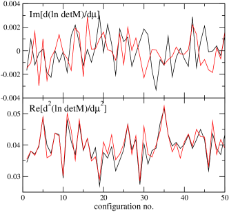
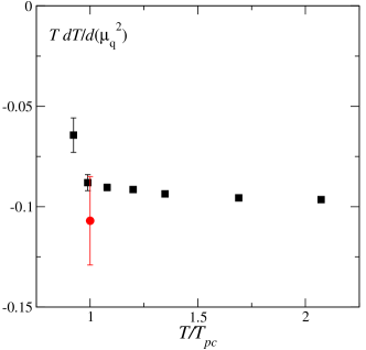
Figure 3: Left: Time history of ${\cal D}_{1}$ (top) and ${\cal D}_{2}$ (bottom) obtained by different noise sets at $T/T_{pc}=0.925,m_{PS}/m_{V}=0.8$. Right: Slope of the line of constant pressure at $\mu_{q}=0$.

It is interesting to compare the line of constant pressure (and energy density) with $T_{pc}(\mu_{q})$ and the chemical freeze out points [8]. Here we consider the pressure constant line in the $(T,\mu_{q}^{2})$ plane,

$$\Delta p=\frac{\partial p}{\partial T}\Delta T+\frac{\partial p}{\partial(\mu_{q}^{2})}\Delta(\mu_{q}^{2})=\left[T^{4}\frac{\partial(p/T^{4})}{\partial T}+\frac{4p}{T}\right]\Delta T+\left[T^{4}\frac{\partial(p/T^{4})}{\partial(\mu_{q}^{2})}\right]\Delta(\mu_{q}^{2})=0.$$ (13)

From this equation, the slope of the $p$-constant line at $\mu_{q}=0$ is given by

$$T\frac{{\rm d}T}{{\rm d}(\mu_{q}/T)^{2}}=\left.-\frac{\partial(p/T^{4})}{\partial(\mu_{q}/T)^{2}}\right/\left(T\frac{\partial(p/T^{4})}{\partial T}+\frac{4p}{T^{4}}\right).$$ (14)

Using the data of $\partial(p/T^{4})/\partial(\mu_{q}/T)^{2}=\chi_{q}/T^{2}$ in Fig. 2, $p/T^{4}$ and $T\partial(p/T^{4})/\partial T$ in Ref. [2], we estimate the slope of the line of constant pressure at $\mu_{q}=0$. The results at $m_{PS}/m_{V}=0.8$ are shown in Fig. 3 (right). The slope at $\mu_{q}=0$ is about $-0.1$. This is roughly consistent with the previous results by p4-improved staggered fermions at $m_{PS}/m_{V}=0.7$ in Ref. [6], which is denoted by the red dot. Moreover the slope of the phase transition line in Ref. [6] is $T{\rm d}T_{pc}/{\rm d}(\mu_{q}/T)^{2}\approx-0.07(3)$. The line of constant $p$ is almost parallel to the phase transition line. On the other hand, the slope $T{\rm d}T/{\rm d}(\mu_{q}/T)^{2}$ of the line of the chemical freeze out in the $(T,\mu_{q}^{2})$ plane are about $-0.25$ [8]. Further studies at small quark mass and large $N_{t}$ are necessary to compare with experimental results.

6 Conclusion

We reported the current status of our study of QCD thermodynamics with a Wilson-type quark action. The lines of constant physics in the $(\beta,K)$ plane as well as the relation between the parameters $(\beta,K)$ and $(T/T_{pc},m_{PS}/m_{V})$ are determined. Simulations are performed on a $16^{3}\times 4$ lattice. The derivatives of pressure with respect to $\mu_{q}$ and $\mu_{I}$ up to 4th order are computed. The random noise method is used. For the calculation of 4th order derivatives, the choice of the number of noise vector $(N_{noise})$ is important. We discussed the fluctuations of quark number and isospin densities. Although the statistical errors are still large, a clear quantitative difference between the second derivatives of $\chi_{q}$ and $\chi_{I}$ is observed. $\chi_{q}$ seems to increase rapidly near $T_{pc}$ as $\mu_{q}$ increases, whereas the increase of $\chi_{I}$ is not large near $T_{pc}$. These behaviors agree with the results obtained by p4-improved staggered fermions qualitatively, and with the expectation from the sigma model.

Acknowledgements:

This work is in part supported by Grants-in-Aid of the Japanese Ministry of Education, Culture, Sports, Science and Technology, (Nos. 13135204, 15540251, 17340066, 18540253, 18740134). SE is supported by the Sumitomo Foundation (No. 050408), and YM is supported by JSPS. This work is in part supported also by the Large-Scale Numerical Simulation Projects of ACCC, Univ. of Tsukuba, and by the Large Scal Simulation Program of High Energy Accelerator Research Organization (KEK).

References

- [1] A. Ali Khan et al. (CP-PACS Collaboration), Phase structure and critical temperature of two-flavor QCD with renormalization group improved gauge action and clover improved Wilson quark action, Phys. Rev. D63 (2001) 034502 [hep-lat/0008011]
- [2] A. Ali Khan et al. (CP-PACS Collaboration), Equation of state in finite-temperature QCD with two flavors of improved Wilson quarks, Phys. Rev. D64 (2001) 074510 [hep-lat/0103028].
- [3] A. Ali Khan et al. (CP-PACS Collaboration), Light Hadron Spectroscopy with Two Flavors of Dynamical Quarks on the Lattice, Phys. Rev. D65 (2002) 054505 [hep-lat/0105015]
- [4] C.R. Allton, S. Ejiri, S.J. Hands, O. Kaczmarek, F. Karsch, E. Laermann and C. Schmidt, The Equation of State for Two Flavor QCD at Non-zero Chemical Potential, Phys. Rev. D68 (2003) 014507 [hep-lat/0305007]; C.R. Allton, M. Döring, S. Ejiri, S.J. Hands, O. Kaczmarek, F. Karsch, E. Laermann and K. Redlich, Thermodynamics of two flavor QCD to sixth order in quark chemical potential, Phys. Rev. D71 (2005) 054508 [hep-lat/0501030].
- [5] N. Ukita, S. Ejiri, T. Hatsuda, N. Ishii, Y. Maezawa, S. Aoki and K. Kanaya, Finite temperature phase transition of two-flavor QCD with an improved Wilson quark action, in proceedings of Lattice 2006. \posPoS(LAT2006)150.
- [6] C.R. Allton, S. Ejiri, S.J. Hands, O. Kaczmarek, F. Karsch, E. Laermann, Ch. Schmidt and L. Scorzato, The QCD thermal phase transition in the presence of a small chemical potential, Phys. Rev. D66 (2002) 074507 [hep-lat/0204010].
- [7] S. Gottlieb, W. Liu, D. Toussaint, R.L. Renken and R.L. Sugar, Fermion Number Susceptibility In Lattice Gauge Theory, Phys. Rev. D38 (1988) 2888.
- [8] P. Braun-Munzinger, K. Redlich and J. Stachel, Particle Production in Heavy Ion Collisions, in Quark Gluon Plasma 3 (World Scientific Publishing, 2003) [nucl-th/0304013].