SWAT/06/466

September 2006

Chiral Symmetry Restoration

in Anisotropic QED₃

Iorwerth Owain Thomas^a and Simon Hands^b

^aDepartment of Physics, Loughborough University,

Loughborough, Leicestershire LE11 3TU, U.K.

^bDepartment of Physics, Swansea University,

Singleton Park, Swansea SA2 8PP, U.K.

Abstract

We present results from a Monte Carlo simulation of non-compact lattice QED in 3 dimensions in which an explicit anisotropy $\kappa$ between $x$ and $y$ hopping terms has been introduced into the action. Using a parameter set corresponding to broken chiral symmetry in the isotropic limit $\kappa=1$, we study the chiral condensate on $16^{3}$, $20^{3}$, and $24^{3}$ lattices as $\kappa$ is varied, and fit the data to an equation of state which incorporates anisotropic volume corrections. The value $\kappa_{c}$ at which chiral symmetry is apparently restored is strongly volume-dependent, suggesting that the transition may be a crossover rather than a true phase transition. In addition we present results on $16^{3}$ lattices for the scalar meson propagator, and for the Landau gauge-fixed fermion propagator. The scalar mass approaches the pion mass at large $\kappa$, consistent with chiral symmetry restoration, but the fermion remains massive at all values of $\kappa$ studied, suggesting that strong infra-red fluctuations persist into the chirally symmetric regime. Implications for models of high-$T_{c}$ superconductivity based on anisotropic QED₃ are discussed.

PACS: 11.10.Kk, 11.15.Ha, 71.27.+a, 74.25.Dw

Keywords: lattice gauge theory, cuprate, phase diagram, pseudogap

1 Introduction

QED₃  , i.e. quantum electrodynamics restricted to two dimensions of space and one of time, has recently been the focus of some attention in the condensed matter community, as various versions of it are examined as candidate effective models of high-temperature superconductivity in cuprate compounds.

The particular model in which we are interested is that presented in [1, 2], which is supposed to model the passage between the antiferromagnetic SDW (spin-density wave) and superconducting dSC (the d denotes the superconducting order parameter has $d$-wave symmetry) phases at low temperature $T$ as the doping fraction $x$ is increased. QED₃ is proposed, as reviewed below in Sec. 2.1, as an effective theory of the low-energy quasiparticle excitations in the neighbourhood of the 4 nodes in the gap function $\Delta(\vec{k})$. Since the dispersion relation is linear at the nodes, the excitations can be reinterpreted as various components of a relativistic spinor field $\Psi$ with 4 spin and $N_{f}=2$ flavour degrees of freedom. Interaction via a minimally-coupled abelian vector gauge potential field $A_{\mu}$ arises as a result of phase fluctuations of $\Delta$; it can then be argued that $A_{\mu}$ is most naturally governed by an action of a Maxwell type [1, 2], resulting in massless photon degrees of freedom which have an alternative interpretation as the Goldstone bosons associated with the condensation of dual vortices [3, 4].

QED₃ is a quantum field theory whose study has a long history (see [5] for a brief review). The main issue is chiral symmetry breaking ($\chi$SB), i.e. whether chiral symmetry, the invariance of the action under independent global rotations of left- and right-handed helicity spinors, is spontaneously broken, signalled by a chiral condensate $\langle\bar{\Psi}\Psi\rangle\not=0$. $\chi$SB implies dynamical mass generation, i.e. the physical fermion mass $M$ may be much greater than the “bare” or Lagrangian mass $m$. This is believed to depend sensitively on the number of fermion species $N_{f}$ in the model; $\chi$SB is supposed to occur only for $N_{f}$ less than some critical $N_{fc}$, whose precise value remains a goal of non-perturbative quantum field theory.

In the condensed-matter context, the $\chi$SB order parameter can be mapped directly into the SDW one. If $\chi$SB does not occur (i.e. $N_{f}>N_{fc}$), then the resulting theory of light fermion degrees of freedom interacting with massless gauge degrees of freedom is proposed as a theory of the so-called “pseudogap” region of the cuprate phase diagram, characterised by spectral depletion in the immediate vicinity of the Fermi energy even in the absence of a well-defined quasiparticle peak. The main prediction of the QED₃ approach is thus that if $N_{fc}>2$ the dSC and SDW phases are connected in the $T\to 0$ limit [2], whereas if $N_{fc}<2$ they are separated by a region of pseudogap phase [1].

An important assumption in the above chain of reasoning is that results from continuum QED₃ in the isotropic limit (as usually studied in quantum field theory) can be applied directly to the condensed-matter system, whose Lagrangian density (LABEL:eq:finalbit) below has kinetic terms describing a single flavour with differing strengths or “velocities” in $x$- and $y$-directions as an artifact of the transformation to the relativistic spinor basis. This is in principle not a negligible effect; the velocity ratio or anisotropy $\kappa$ in real cuprates varies with $x$ [6], and can be as large as 7 at the onset of the dSC phase [7]. Evidence in favour of applying predictions of the isotropic theory comes from a renormalisation-group analysis, which studied small anisotropy perturbations to the isotropic system and concluded that weak anisotropy is an irrelevant perturbation [8, 9]. This result is then used to argue that the critical $N_{fc}$ is a universal constant, independent of $\kappa$, and hence that the various estimates of $N_{fc}$ in the literature can be applied to the cuprate problem.

It should be noted here that similar ideas regarding relativistic fermions (often four-Fermi theories) have been also been discussed in the literature relating to graphene and similar compounds, both theoretically (for example, see [10, 11, 12, 13]) and experimentally (for example [14]). However, this form has only an asymmetry between temporal and spatial directions, whereas in what follows we treat a more generally anisotropic system where all three Euclidean axes are distinguished.

In our previous paper [15] we made the first study of anisotropic QED₃ using the methods of numerical lattice gauge theory, a non-perturbative technique with very different systematic approximations to continuum-based approaches. Using a large value of the fermion-photon coupling strength, we studied the $\chi$SB order parameter $\langle\bar{\chi}\chi\rangle$ on a relatively modest $16^{3}$ spacetime lattice as the anisotropy $\kappa$ is increased from 1, and provided preliminary results that suggest the existence of a chiral symmetry restoring phase transition at a critical value $\kappa_{c}$; moreover, we found that the “renormalised” $\kappa_{R}$ – obtained by considering the spatial decay of correlations of pseudoscalar meson or “pion” fermion – anti-fermion ($f\bar{f}$) bound states – obeyed $\kappa_{R}>\kappa$, suggesting in contrast to [8] that $\kappa$ is in fact a relevant parameter. Both observations suggest caution should be used in applying isotropic QED₃ directly to cuprates.

Several questions raised by [15] are addressed in the current paper. Firstly, we wish to understand the nature of the chiral symmetry restoring transition, using the traditional method of studying the transition on larger systems and applying a finite-volume scaling analysis. New results on $20^{3}$ and $24^{3}$ lattices, together with analyses assuming both isotropic and weakly anisotropic finite volume scaling are presented in Sec. 3. As we shall see, the data is best fitted by an ansatz which takes anisotropy into account, which suggests that the value of $\kappa_{c}$ in the thermodynamic limit may be considerably larger than the estimate $\kappa_{c}\simeq 4.5$ of [15]. Next, in Sec. 4 we have studied spectroscopy in another $f\bar{f}$ channel with scalar, rather than pseudoscalar, quantum numbers. This is important for two reasons. Firstly, as the parity partner of the pseudoscalar the scalar should become degenerate with the pion at large $\kappa$, giving further evidence for the restoration of chiral symmetry. Secondly, since the pion is the Goldstone boson associated with $\chi$SB in the low-$\kappa$ phase, it is in some sense a “distinguished particle”, and motivates us to check the renormalised anisotropy $\kappa_{R}$ using a different channel.

Finally, for the first time we present results for the fermion propagator $\langle\chi(x)\bar{\chi}(y)\rangle$. Since this is not a gauge invariant object, in order to obtain a non-zero result this has necessitated the implementation of a gauge fixing procedure, described in some detail in Sec. 5.1. Our motivation comes from the arguments of Tešanović et al. [1, 16], suggesting that the massless quasiparticles of the pseudogap phase acquire a small, gauge dependent anomalous dimension due to their interaction with the statistical gauge field, which may explain non-standard scaling of transport coefficients such as resistivity and thermal conductivity in the pseudogap phase. From a numerical point of view this has proved easily the most demanding part of the project, requiring much computational effort to extract any kind of signal from the statistical noise inherent in the Monte Carlo method. Somewhat unexpectedly, we find evidence for the persistence of a dynamically generated fermion mass in the high-$\kappa$ phase, despite the apparent restoration of chiral symmetry. A physical scenario consistent with these observations is discussed further in Sec. 6.

2 Review of the Lattice Model

2.1 QED₃ as an effective theory of the pseudogap

The mapping of the pseudogap region of the cuprate phase diagram onto QED₃ is derived in detail in [1, 2], and reviewed in language more accessible to particle physicists in [15]. Here we briefly summarise, starting with the following Euclidean (imaginary time) action, also known as the Bogoliubov – deGennes model, for $d$-wave quasiparticles in the dSC phase.

$$S = T\sum_{\vec{k},\sigma,\omega_{n}}\biggl{[}(i\omega_{n}-\xi_{\vec{k}})c^{\dagger}_{\sigma}(\vec{k},\omega_{n})c_{\sigma}(\vec{k},\omega_{n})$$ (1)

$$- {\sigma\over 2}\left(\Delta(\vec{k})c^{\dagger}_{\sigma}(\vec{k},\omega_{n})c^{\dagger}_{-\sigma}(-\vec{k},-\omega_{n})-\Delta^{\dagger}(\vec{k})c_{\sigma}(\vec{k},\omega_{n})c_{-\sigma}(-\vec{k},-\omega_{n})\right)\biggr{]},$$

where $c^{\dagger},c$ are creation and annihilation operators for electrons with spin $\sigma=\pm 1$, $\omega_{n}=(2n-1)\pi T$ are the allowed Matsubara frequencies, the function $\xi_{\vec{k}}$ is the energy of a free quasiparticle (which thus vanishes for $\vec{k}$ on the Fermi surface), and $\Delta(\vec{k})$ is the gap function, which can be thought of as a self-consistent pairing field. Due to its $d$-wave symmetry, $\Delta$ actually vanishes at two pairs of node momenta $\vec{k}=\pm\vec{K}_{1},\pm\vec{K}_{2}$, with $\vec{K}_{1}.\vec{K}_{2}=0$.

Linearising the latter functions around the nodes and defining the 4-spinor $\Psi_{i}$ at the node pair $i$ as

$$\Psi_{i}^{\mbox{tr}}(\vec{q},\omega)=\left(c_{+}(\vec{k},\omega),c^{\dagger}_{-}(-\vec{k},-\omega),c_{+}(\vec{k}-2\vec{K}_{i},\omega),c^{\dagger}_{-}(-\vec{k}+2\vec{K}_{i},-\omega)\right),$$ (2)

we may write the following effective action describing the behaviour of the system at low $T$ [8]:

$$S=\int d^{2}r\int_{0}^{\beta}d\tau\bar{\Psi}_{1}[\gamma_{0}D_{\tau} + \delta\kappa^{-\frac{1}{2}}\gamma_{1}D_{x}+\delta\kappa^{\frac{1}{2}}\gamma_{2}D_{y}]\Psi_{1}+$$

$$\bar{\Psi}_{2}[\gamma_{0}D_{\tau} + \delta\kappa^{-\frac{1}{2}}\gamma_{1}D_{y}+\delta\kappa^{\frac{1}{2}}\gamma_{2}D_{x}]\Psi_{2}+\frac{1}{2g^{2}}F_{\mu\nu}^{2},$$

where $\beta\equiv 1/T$, $\kappa=v_{F}/v_{\Delta}$ (where $v_{F}$ and $v_{\Delta}$ are the Fermi and Gap velocities derived from the linearisation of $\xi_{\vec{k}}$ and $\Delta(\vec{k})$ respectively about the nodes) is the anisotropy, $\delta=\sqrt{v_{F}v_{\Delta}}$, and the $4\times 4$ traceless hermitian matrices $\gamma_{\mu}$ obey $\{\gamma_{\mu},\gamma_{\nu}\}=2\delta_{\mu\nu}$. The action (LABEL:eq:finalbit) describes $N_{f}=2$ flavours of relativistic fermion $\Psi$ (sometimes known as ‘nodal fermions’ in this context) interacting with an abelian gauge potential $A_{\mu}$, which we will often refer to as the ‘photon’, via the covariant derivative $D_{\mu}\equiv\partial_{\mu}+iA_{\mu}$. The photon-fermion interaction models the effect of the phase fluctuations of the pairing field $\Delta$: photon dynamics are governed by $F_{\mu\nu}^{2}\equiv(\partial_{[\mu}A_{\nu]})^{2}$, and the coupling $g$ (the analogue of ‘electron charge’ in textbook QED) is related to the diamagnetic susceptibility $\chi$ via $g\sim\chi^{-{1\over 2}}$ [1].

The two velocities depend on the shape of the Fermi surface, and hence on the doping of the superconductor [6, 7], implying that the same is true of $\kappa$; at the onset of superconductivity at low $T$ $\kappa$ may be as much as $O(7)$.

2.2 Lattice Model of Anisotropic QED₃

The formulation of isotropic QED₃  on a spacetime lattice is described in detail in [17]; in what follows we summarise the treatment of our anisotropic model given in [15]. For $N$ flavours of staggered lattice fermion, the following is a QED₃  action with an explicit spatial anisotropy:

$$S=\sum_{i=1}^{N}\sum_{x,x^{\prime}}a^{3}\bar{\chi_{i}}(x)M_{x,x^{\prime}}\chi_{i}(x^{\prime})+\frac{\beta}{2}\!\!\sum_{x,\mu<\nu}\!\!a^{3}\Theta_{\mu\nu}^{2}(x).$$ (4)

We define the fermion matrix $M_{x,x^{\prime}}$ as follows:

$$M_{x,x^{\prime}}={1\over 2a}\sum_{\mu=1}^{3}\xi_{\mu}(x)[\delta_{x^{\prime},x+\hat{\mu}}U_{x\mu}-\delta_{x^{\prime},x-\hat{\mu}}U_{x^{\prime}\mu}^{\dagger}]+m\delta_{\mu\nu}$$ (5)

where $\xi_{\mu}$ is

$$\xi_{\mu}(x)=\lambda_{\mu}\eta_{\mu}(x)$$ (6)

and $\eta_{\mu}(x)=(-1)^{x_{1}+...+x_{\mu-1}}$, where $x_{1}=x$, $x_{2}=y$ and $x_{3}=\tau$, is the Kawomoto-Smit phase of the staggered fermion field. The physical lattice spacing is denoted by $a$. The $\lambda_{\mu}$ are anisotropy factors, which we define like so: $\lambda_{x}=\kappa^{-\frac{1}{2}}$, $\lambda_{y}=\kappa^{\frac{1}{2}}$, $\lambda_{t}=1$. The $\eta$ factors ensure that the action describes relativistic covariant fermions in the isotropic limit $\kappa=1$.

Taking the photon-like degree of freedom $\theta_{\mu}(x)$ to exist on the link connecting site $x$ to site $x+\hat{\mu}$, makes $U_{\mu}(x)\equiv\exp(ia\theta_{\mu}(x))$ in (5) the parallel transporter defining the gauge interaction with the fermions; we may define a non-compact gauge action via

$$\Theta_{\mu\nu}(x)={1\over a^{2}}[\Delta_{\mu}^{+}\theta_{\nu}(x)-\Delta_{\nu}^{+}\theta_{\mu}(x)].$$ (7)

The dimensionless parameter $\beta$ is given in terms of the QED coupling constant via $\beta\equiv 1/g^{2}a$. It is convenient to work wherever possible in ‘lattice units’ such that $a=1$.

It is important that a distinction is made between our particular use of anisotropy, which treats it as a physical property of the system that can be observed and renormalised through quantum corrections, and the more general use of anisotropic cutoffs in lattice field theory, wherein the anisotropies are controlled such that they disappear in the continuum limit, maintaining the Lorentz covariance of the theory. In this latter case, anisotropy is not physically observable.

2.3 The Simulation

In Reference [15] we simulated the dynamics of the lattice action (4,5) using a hybrid Monte Carlo algorithm on a $16^{3}$ lattice for $\kappa$ ranging from 1 to 10 and the bare mass $m=0.05,\ldots,0.01$. The gauge coupling constant $\beta$ was held at a constant value 0.2 throughout – at this relatively strong coupling the system is in a state of spontaneously broken chiral symmetry at $\kappa=1$. The main results of [15] are that the chiral condensate decreases with increasing $\kappa$, consistent with a second order chiral symmetry restoring transition at $\kappa_{c}=4.35(2)$, and that the renormalised anisotropy $\kappa_{R}$ obtained by comparison of pion correlators in $x$- and $y$-directions obeys

$$\kappa_{R}-1\approx 2(\kappa-1),$$ (8)

implying that $\kappa$ is a relevant parameter.

In the calculations presented in this paper, unless otherwise noted, the gauge configuration ensemble $\{\theta\}$ used was generated using the same Hybrid Monte Carlo algorithm, running for around 1000 trajectories of mean length 1.0 on $L^{3}$ lattices with $L=16$, and the gauge coupling set to the same value $\beta=0.2$. Even-odd partitioning was used; this allowed us to set $N=1$, giving us $N_{f}=2$ in the continuum limit. Typical acceptances were $60-70\%$ for $m=0.01$, and $70-80\%$ for other bare mass values.

A novelty of this paper is that we have extended our study to a range of volumes: datasets for the $20^{3}$ and $24^{3}$ lattices typically contain 700 and 600-700 trajectories per point with acceptances of $82-94\%$ and $75-82\%$ respectively. In the the studies of fermion propagation presented in Sec. 5, gauge-fixed configurations were generated on a $16^{3}$ lattice and consisted of $\sim$30,000 trajectories per point with an acceptance rate of $79-87\%$.

3 Susceptibilities and Finite Size Scaling

We begin the presentation of our results with measurements of longitudinal susceptibility and the chiral condensate as $L$ is varied. This is necessary to pin down the nature of the chiral symmetry restoring transition with more precision. Apart from the intrinsic theoretical interest, there are important phenomenological issues at stake. Firstly, it is important to know the value of the critical anisotropy $\kappa_{c}$ at which the transition takes place in the continuum and thermodynamic limits, since in principle this is a physically observable parameter in real cuprates [6]. Secondly, the order of the phase transition is important; were it either first-order or a crossover, then an immeasurably small but non-vanishing condensate may persist in the high-$\kappa$ “chirally restored phase”, meaning that antiferromagnetic order can survive the transition [15]. As we shall see below, the results we have been able to obtain with our resources have not settled the issue unequivocally; it seems likely that a model of finite volume scaling which takes account of the anisotropy is required.

3.1 Finite size scaling of the condensate

Here we present the results of a preliminary study of the finite size scaling of the chiral condensate and longitudinal susceptibility at fermion mass $m=0.01$, the smallest of the bare masses examined in [15]. We define the chiral condensate in terms of the trace of the inverse of the fermion matrix $M$:

$$\langle\bar{\chi}\chi\rangle=-{1\over V}{{\partial\ln Z}\over\partial m}={1\over V}\langle\mbox{tr}M^{-1}\rangle,$$ (9)

and the longitudinal susceptibility in terms of its derivative,

$$\chi_{l}=\frac{\partial\langle\bar{\chi}\chi\rangle}{\partial m}={1\over V}[\langle(\mbox{tr}M^{-1})(\mbox{tr}M^{-1})\rangle-\langle\mbox{tr}M^{-1}\rangle^{2}-\langle\mbox{tr}(M^{-1}M^{-1})\rangle].$$ (10)

Note that eqn. (10) includes diagrams which are both connected and disconnected in terms of fermion lines; both contributions were calculated.

In the vicinity of the phase transition $\chi_{l}$ should peak at an anisotropy $\kappa_{peak}$ which should tend towards the critical value $\kappa_{c}$ in the thermodynamic limit. Examining the plot of the longitudinal susceptibility as the size of the lattice is varied (Figure 1), we observe that the peak shifts to the right by an amount that decreases as the lattice size increases; this suggests that a second order transition might occur at a finite value of $\kappa_{c}$ in the thermodynamic limit. Unexpectedly, however, the magnitude of the peak appears suppressed as the lattice size increases. This may have several possible causes:

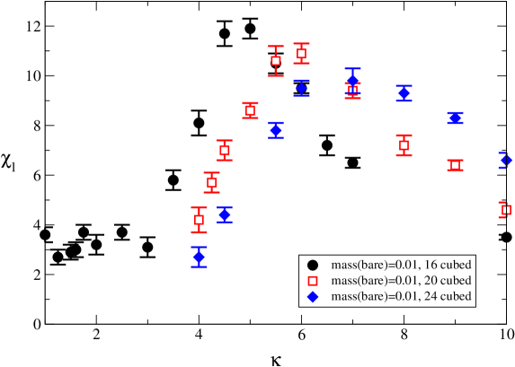
Figure 1: $\chi_{l}$ for various lattice sizes and $m=0.01$.

• The magnitude of the peak does increase, but the width of the peak as the lattice volume increases narrows such that it falls between the available data points and is not detected. The rounded shape of the curves suggests that this is unlikely.

• This is not a second order phase transition; perhaps we’re observing a crossover instead. If there is a crossover between the two phases, and not a genuine second-order phase transition, then a small chiral condensate is expected to persist in the high-$\kappa$ phase. Some analytic approaches predict dimensionless condensates $\beta^{2}\langle\bar{\chi}\chi\rangle$ as small as $O(10^{-4})$ [18]. Attempts to rule out this possibility regarding the chiral phase transition in studies of isotropic QED₃  with various $N_{f}$ such as [17, 5] have not proven to be successful, and it is also likely to be as difficult in this case.

• Our system has an anisotropic coupling between the gauge and fermion fields. The effects of this could be difficult to account for in the standard finite size scaling developed for phase transitions in isotropic systems; we should turn our attention to the scaling of anisotropic systems instead. In the statistical mechanics literature, one observes two models of this scaling:

  • Weak anisotropy: In these systems, there exist different correlation lengths in different directions; these correlation lengths can be rescaled such that the system is effectively isotropic in the scaling region ([19] and references therein, notably [20, 21, 22]). We examine this possibility in detail below.

  • Strong anisotropy: In these systems in addition to correlation lengths, the critical exponent $\nu$ is different in different directions ([22, 23] and references therein). The scaling behaviour of these systems is very sensitive to the shape of the lattice, and is difficult to treat with data generated on cubic lattices; it is mentioned here as an issue worthy of further investigation.

Since our data is restricted to that generated on a square lattice, we will examine only weak anisotropic scaling as compared to isotropic scaling.

3.1.1 Isotropic scaling

Firstly, we shall discuss the scaling of the system if it is assumed intrinsically isotropic. As argued in [24], we can use the scaling behaviour of the system as we vary $L$ in order to determine how the finite volume affects the equation of state. We do this by treating the inverse linear size of the lattice, $L^{-1}$, as an irrelevant scaling field and use the following as our ansatz, where $k=(\kappa-\kappa_{c})$:

$$m=B\langle\bar{\chi}\chi\rangle^{\delta}+A(k+CL^{-1/\nu})\langle\bar{\chi}\chi\rangle^{\rho}.$$ (11)

Here $\delta$, $\nu$ and $\beta\equiv(\delta-\rho)^{-1}$ have their usual meanings as critical indices describing a continuous phase transition.

3.1.2 Weakly anisotropic scaling

In this case, we wish to account for the distortion of the correlation lengths of the system along the $x$ and $y$ axes by $\kappa\neq 1$. Finite size effects enter into the scaling whenever

$$\xi_{\mu}\gg L_{\mu},$$ (12)

where $\xi_{\mu}$ is the correlation length in the direction $\mu$ and $L_{\mu}$ is the length of the lattice in that direction. We introduce three irrelevant scaling fields: $L^{-1}_{1}$, $L^{-1}_{2}$ and $L^{-1}_{3}$, defining them in terms of $L$, the number of lattice spacings along one dimension of the system, by rescaling $\xi_{\mu}$ [19, 20, 21, 22] such that

$$\xi^{re}_{1}=\xi^{re}_{2}=\xi^{re}_{3}$$ (13)

Since (to a first approximation) $\xi^{re}_{1}=\sqrt{\kappa}^{-1}\xi$, $\xi^{re}_{2}=\sqrt{\kappa}\xi$ and $\xi^{re}_{3}=\xi$ (where $\xi$ is the correlation length of the isotropic system), this gives

$$\sqrt{\kappa}{\xi^{re}_{1}}=\sqrt{\kappa}^{-1}\xi^{re}_{2}=\xi^{re}_{3}.$$ (14)

This rescaling of the correlation lengths is equivalent to resizing the lattice thus (from consideration of (12)):

$$L_{1}=\sqrt{\kappa}L,\;L_{2}=\sqrt{\kappa}^{-1}L,\;L_{3}=L.$$ (15)

So, we can write:

$$\mathcal{V}_{effects} = C\left(\frac{1}{L_{3}}\right)^{1/\nu}+D\left(\frac{1}{L_{2}}\right)^{1/\nu}+E\left(\frac{1}{L_{1}}\right)^{1/\nu}$$ (16)

$$= C\left(\frac{1}{L}\right)^{1/\nu}+D\left(\frac{\sqrt{\kappa}}{L}\right)^{1/\nu}+E\left(\frac{1}{\sqrt{\kappa}L}\right)^{1/\nu}$$

$$\equiv R(\kappa;C,D,E)L^{1/\nu}.$$

This motivates the replacement

$$\frac{C}{L^{1/\nu}}\to R(\kappa;C,D,E)L^{-1/\nu}$$ (17)

in (11), which we may then use to study the scaling if weak anisotropy is assumed.

3.1.3 Results and Discussion

We should note that the above equations are only good descriptions of the behaviour of the system near to a continuous phase transition. We have attempted fits to the finite-volume equation of state (11) using data from $16^{3}$, $20^{3}$ and $24^{3}$ with $m=0.01$. To ensure stability of the fit we found that it was also necessary to include the $m=0.02$ data for the $16^{3}$ lattice, presented in [15], giving 34 data points in all.

In addition, in order to increase the tractability of our fits, we have made use of the following hyperscaling relation (with dimensionality set to 3):

$$\nu=\frac{(\delta+1)}{3(\delta-\rho)}$$ (18)

which reduces the number of free parameters in our fit to six assuming isotropic scaling and eight assuming weakly anisotropic.

Results from fitting the chiral condensate data to (11) are shown in Table 1. The daggered quantities were obtained through the following relations:

$$\delta=\frac{5-\eta}{1+\eta};\;\;\;\beta=\frac{1}{2}\nu(1+\eta);\;\;\;\rho=\delta-\frac{1}{\beta}.$$ (19)

Quantity	Isotropic	Weakly anisotropic
$A$	.0393(8)	.0111(7)
$B$	1.28(8)	1.02(6)
$C$	368(16)	-755(338)
$D$	–	527(78)
$E$	–	-716(447)
$\kappa_{c}$	7.66(5)	12.3(6)
$\delta$	3.40(6)	3.33(6)
$\rho$	.991(7)	1.01(1)
$\beta^{\dagger}$	.41(1)	.433(3)
$\eta^{\dagger}$	.363(6)	.386(7)
$\nu^{\dagger}$	.61(2)	.62(2)
$\frac{\chi^{2}}{d.o.f.}$	162	6

Table 1: Equation of state fit results, allowing for finite size scaling. Daggered values are calculated from hyperscaling relations (see main text).

The equation of state fits found on 16³ are plotted in Fig. 2 ;

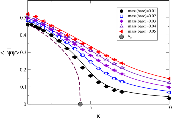
Figure 2: The corrected plot of the chiral condensate and the equation of state fits on a fixed volume $16^{3}$.

for comparison the new equations of state, together with the fitted data and the extrapolation to the chiral limit $m\to 0$, are plotted in Fig. 3. The following features are perhaps the most intriguing. The critical indices are compatible for both fits – however, the value of $\kappa_{c}$ is not only different from the value $\kappa_{c}=4.35(2)$ derived from fitting to the $16^{3}$ data alone [15], but is significantly different between the two forms of the finite scaling fit. This suggests not only that finite size effects play a significant role in the behaviour of this system, but that the effects of the anisotropy should be taken into consideration in future studies of the system. It is also worth noting that the value of the ${\chi^{2}}/{d.o.f.}$ is significantly better for the anisotropic scaling. Note also that for the weakly anisotropic fit, the sign of the coefficient of $L_{2}$, $D$ is different from those of $L_{1}$ and $L_{3}$, $C$ and $E$. This may reflect the expectation following (15) that $\xi_{2}\gg L$ over a much wider region of $\kappa$ than is the case for the other two directions. Contra the fitting results of [15], which were confined to a single lattice size, $\rho\approx 1.00$ with both equations; however, it is plausible that this is due to an insufficient spread of mass values in the data set.

Whether the actual value of the weakly anisotropic $\kappa_{c}$ is in fact 12.3(6) seems doubtful; we must note that the extrapolation is well outside the region of $\kappa$ for which we have any data. An interesting possibility is that it could also indicate that there is no phase transition and that the fit could be attempting to compensate for its absence by giving it a value in the unexplored region. If this behaviour were to persist for a more extensive data set, this hypothesis could be validated.

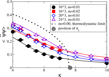
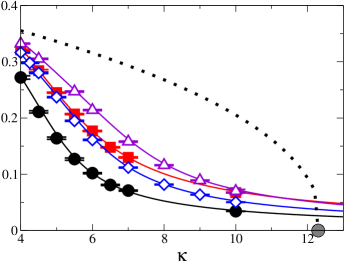
a)                                                                b)

Figure 3: Equation of state fits for (a) the isotropic case, and (b) the anisotropic case on various lattice sizes and in the thermodynamic, zero mass limit. $16^{3}$ results are taken from [15].

4 Scalar Sector

The scalar meson is the parity partner of the pseudoscalar pion bound state studied in [15]. In a phase with broken chiral symmetry the pion is a Goldstone boson, and hence is much lighter than the scalar. One signal for restoration of chiral symmetry is the recovery of degeneracy between scalar and pseudoscalar in the $m\to 0$ limit. The propagator of the scalar is defined in terms of the fermion fields as follows:

$$C_{\sigma\mu}(x_{\mu})=\sum_{\nu\not=\mu}\sum_{x_{\nu}}\langle\bar{\chi}\chi(0)\bar{\chi}\chi(x)\rangle.$$ (20)

Due to the nature of the flavour structure of staggered lattice fermions, propagation in this channel is prone to mixing with low mass bound states with different spin quantum numbers [24]. Where this contamination is significant, the propagator takes on a sawtooth shape, and we must thus fit a four parameter function, such as that in (22) below, so that we can distinguish propagation in the channel of interest.

In the following we distinguish between propagation in the Euclidean time direction $\tau$, yielding information on the excitation spectrum in the channel in question, eg. the bound-state mass, and propagation in the spatial directions $x$, $y$, where the corresponding quantity is the inverse screening length. Of course, in an isotropic system the two cases are equivalent in the infinite volume limit.

4.1 Temporal propagator

Least squares fitting of the function

$$C_{\sigma\,\mu}(x_{\mu})=A(e^{-m_{\sigma\,\mu}x_{\mu}}+e^{-m_{\sigma\,\mu}(L_{\mu}-x_{\mu})}),$$ (21)

(with $\mu$ chosen to be $\tau$) to data from $16^{3}$ lattices proved to be difficult within the chirally broken phase – the propagator data was exceedingly noisy, and care had to be taken in order to isolate the ground state signal from the excited states – but as the values moved into the chirally restored region the procedure became easier to perform. The results are listed in Table 2, and plotted in the graph 4, alongside the pion masses of [15] for each bare mass at $\kappa=10.00$.

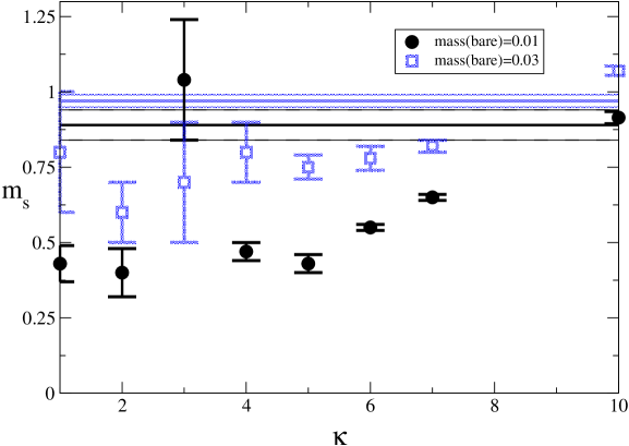
Figure 4: Scalar masses in the $\tau$ direction. Straight lines represent the pion masses at $\kappa=10.00$, taken from [15]. $m=0.05$ values are omitted due to the size of their error bars.

It can be seen from the figure that there are two regimes of scalar behaviour; below $\kappa_{c}$, where fitting is quite difficult, $m_{\sigma}$ is more or less constant as $\kappa$ increases (if we go by the $m=0.01$ data and ignore the outlier at $\kappa=3.00$) up to $\kappa\approx 5$ (ie. $\kappa\approx\kappa_{c}$ as estimated on $16^{3}$), whereupon we find that $m_{\sigma}$ begins to converge with $m_{\pi}$ as $\kappa$ increases into the chirally restored region. Figure 5 shows this in more detail for $m=0.01$.

We should point out that the jump in the value of $m_{\sigma\,\tau}$ at $\kappa=3.00$ and $m=0.01$ (and likely that of $m_{\sigma\,y}$ at $\kappa=4.00$, $m=0.05$, see below) is likely to be due to the frequent occurrence of abnormally small eigenvalues of the Dirac operator that overlapped with the meson source during our measurement of the propagator, similar to that seen in the Thirring model simulations of [25].

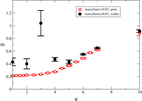
Figure 5: Scalar and pion masses (from [15]) in the $\tau$ direction for $m=0.01$.

The overall trend is consistent with the scalar becoming degenerate with the pion at large $\kappa$, consistent with manifest chiral symmetry. There is thus no evidence for persistence of chiral symmetry breaking at large $\kappa$ from the light meson spectrum.

$m$	$\kappa$	$m_{s}$	$\chi^{2}/d.o.f.$	fit window
0.01	1.00	0.43(6)	1.991	2-14
	2.00	0.40(8)	1.882	2-14
	3.00	1.04(2)	1.323	1-15
	4.00	0.47(3)	1.045	1-15
	5.00	0.43(3)	1.144	5-11
	6.00	0.55(1)	1.119	1-15
	7.00	0.65(1)	0.339	1-15
	10.00	0.91(2)	0.984	3-13
0.03	1.00	0.8(2)	1.177	2-14
	2.00	0.6(1)	1.089	2-14
	3.00	0.7(2)	0.923	2-14
	4.00	0.8(1)	0.397	2-14
	5.00	0.75(4)	1.351	2-14
	6.00	0.78(4)	0.983	3-13
	7.00	0.82(2)	0.505	1-15
	10.00	1.07(2)	1.273	1-15
0.05	1.00	1.0(2)	2.519	2-14
	2.00	1.2(7)	1.036	2-14
	3.00	0.6(1)	1.806	2-14
	4.00	1.0(2)	0.745	2-14
	5.00	1.4(1)	0.739	2-14
	6.00	0.95(5)	1.376	2-14
	7.00	1.05(5)	0.635	2-14
	10.00	1.16(2)	0.662	1-15

Table 2: Scalar masses $m_{sc\,\tau}$ in the $\tau$ direction on a $16^{3}$ lattice, for various masses.

4.2 Spatial propagators

$m$	$\kappa$	$m_{sx}$	$\chi^{2}/d.o.f$	fit window
0.01	1.00	0.32(4)	1.052	2-14
	2.00	1.0(2)	0.856	1-15
	3.00	2(1)	0.874	1-15
	4.00	1.04(8)	0.645	1-15
	5.00	1.28(3)	1.215	1-15
	6.00	1.53(2)	1.153	1-15
	7.00	1.83(2)	0.734	1-15
	10.00	2.62(2)	0.55	1-15
0.03	1.00	0.7(2)	1.643	2-14
	2.00	1.2(2)	1.495	1-15
	3.00	1.7(7)	1.021	1-15
	4.00	1.8(3)	0.577	1-15
	5.00	2.3(2)	1.09	1-15
	6.00	2.2(1)	1.596	1-15
	7.00	2.3(1)	0.984	2-14
	10.00	2.80(3)	0.853	1-15
0.05	1.00	0.7(1)	2.485	2-14
	2.00	1(1)	0.47	2-14
	3.00	2.2(4)	0.981	1-15
	4.00	3(3)	0.967	1-15
	5.00	2.5(4)	0.842	1-15
	6.00	2.6(2)	0.637	1-15
	7.00	2.8(2)	0.906	1-15
	10.00	3.20(7)	1.029	1-15

Table 3: Effective scalar mass $m_{s\;x}$ in the $x$ direction.

The spatial scalar masses were also obtained by least squares fitting to the propagator. For the $x$-direction (Table 3) and the $\kappa=1.00$ $y$-direction correlation functions, we used the fit function (21), and selected the fit window so as to exclude higher mass states. For $\kappa>1.00$, the $y$-direction correlation function exhibits a saw-tooth behaviour, motivating the following fit:

$$C_{\sigma\,y}=A(e^{-m_{\sigma\,y}y}+e^{-m_{\sigma\,y}(L_{y}-y)})+(-1)^{y}B(e^{-My}+e^{-M(L_{y}-y)}),$$ (22)

which proved acceptable across the full range of $\kappa$ if a fixed fitting window of spaceslices 1-15 was used. As with the temporal scalar propagators, those in the chirally symmetric phase were easier to fit than those in the chirally broken phase. It is also worth noting that in the symmetric phase the value of the correction mass $M$ was often consistent with zero for $m=0.01$ and $m=0.03$.

$m$	$\kappa$	$m_{\sigma y}$	$\chi^{2}/d.o.f$	fit window
0.01	1.00	0.41(6)	0.56	2-14
	2.00	0.25(5)	1.469	1-15
	3.00	0.2(1)	1.923	1-15
	4.00	0.13(2)	1.548	1-15
	5.00	0.09(2)	2.142	1-15
	6.00	0.1(2)	1.227	1-15
	7.00	0.1(5)	0.608	1-15
	10.00	00(11)	1.735	1-15
0.03	1.00	0.8(2)	0.721	2-14
	2.00	0.59(7)	1.732	1-15
	3.00	0.7(3)	1.076	1-15
	4.00	0.50(6)	7.661	1-15
	5.00	0.15(4)	1.015	1-15
	6.00	0.12(9)	1.351	1-15
	7.00	0.10(8)	0.798	1-15
	10.00	0.1(2)	1.55	1-15
.05	1.00	0.9(2)	0.676	2-14
	2.00	2.9(6)	8.468	1-15
	3.00	0.8(3)	4.308	1-15
	4.00	0.28(7)	1.315	1-15
	5.00	0.19(5)	2.097	1-15
	6.00	0.15(4)	1.636	1-15
	7.00	0.12(5)	1.818	1-15
	10.00	0.1(3)	1.87	1-15

Table 4: Effective scalar mass $m_{\sigma y}$ in the $y$ direction.

We have plotted $m_{\sigma\;x}$ against $\kappa$ in Figure 6, and $m_{\sigma\;y}$ against $\kappa$ in Figure 7. The trends previously observed for pions in [15] are repeated here: the value of $m_{\sigma\,x}$ increases with $\kappa$. In addition, as we have seen with $m_{\sigma\,\tau}$, it appears that there is convergence between the $m_{\sigma\,x}$ and the $m_{\pi\,x}$ values, most notably for $m=0.01$ (compare $m_{\sigma\,x}=.32(4)$ and $m_{\pi\,x}=.211(1)$ at $\kappa=1.00$ with $m_{\sigma\,x}=2.62(2)$ and $m_{\pi\,x}=2.58(2)$ at $\kappa=10.00$). Just as in Fig. 4, there is a change in behaviour around $\kappa\approx 5$, suggesting a change in behaviour as the scalar masses begin to converge on the pion masses within the chirally symmetric phase, once again consistent with the pion and scalar being parity partners.

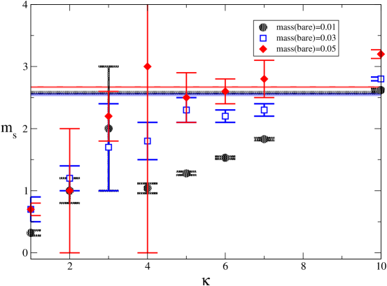
Figure 6: The scalar screening mass in the $x$-direction, $m_{s\;x}$, on a $16^{3}$ lattice. The straight lines represent $m_{\pi\,x}$ at a value of $\kappa=10.00$.

In the case of the $y$-direction masses, there is no pion data within the chirally symmetric phase with which to compare our results. The quality of the scalar data is also not that good, for the reasons mentioned above. It is less clear whether the change in the behaviour between phases is present here; it is likely to be quite small, and in any case the errors easily obscure it. Our only conclusion is, then, that the value of $m_{\sigma\;y}$ decreases as we increase $\kappa$; this is reinforced by the behaviour of the geometric mean of $m_{\sigma\;y}$ and $m_{\sigma\;x}$ above $\kappa\approx 5\approx\kappa_{c}$,

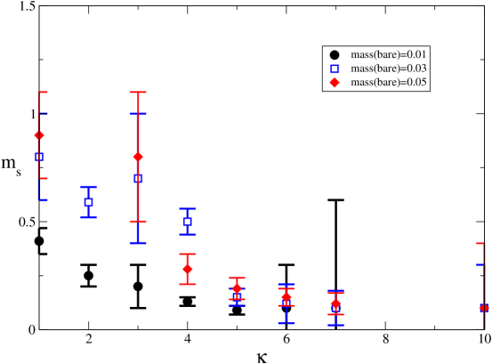
Figure 7: The scalar screening mass in the $y$-direction, $m_{s\;y}$, on a $16^{3}$ lattice. We omit the anomalous $m=0.05$, $\kappa=2.00$ value since its inclusion obscures the general trend of the data, and the $m=0.01$, $\kappa=10.00$ value due to the size of its error bars.

(Fig. 8); while there is a slight increase as we approach $\kappa_{c}$ (though the large error bars make it difficult to determine to what extent this is a genuine effect), above it, the geometric mean appears to remain fairly constant, which implies that $m_{\sigma\;y}$ is decreasing, as $m_{\sigma\;x}$ is increasing in this region.

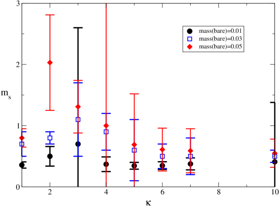
Figure 8: The geometric mean of the scalar screening masses, $\sqrt{m_{s\;y}m_{s\;x}}$, on a $16^{3}$ lattice.

4.3 Renormalised Anisotropy

Taking $\kappa_{R\,\sigma}$ to be the ratio of $m_{\sigma\,x}$ and $m_{\sigma\,y}$ (Figure 9), we find that it is relevant above $\kappa_{c}$ (more so, in fact, than for pions; Cf. Fig. 8 of [15]); however, in contrast to the pion case there appears to be a clear mass dependence below $\kappa_{c}$. It is difficult to tell whether this is a real effect or merely an artefact of the propagator fitting. On the assumption that the behaviour for $m=0.01$ is more or less linear, we fitted the data for $1.00\leq\kappa\leq 7.00$ to

$$R_{\sigma}=\frac{(\kappa_{R\,\sigma}-1)}{(\kappa-1)},$$ (23)

and acquired $R_{\sigma}=2.8(1)$, with $\chi^{2}/d.o.f.=1.77$. This appears slightly larger than $R_{\pi}\simeq 2.1$ [15], suggesting that the behaviour of scalar particles is affected by the anisotropy to a greater extent than that of the pions.

More data is needed before we can make definitive statements. In addition, it should be noted that we can’t rule out the existence of a change in behaviour around $\kappa_{c}$ for the values of $\kappa_{R\,\pi}$ – the pion data of [15] doesn’t extend far enough.

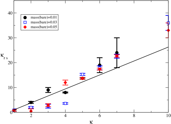
Figure 9: The renormalised $\kappa$ with respect to scalars, $\kappa_{R\,\sigma}$, on a $16^{3}$ lattice, together with a linear fit for $m=0.01$ (the dashed line is the quadratic fit, the filled line the linear). $\kappa=10.00$ has been omitted due to the size of the error bars.

Based on the parity partnership of pions and scalars, we propose the following hypothesis: that in the chirally restored phase, the magnitude of $\kappa_{R\,\sigma}$ will gradually approach that of $\kappa_{R\;\pi}$. The required data would best be generated on considerably larger lattices, with better statistics and perhaps with improved operators in order to avoid some of the issues with the data examined here.

5 Fermion Sector

In this section we report for the first time on studies of the fermion propagator $\langle\chi(x)\bar{\chi}(y)\rangle$. Large non-perturbative corrections to this Green function in the chiral limit $m\to 0$ have been proposed as an explanation of non-Fermi liquid behaviour in the non-superconducting region of the cuprate phase diagram [1]. An important challenge, both technical and conceptual, which must be faced is that the fermion propagator in QED is not a gauge invariant object, and can only by calculated, either analytically or numerically, if a gauge-fixing procedure is specified [26]. The dependence of the results on the choice of gauge is a thorny issue [27, 28, 16, 29]; here we will content ourselves with specifying Landau gauge, ie. $\partial_{\mu}A_{\mu}=0$ in continuum notation (implying that only transverse degrees of freedom are retained in the photon propagator), and performing a fully non-perturbative calculation on a $16^{3}$ lattice. In what follows we will first devote some considerable attention on the technicalities of fixing an unambiguous gauge for lattice gauge fields $U_{\mu}$, and then report our results for the fermion propagator. Our strategy in this exploratory study is to calculate the physical (ie. renormalised) fermion mass $m_{f}$ for fixed bare mass $m$ as a function of the anisotropy parameter $\kappa$. Apart from the fact that this is the simplest quantity to extract (by fitting to a decaying exponential), there is the theoretical motivation that $m_{f}$, given by the position of a pole in the complex $k$-plane, is gauge-invariant, at least to all orders in perturbation theory. As previously, we will distinguish between propagation in temporal and spatial directions.

5.1 Gauge Fixing

In order for the measurement of a gauge variant quantity such as the fermion propagator to be performed, we must impose a gauge condition which selects a unique set of gauge configurations from the infinite number of copies generated by local gauge transformations of the form (in this subsection we will denote the lattice site by a suffix)

$$\theta_{\mu x}\mapsto\theta^{\alpha}_{\mu x}=\theta_{\mu x}+\partial_{\mu}\alpha_{x},$$ (24)

where on a lattice finite difference operators are defined:

$$\partial_{\mu}f_{x}=f_{x+\hat{\mu}}-f_{x};\;\;\;\bar{\partial}_{\mu}f_{x}=f_{x}-f_{x-\hat{\mu}};$$ (25)

and $\alpha_{x}$ is any scalar function defined on the lattice sites.

For this study, we shall impose a latticised form of the Landau gauge condition

$$\sum_{\mu}\bar{\partial}_{\mu}\theta^{\alpha}_{\mu x}=0,$$ (26)

which is the extremum of

$$F^{\alpha}[\theta]=\sum_{x}\sum_{\mu=1}^{3}(\theta_{\mu x}^{\alpha})^{2},$$ (27)

corresponding to the following functional in terms of continuum gauge fields:

$$F[A]=\int d^{3}xA_{\mu}(x)A^{\mu}(x).$$ (28)

In order to proceed, modifications will have to be made to this minimal gauge condition (henceforth referred to as mLandau gauge). This is because it suffers from the so-called Gribov ambiguity [30].

5.1.1 The Gribov problem in QED₃

When gauge fixing is performed non-perturbatively, it may always not be possible to guarantee that there is a unique minimum of the functional $F[\theta]$. In numerical simulations, this can lead to a distortion of the results due to the underlying ambiguity [31]. The problem is normally associated with non-Abelian gauge fields in the continuum; however, it exists for Abelian fields on the lattice due to the toroidal boundary conditions [32], which give rise to zero modes which cannot be removed by local gauge transformations and is especially acute for compact (cQED₃) formulations of the gauge fields as it allows for the existence of topological defects (such as double Dirac strings in $2+1$ dimensions or double Dirac sheets in $3+1$ dimensions) whose creation or annihilation leaves the action unchanged [33].

Since we make use of a non-compact formulation of QED₃  (ncQED₃  ) in this study, it seems that the only problem we might have to deal with is the former. The modified iterative Landau gauge (miLandau gauge) [34, 35, 36] has often been used in order to deal with the problems due to the existence of zero-modes created by the boundary conditions of the lattice; however, it has not (as far as we are aware) been checked that there are any other sources of Gribov copies in this gauge. So, in what remains of this section, we shall describe miLandau gauge and present results that demonstrate that it does deal with the problem effectively, at least for the values of the parameters simulated in this paper.

5.1.2 The miLandau gauge for ncQED₃

Firstly, we note that on the lattice we cannot rotate $\theta^{\alpha}_{\mu}\mapsto\theta^{\alpha}_{\mu}+a_{\mu}$, where $a_{\mu}$ is an arbitrary constant vector field, if we wish to preserve the gauge invariance of the Polyakov and Wilson lines (defined to be products of the parallel transporters $U_{\mu\,x}$ along contours which are closed by periodic boundary conditions in the temporal and spatial directions, respectively). Instead, the form of the allowed gauge rotations is restricted to $a_{\mu}=\frac{n2\pi}{L_{\mu}}$, where $n$ is an arbitrary integer.

Using $\bar{\theta}_{\mu}=\frac{1}{V}\sum_{x}\theta_{\mu\,x}$ as the value of a constant background field (our zero-mode) we should expect the gauge degrees of freedom remaining after the mLandau gauge is fixed to vanish if we rotate

$$\theta^{\alpha}_{\mu}\mapsto\theta^{\alpha}_{\mu}+\frac{n2\pi}{L_{\mu}}$$ (29)

such that $-\frac{\pi}{L_{\mu}}<\bar{\theta}_{\mu}\leq\frac{\pi}{L_{\mu}}$.

• We fix mLandau gauge using a steepest descent algorithm [38]:

  • Given a gauge configuration {$\theta$}, for each site we calculate the value of $G_{x}=\sum_{\mu}\bar{\partial}_{\mu}\theta_{\mu x}$.

  • If $\frac{1}{V}\sum_{x}G_{x}<R$, where $R$ the floating point value $10^{-6}$, we terminate the algorithm here. Otherwise, we continue.

  • We rotate $\theta_{\mu x}\mapsto\theta_{\mu}(x)-\partial_{\mu}\chi_{x}$ on every link of every lattice site, where $\chi_{x}=\eta G_{x}$, and $\eta$ is a tunable parameter (here set to a value of $0.2$), used to optimise convergence.

  • We repeat until the halting criterion is fulfilled.

• Once mLandau gauge fixing is complete, we calculate $\bar{\theta}_{\mu}$ for $\mu=\hat{1}$.

• If $\bar{\theta}_{\mu}\leq-\frac{\pi}{L_{\mu}}$:

  • Add $\frac{2\pi}{L_{\mu}}$ to each $\theta_{\mu x}$ until $-\frac{\pi}{L_{\mu}}<\bar{\theta}_{\mu}\leq\frac{\pi}{L_{\mu}}$.

• If $\bar{\theta}_{\mu}>\frac{\pi}{L_{\mu}}$:

  • Subtract $\frac{2\pi}{L_{\mu}}$ to each $\theta_{\mu x}$ until $-\frac{\pi}{L_{\mu}}<\bar{\theta}_{\mu}\leq\frac{\pi}{L_{\mu}}$.

• Otherwise, leave each $\theta_{\mu x}$ unchanged.

• Repeat the above for the remaining directions $\mu=\hat{2},\,\hat{3}$.

5.1.3 A test of this prescription in ncQED₃

We wish to check that miLandau gauge removes Gribov copies from our measurements, by testing the effects of imposing miLandau gauge on randomly generated gauge copies of a set of gauge configurations [39, 40]. The results were generated for $\kappa=1.00$ and $\kappa=10.00$ on a $16^{3}$ lattice for $\beta=0.2$ and $m=0.03$, the extreme values of the range at which we wish to measure the propagator. 200 mother configurations were generated, and for each mother we created three 500 configuration ensembles corresponding to one of the following random gauge transformations:

• • • For all $x$ and $\mu$, $\theta_{\mu x}\mapsto\theta_{\mu x}-\partial_{\mu}\alpha_{x}$ where $\alpha_{x}$ is a random number between $-$9 and 9.

    • For all $x$ and $\mu$, $\theta_{\mu x}\mapsto\theta_{\mu x}+n_{\mu}\frac{2\pi}{L_{\mu}}$, where $n_{\mu}$ is a random integer – either 1, 0 or $-$1.

    • We perform both the transformation performed on Group A and that performed on Group B.

During the gauge fixing of each configuration, we monitored both the average value, $F_{av}$ of the gauge fixing functional (27) at each site and the value of the the function $L=\frac{1}{V}\sum_{x}G_{x}$, with $G_{x}$ defined in §5.1.2, for each iteration of the fixing. The behaviour of these parameters for a typical configuration is shown in Figure 10.

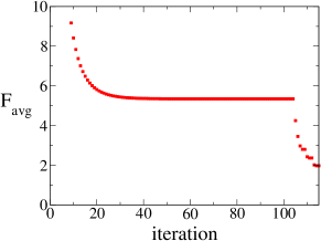
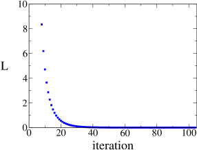
a)                                                       b)

Figure 10: Typical behaviour of $F_{av}$ (a) and $L$ (b) during gauge fixing. The plateau towards the middle of (a) corresponds to the area where (b) is converging on zero (that is to say, approaching mLandau gauge); the fall off beyond the hundred and fourth interaction is due to the imposition of full miLandau gauge. The first few points of both plots have been omitted so that this behaviour is visible.

We may also define a ‘variance’ $dF$ [37], which measures the difference in the minimised values of the gauge functional $F_{min}$ in a particular ensemble of a mother and associated daughter copies:

$$dF=\mbox{max}_{ij}[F_{min\>i}-F_{min\>j}].$$ (30)

with $i,j=1,\ldots,N$ where $N$ is the number of daughter configurations in the ensemble. If there are no Gribov copies present, this quantity should be zero (more realistically, in a numerical simulation we expect it to be of the order of the residual, $10^{-7}$), otherwise we expect a large value.

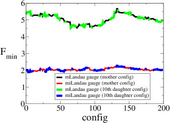
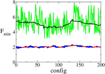
A                                                       B, C

Figure 11: Plots of $F_{min}$ at $\kappa=1.00$ for Groups A, B and C. $F_{min}$ for B and C are identical to within $10^{-7}$.

The results of our simulations at $\kappa=1.00$ and $\kappa=10.00$ with respect to Gribov copies were identical; we display figures for the former case, but our comments should be interpreted as generalising over both values of $\kappa$. Figures 11 and 12 plot $F_{min}$ and $dF$ for the ensembles generated using each procedure.

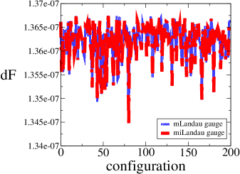
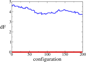
A                                                     B, C

Figure 12: Plots of the variance $dF$ at $\kappa=1.00$ for Groups A, B and C. $dF$ for B and C are identical to within $10^{-7}$.

• • • Here we find that while the value of $F_{min}$ is appreciably different in miLandau gauge from that in mLandau gauge (indicating that zero modes exist and have been gauge rotated away in the former), $dF$ is of the order of $10^{-7}$, suggesting that the random gauge transformations used here do not usually generate Gribov copies.

    • Unlike the above case, here we can see that there are in fact Gribov copies in the mLandau gauge: $dF$ is between 4 and 5 for $\kappa=1.00$ and 5 and 6 for $\kappa=10.00$. However, this is not the case for miLandau gauge. Here, as before, $dF$ in miLandau gauge is of the order of $10^{-7}$, and thus we can conclude that it rids us of the Gribov copies introduced by the random gauge transformation.

    • Here, the crucial observation is that (to within $10^{-7}$), the results for these random gauge transformations are identical to those of Group B. Indeed, it would be worrying were it otherwise; the effects of the two sets of transformations should be additive, so one would expect only Group B’s transformations to have any effect.

It is clear from the above that only shifts in the constant background field appear to contribute to gauge copies, and these are readily dealt with through the addition of further constraints to the minimal gauge fixing condition, via the choice of miLandau gauge. This stands in strong contrast to the case of cQED₃, where the compact Wilson gauge action allows for the existence of additional topological defects [33] which are also solutions of the equations of motion and therefore are Gribov copies.

This ‘desert landscape’ with respect to Gribov copies is not a disappointment – in fact, it is precisely the situation desired; one can be sure that the gauge has been fixed as in an unambiguous fashion.

5.2 The Fermion Propagator

In this section, we present measurements of the fermion propagator in the temporal and spatial directions:

$$C_{f\mu}(x_{\mu}) = \sum_{\nu\not=\mu}\sum_{x_{\nu}=A}\langle\chi(0)\bar{\chi}(x)\rangle,$$

$$A = \left\{\begin{array}[]{cc}2y_{\nu}&\mbox{Even numbered slice}\\ 2y_{\nu}+\hat{\mu}&\mbox{Odd numbered slice}\end{array}\right.$$ (33)

where the sum on $x$ only includes sites which are displaced from the origin by an even number of lattice spacings in each of the two transverse directions [24, 26]. We have also imposed noncompact miLandau gauge using the procedure outlined in §5.1.2. As mentioned previously, the calculation of $C_{f\mu}$ required the generation of around 30,000 trajectories of mean length 1.0 per $\kappa$-point in order to extract a signal from the considerable noise; for a dynamical fermion simulation this amounts to a large effort, requiring between one and three weeks per point to complete. Because of this difficulty, the error bars of our measurements remain sizable.

5.2.1 Temporal propagator

We extracted the fermion mass $m_{f\tau}$ in the temporal direction from the propagator data via the function

$$C_{f\,\tau}(\tau)=A(e^{-m_{f\,\tau}\tau}-(-1)^{\tau}e^{-m_{f\,\tau}(L_{\tau}-\tau)})$$ (34)

using correlated least-squares fitting; the results are recorded in Table 5 and Figure 14.

First we should first examine Figure 13, which shows examples of fermion propagators in the chirally restored phase $\kappa>0.5$. The following should be noted:

• The central area of each propagator is fairly flat, with large error bars (true of both phases). In this region the signal is overwhelmed by the noise and is consistent with zero. The size of the window containing data points exhibiting this behaviour decreased as the number of configurations in the sample was increased, suggesting that the cause is insufficient statistics. Because of this, it proved necessary to use fitting windows that are wider than the noisy region in order to extract a mass from the propagator. As in previous studies of elementary fermion propagation [24], no indication of contamination from excited states was seen within those windows.

• Figure 13 also illustrates an interesting feature of the fermion propagators for $\kappa>5$: the onset of a sawtooth-type behaviour visible in the logarithmic plots that, although relatively small, grows more pronounced with increasing $\kappa$. Since it is hard to distinguish it from noise, we performed fits of (34) to i) all of the timeslices and ii) to only the odd numbered timeslices for the propagators exhibiting this behaviour. Ideally, a four-parameter fit is preferred to ii), but these proved to be unstable.

The lines of best fit for both i) and ii) are included in Figure 13 for purposes of comparison, and the masses extracted are included in Table 5 and Figure 14.

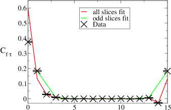
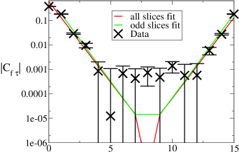
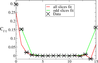
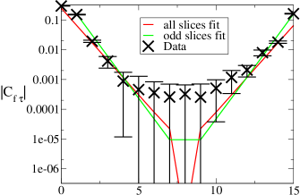
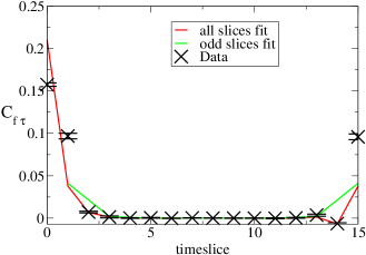
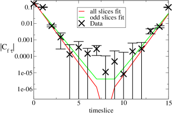
a)                                                         b)

Figure 13: Comparison of all timeslice and odd timeslice fits on (a) a linear scale, and (b) logarithmic scales for $\kappa$ of 6.00, 7.00 and 10.00 in descending order The errorbars represent unbinned, raw, statistical errors.

It is worth discussing the origin of the sawtooth behaviour. The chiral symmetry preserved by the lattice model (4,5) in the limit $m\to 0$ is the U(1) rotation

$$\chi(x)\mapsto\exp(i\beta\varepsilon(x))\chi(x);\;\;\;\bar{\chi}(x)\mapsto\exp(i\beta\varepsilon(x))\bar{\chi}(x);$$ (35)

where the phase $\varepsilon(x)\equiv(-1)^{x_{1}+x_{2}+x_{3}}$ distinguishes between even ($e$) and odd ($o$) sites. In the chiral limit the only non-vanishing entries of the fermion propagator matrix are $M^{-1}_{oe}$ and $M^{-1}_{eo}$; for small but non-zero $m$ it should still be the case in the chirally-symmetric phase that $|M^{-1}_{oe}|,\,|M^{-1}_{eo}|\gg|M^{-1}_{ee}|,\,|M^{-1}_{oo}|$. In the timeslice correlator $C_{f\mu}(x_{\mu})$ defined in (33) this implies that the signal should be much larger if $x_{\mu}$ is odd. Figure 13 shows that the sawtooth behaviour of the curve is not especially pronounced, and it is at present unclear to what extent the phenomenon is connected with the restoration of chiral symmetry.

	$\kappa$	$m$	$\chi^{2}/d.o.f.$	fit window
	1.00	1.00(2)	1.753	2-14
	3.00	1.17(2)	1.696	1-15
fit	4.00	1.33(7)	0.919	2-14
all timeslices	5.00	1.56(3)	0.827	1-15
	6.00	1.5(2)	1.211	2-14
	7.00	1.3(2)	1.031	2-14
	10.00	1.7(5)	1.015	2-14
fit only	6.00	1.58(9)	0.546	1-15
odd timeslices	7.00	1.6(1)	1.228	1-15
	10.00	1.8(2)	0.863	1-15

Table 5: Fermion masses $m_{f\,\tau}$ in the $\tau$ direction on a $16^{3}$ lattice, with $m=0.03$.

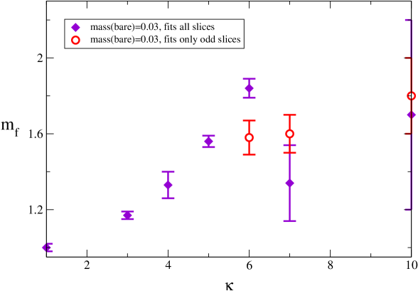
Figure 14: The renormalised fermion mass, $m_{f}$, measured in Landau gauge on a $16^{3}$ lattice for $m=0.03$.

Fig. 14 shows that for $\kappa\leq 5.00$, $m_{f\,\tau}$ increases with $\kappa$. The behaviour above $\kappa=5$ depends on the the type of fit – for fit ii) we see that the behaviour shows a non-zero mass in the region, which is more or less constant . Fit i) also shows the existence of a non-zero mass, but with more noise, possibly since it does not account for the sawtooth behaviour.

Regardless of the method chosen for the fitting of the propagators, there is a clearly a non-zero dynamically generated fermion mass in the chirally restored phase. This is unexpected – dynamical mass generation usually implies $\langle\bar{\chi}\chi\rangle\neq 0$, and chiral symmetry restoration usually implies massless fermions (Cf. Figs. 14 and 17 of Ref. [24], illustrating light fermion propagation on a $16^{3}$ lattice in the chirally-symmetric phase of the 3$d$ Thirring model). This seems to indicate that we are observing an unusual kind of chiral symmetry restoration; we shall return to this issue in due course.

5.2.2 Spatial propagators

We fit the spatial propagators to the following function:

$$C_{f\mu}(x_{\mu})=A(e^{-m_{f\,\mu}x_{\mu}}+(-1)^{x_{\mu}}e^{-m_{f\,\mu}(L_{\mu}-x_{\mu})}):$$ (36)

the change in sign compared to eqn.(34) being due to the use of periodic boundary conditions for the fermion fields in spatial directions, and anti-periodic boundary conditions, consistent with the imaginary time formalism used in (1), in the temporal direction.

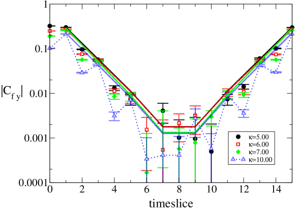
Figure 15: Plot of the fermion space-slice propagator, for $5.00\leq\kappa\leq 10.00$ on a $16^{3}$ lattice, along with the fitted curves. Note how the sawtooth behaviour becomes more prominent as $\kappa$ increases, except on timeslices between 6 and 10, where noise dominates. The errors here are unbinned.

Figure 15 shows the absolute values of propagators in the $y$-direction for $\kappa\geq 5.0$. The propagators exhibit a more pronounced form of the sawtooth behaviour than $C_{f\;\tau}$ ($C_{f\;x}$ do not exhibit this behaviour at all). Unlike in the case of the pions in [15], this is not due to the fermion becoming light, as one can surmise from the slope of the curve.

$\kappa$	$m$	$\chi^{2}/d.o.f.$	fit window
1.00	0.97(1)	2.540	1-15
3.00	1.6(2)	1.839	2-14
4.00	2.1(1)	1.233	1-15
5.00	2.7(2)	0.579	1-15
6.00	2.6(2)	1.097	1-15
7.00	3.6(7)	0.800	1-15
10.00	5(2)	0.793	1-15

Table 6: Fermion masses $m_{f\,x}$ in the $x$ direction on a $16^{3}$ lattice, with $m=0.03$.

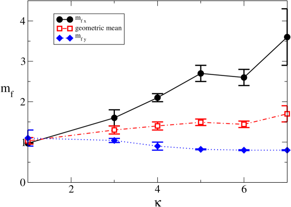
Figure 16: Fermion screening masses $m_{f\,x}$, $m_{f\,y}$, and the geometric mean $\sqrt{m_{f\,x}m_{f\,y}}$, versus $\kappa$, on a $16^{3}$ lattice. Lines do not correspond to fits.

As for the sawtoothed propagators in the $\tau$-direction, we performed fits only to odd $y$, as four-parameter fits proved unstable. The resulting screening masses are shown in tables 6 and 7.

	$\kappa$	$m$	$\chi^{2}/d.o.f.$	fit window
fit	1.00	1.1(2)	0.887	4-12
all timeslices	3.00	1.04(5)	0.951	3-13
	4.00	0.9(1)	0.907	4-12
	5.00	0.82(1)	2.475	1-15
fit only	6.00	0.80(1)	1.794	1-15
odd timeslices	7.00	0.80(1)	0.689	1-15
	10.00	0.80(1)	0.405	1-15

Table 7: Fermion masses $m_{f\,y}$ in the $y$ direction on a $16^{3}$ lattice, with $m=0.03$.

We can see that the fermions follow the same general trend as $\kappa$ increases as the pions in [15] – those in the $x$-direction grow heavier, and those in the $y$-direction grow lighter; anomalies in the data (e.g. at $\kappa=6.00$) are likely to be due to noise.

The geometrical mean $\sqrt{m_{f\;x}m_{f\;y}}$ increases from 1 to $\sim 1.75(20)$ as we move into regions of large anisotropy, which suggests that some small dynamical effect may come into play over and above that of the anisotropies themselves. This could correspond to a renormalisation of the parameter $\delta$ in Lee and Herbut’s model to a value other than unity, as $\sqrt{(\delta\lambda a)(\delta\lambda^{-1}a)}=\delta a$ [8].

5.2.3 Renormalised anisotropy:

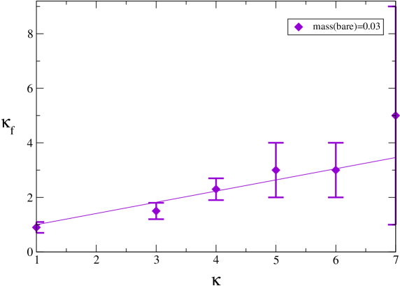
Figure 17: The renormalised $\kappa$, $\kappa_{r\,f}$, together with a fitted curve, on a $16^{3}$ lattice.

The renormalised fermion anisotropy $\kappa_{R\,f}=m_{f\,x}/m_{f\,y}$ is displayed in Figure 17. It is a measurement of the relevance of $\kappa>1$ relative to the particle in question. We find that the anisotropy parameter for fermions is irrelevant in the renormalisation group sense; that is

$$R_{f}=\frac{(\kappa_{R\,f}-1)}{(\kappa-1)}<1.$$ (37)

Indeed, if we fit the above function to the data for $1\leq\kappa\leq 7.00$, we find $R_{f}=.41(4)$, with a $\chi^{2}/d.o.f.$ of 1.67. This is striking, as the anisotropy is quite clearly relevant in the cases of pions [15], and scalars as shown in §4.3. The implication is that as $\kappa$ increases, the fermion – anti-fermion bound states become increasingly $1+1$-dimensional, only able to propagate in the $y-\tau$ plane (in the original condensed matter-inspired model (LABEL:eq:finalbit) $f\bar{f}$ excitations associated with the other “flavour”, ie. node pair, would be confined to the $x-\tau$ plane). The only excitations able to explore the whole $2+1$-dimensional space are the elementary fermions. This point will be further discussed below.

6 Discussion

Here we summarise the main results of our study, and speculate as to the behaviour of QED₃ as the anisotropy $\kappa$ is increased.

We applied a finite volume scaling analysis to data from $16^{3}$, $20^{3}$ and $24^{3}$ systems in an attempt to determine the order of the phase transition. There is no evidence for a diverging susceptibility as the volume increases, and remarkably the value $\kappa_{c}$ marking the apparent transition appears to be very sensitive to system size; our fits assuming an isotropic model of finite volume corrections yield $\kappa_{c}=7.66(5)$, which once the possibility of anisotropic corrections is admitted drifts out to $\kappa_{c}=12.3(6)$. Since the latter value lies outside our range of simulated parameters, it casts doubt on our original claim [15] that a true chiral symmetry restoring transition is taking place. Rather, an interpretation of the transition in terms of a crossover from strong to weak coupling regimes seems admissible – very similar to the transition observed in simulations of isotropic QED₃ [5, 17]. As in those studies, it appears to be a very difficult task to determine computationally whether chiral symmetry is actually broken in the weak coupling regime, reflecting the fact that QED₃ may be a model with an abnormally large separation between the scale of dynamical symmetry breaking $\Sigma$ and the natural mass scale $g^{2}$. It should be stressed, however, that the studies of the pion and scalar spectra in Sec. 4 are consistent with a chirally-restored vacuum at large $\kappa$.

What does seem clear is that any successful model of the finite volume scaling must take anisotropy into account – here our analysis assumed weak anisotropy, but models with differing critical exponents in different directions cannot be excluded. Unfortunately, the cure for these many uncertainties is to accumulate data from many more values of $L$ and $m$, which is beyond our current resources.

However, it is intriguing to note that from [15, 6], we can estimate that at $T=0$ we enter the dSC phase (and QED₃  ceases to be a valid effective field theory of the cuprates) somewhere in the region $6\raisebox{-2.15277pt}{$\ \stackrel{{\scriptstyle\textstyle<}}{{\textstyle\sim}}\ $}\kappa\raisebox{-2.15277pt}{$\ \stackrel{{\scriptstyle\textstyle<}}{{\textstyle\sim}}\ $}8$. Even taking the isotropic estimate $\kappa_{c}=7.66(5)$ as the correct one, therefore, it is uncertain whether the intermediate pseudogap phase between SDW and dSC can actually exist. This raises a matter of some importance to future research: if $\kappa$ affects the behaviour of the system, does it do so enough to make a difference in the condensed matter systems for which anisotropic QED₃  is intended as an effective theory?

Our studies of the propagation of $f\bar{f}$ bound states in the scalar channel showed evidence for degeneracy between scalar and pseudoscalar as $\kappa$ increases, although the propagator data are markedly noisier in the scalar case. This is consistent with chiral symmetry restoration, but bearing in mind the cautious note of the preceding paragraphs, we should note that a very soft symmetry breaking cannot be excluded. Another important result is that the renormalised anisotropy $\kappa_{R\sigma}\raisebox{-2.15277pt}{$\ \stackrel{{\scriptstyle\textstyle>}}{{\textstyle\sim}}\ $}\kappa_{R\pi}$, implying that anisotropy is a relevant perturbation for both sets of particles. More graphically, this means that for large $\kappa$ $f\bar{f}$ bound states are effectively constrained to propagate in just the $y$-direction, and their dynamics are essentially 1+1 dimensional.

The most significant result has emerged in the fermion sector, where we have found evidence that dynamical mass generation persists even once the apparent restoration of chiral symmetry has set in. Note that this result explains a rather surprising result reported in [15]; namely, the average plaquette action ${\beta\over 2}\langle\Theta_{\mu\nu}^{2}\rangle$ increases with $\kappa$, implying that screening due to virtual $f\bar{f}$ pairs in the quantum vacuum actually decreases with $\kappa$, in contradiction to what would be expected if light fermion degrees of freedom were important in the high-$\kappa$ regime. The sawtooth structure that develops as $\kappa$ increases may also be a sign of chiral symmetry restoration, although a study with $m$ varying, beyond our current resources, would be needed to confirm this hypothesis.

The fact that a non-zero dynamically generated fermion mass accompanies the chirally restored phase suggests that the symmetric phase is of an unusual kind. Witten [41] has examined a similar situation in the Gross-Neveu model in $1+1$ dimensions; $\langle\bar{\chi}\chi\rangle=0$ and a dynamically generated mass may coexist if the following are the case:

• The physical fermion is a branch-cut, not a pole, in momentum space, and lacks the same quantum numbers as the bare, massless fermion field $\psi$ (the former has zero chirality – i.e. is chirally neutral – whereas the bare fermion has a non-zero chirality). It follows that chiral symmetry tells us nothing about the value of the dynamically generated fermion mass – the system behaves in a chirally symmetric fashion in most respects apart from the existence of this mass.

• There exists a massless (pseudo)scalar boson, which interacts strongly with the fermion and carries the chiral current. Interactions between it and the $\psi$ field (which is distinct from the observed physical fermion) are chirality changing. The interaction between $\psi$ and the boson modifies the chirally asymmetric portion of the fermion propagator, causing it to vanish.

It is important to note that the scalar field in this example is not a Goldstone boson, which must be weakly-interacting. In the $1+1$ dimensional Gross-Neveu model the formation of Goldstone bosons is prohibited by the Coleman-Mermin-Wagner theorem [42, 43], which states the impossibility of spontaneously breaking a continuous global symmetry in $1+1$ dimensions. A similar phenomenon has been observed in simulations of the 2+1$d$ Gross-Neveu model at non-zero $T$ [44]. While perhaps it not clear how to define the effective dimensionality of an anisotropic theory, we take from this analogy the notion that infra-red fluctuations remain important in the chirally symmetric phase; in other words the interaction between fermion and scalar degrees of freedom is strong.

In support of this hypothesis applying in the current situation, we point out that the mass ratios $m_{f}:m_{\pi}:m_{\sigma}$ vary from $1:0.2:0.4$ at $\kappa=1$, consistent with broken chiral symmetry, to $1.8:0.9:0.9$ at $\kappa=10$, consistent with restored chiral symmetry, but in which the scalar bound states are still tightly bound and light compared with the fermion mass scale. This should be contrasted with the “orthodox” chiral symmetry restored scenario $m_{f}:m_{\pi}:m_{\sigma}\approx 0.5:1:1$ observed in the 3$d$ Thirring model and portrayed in Fig. 17 of [24].

It should be noted that the situation in which dynamical mass generation without symmetry breaking is observed is sometimes referred to as pseudogap behaviour. We must caution against confusing this with the pseudogap phase of the cuprate which we are modelling; while they share some behaviour in common (in both cases, we observe the phase disordering of an order parameter), they refer to different phenomena – the former referring to a phase of the putative effective theory, and the latter to that of the behaviour of the full description of the superconductor from which it is derived.

Another important observation in the fermion sector is that $\kappa_{Rf}<\kappa$ implying anisotropy is an irrelevant perturbation, i.e. fermions remain 2+1$d$ particles as $\kappa$ increases, although scalar-mediated interactions among the fermions must be anisotropic. It will be a theoretical challenge to formulate an effective description incorporating these features.

In many ways our study has raised more questions than it has answered; its main results have not been predicted by analytic treatments of the system performed so far. This may raise questions regarding the conception of the pseudogap in those models of HT_c superconductivity – such as that of [1] – which require the presence of massless fermions in the chirally symmetric phase, since it appears that the expected link between a non-vanishing chiral condensate and a dynamically generated fermion mass is broken. However, it is too early to make definitive statements; the fermion propagator should be measured in a number of gauges, so that we can be certain as to how much (if any) of the observed behaviour is an artefact of Landau gauge. Ultimately, more data on how the dynamically generated fermion mass behaves as the chiral, thermodynamic and continuum limits are approached will be needed. Anisotropic QED₃ appears to be every bit as computationally demanding and as fascinating as its isotropic counterpart.

References

- [1] M. Franz, Z. Tesanovic, and O. Vafek, Phys. Rev. B66, 054535 (2002), cond-mat/0203333.
- [2] I. F. Herbut, Phys. Rev. B66, 094504 (2002), cond-mat/0202491.
- [3] A. Kovner, B. Rosenstein, and D. Eliezer, Nucl. Phys. B350, 325 (1991).
- [4] O. I. Motrunich and A. Vishwanath, cond-mat/0311222.
- [5] S. J. Hands, J. B. Kogut, and C. G. Strouthos, Nucl. Phys. B645, 321 (2002), hep-lat/0208030.
- [6] M. Sutherland et al., cond-mat/0301105.
- [7] M. R. Presland, J. L. Tallon, R. Buckley, R. Liu, and N. Flower, Physica C176, 95 (1991).
- [8] D. J. Lee and I. F. Herbut, Phys. Rev. B66, 094512 (2002), cond-mat/0201088.
- [9] O. Vafek, Z. Tesanovic, and M. Franz, Phys. Rev. Lett. 89, 157003 (2002), cond-mat/0203047.
- [10] G. W. Semenoff, Phys. Rev. Lett. 53, 2449 (1984).
- [11] V. P. Gusynin and S. G. Sharapov, Phys. Rev. Lett. 95, 146801 (2005), cond-mat/0506575.
- [12] V. P. Gusynin and S. G. Sharapov, Phys. Rev. B71, 125124 (2005), cond-mat/0411381.
- [13] N. M. R. Peres, F. Guinea, and A. H. C. Neto, Phys. Rev. B73, 125411 (2006).
- [14] K. Novoselov et al., Nature 483, 197 (2005), cond-mat/0509330.
- [15] S. Hands and I. O. Thomas, Phys. Rev. B72, 054526 (2005), hep-lat/0412009.
- [16] M. Franz, Z. Tesanovic, and O. Vafek, cond-mat/0204536.
- [17] S. J. Hands, J. B. Kogut, L. Scorzato, and C. G. Strouthos, Phys. Rev. B70, 104501 (2004), hep-lat/0404013.
- [18] T. Appelquist and L. C. R. Wijewardhana, (2004), hep-ph/0403250.
- [19] X. S. Chen and V. Dohm, cond-mat/0408511.
- [20] V. Privman and M. E. Fisher, Phys. Rev. B30, 322 (1984).
- [21] J. O. Indekeu, M. P. Nightingale, and W. V. Wang, Phys. Rev. B34, 330 (1986).
- [22] A. Hucht, J. Phys. A35, 481L (2002).
- [23] S. Caracciolo, A. Gambassi, M. Gubinelli, and A. Pelissettio, Eur. Phys. J. B34, 205 (2003).
- [24] UKQCD, L. Del Debbio, S. J. Hands, and J. C. Mehegan, Nucl. Phys. B502, 269 (1997), hep-lat/9701016.
- [25] L. Del Debbio and S. J. Hands, Nucl. Phys. B552, 339 (1999), hep-lat/9902014.
- [26] M. Gockeler, R. Horsley, P. Rakow, G. Schierholz, and R. Sommer, Nucl. Phys. B371, 713 (1992).
- [27] D. V. Khveshchenko, Phys. Rev. B65, 235111 (2002), cond-mat/0112202.
- [28] D. V. Khveshchenko, Nucl. Phys. B642, 515 (2002).
- [29] D. V. Khveshchenko, cond-mat/0205106.
- [30] V. N. Gribov, Nucl. Phys. B139, 1 (1978).
- [31] V. K. Mitrjushkin, Phys. Lett. B390, 293 (1997), hep-lat/9606014.
- [32] T. P. Killingback, Phys. Lett. B138, 87 (1984).
- [33] V. K. Mitrjushkin, Phys. Lett. B389, 713 (1996), hep-lat/9607069.
- [34] M. Gockeler et al., Phys. Lett. B251, 567 (1990).
- [35] S. Durr and P. de Forcrand, Phys. Rev. D66, 094504 (2002), hep-lat/0206022.
- [36] A. Nakamura and R. Sinclair, Phys. Lett. B243, 396 (1990).
- [37] I. L. Bogolubsky, V. K. Mitrjushkin, M. Muller-Preussker, and P. Peter, Phys. Lett. B458, 102 (1999), hep-lat/9904001.
- [38] C. T. H. Davies et al., Phys. Rev. D37, 1581 (1988).
- [39] L. Giusti, M. L. Paciello, C. Parrinello, S. Petrarca, and B. Taglienti, Int. J. Mod. Phys. A16, 3487 (2001), hep-lat/0104012.
- [40] E. Marinari, C. Parrinello, and R. Ricci, Nucl. Phys. B362, 487 (1991).
- [41] E. Witten, Nucl. Phys. B145, 110 (1978).
- [42] N. D. Mermin and H. Wagner, Phys. Rev. Lett. 17, 1133 (1966).
- [43] S. R. Coleman, Commun. Math. Phys. 31, 259 (1973).
- [44] S. J. Hands, J. B. Kogut, and C. G. Strouthos, Phys. Lett. B515, 407 (2001), hep-lat/0107004.