Lattice simulations of real-time quantum fields

We investigate lattice simulations of scalar and nonabelian gauge fields in Minkowski space-time. For $SU(2)$ gauge-theory expectation values of link variables in 3+1 dimensions are constructed by a stochastic process in an additional (5th) “Langevin-time”. A sufficiently small Langevin step size and the use of a tilted real-time contour leads to converging results in general. All fixed point solutions are shown to fulfil the infinite hierarchy of Dyson-Schwinger identities, however, they are not unique without further constraints. For the nonabelian gauge theory the thermal equilibrium fixed point is only approached at intermediate Langevin-times. It becomes more stable if the complex time path is deformed towards Euclidean space-time. We analyze this behavior further using the real-time evolution of a quantum anharmonic oscillator, which is alternatively solved by diagonalizing its Hamiltonian. Without further optimization stochastic quantization can give accurate descriptions if the real-time extend of the lattice is small on the scale of the inverse temperature.

1 Introduction

Lattice gauge theory provides important insight into strongly interacting theories such as quantum chromodynamics (QCD). Typically, calculations are based on a Euclidean formulation, where the time variable is analytically continued to imaginary values. By this the quantum theory is mapped onto a statistical mechanics problem, which can be simulated by importance sampling techniques. Recovering real-time properties from the Euclidean formulation is a formidable problem that is still in its infancies. Direct simulations in Minkowski space-time would be a breakthrough in our efforts to resolve pressing questions, such as early thermalization or the origin of seemingly perfect fluidity in a QCD plasma at RHIC [2]. For real times standard importance sampling is not possible because of a non-positive definite probability measure. Efforts to circumvent this problem include mimicking the real-time dynamics by computer-time evolution in Euclidean lattice simulations [3, 4]. A problem in this case is to calibrate the computer time independently of the algorithm. Another procedure amounts to separate a positive factor from the Boltzmann factor to be used for importance sampling, and re-weight the configurations with the remaining (complex) part. These so-called “reweighting methods” suffer from the problem of large cancellations of contributions, induced by the oscillating signs in the weight (“sign problem”) and from the difficulty of ensuring a sufficient overlap between the simulated and the target ensemble (“overlap problem”).

Direct simulations in Minkowski space-time, however, may be obtained using stochastic quantization techniques, which are not based on a probability interpretation [5, 6]. In Ref. [7] this has been recently used to explore nonequilibrium dynamics of an interacting scalar quantum field theory.

In real-time stochastic quantization the quantum ensemble is constructed by a stochastic process in an additional “Langevin-time” using the reformulation for the Minkowskian path integral [8, 9, 10]: The quantum fields are defined on a $d$-dimensional physical space-time lattice, and the updating employs a Langevin equation with a complex driving force in an additional, unphysical “time” direction. This procedure does not involve reweighting, nor redefinition of the Minkowski dynamics in terms of an associated Euclidean one. Though more or less formal proofs of equivalence of the stochastic approach and the path integral formulation have been given for Minkowski space-time, not much is known about the general convergence properties and its reliability beyond free-field theory or simple toy models [9, 10]. More advanced applications concern simulations in Euclidean space-time with non-real actions [11, 12]. Besides successful applications, major reported problems in this case concern unstable Langevin dynamics and incidences of convergence to ”unphysical” results [13, 11, 12].

In this paper we discuss real-time stochastic quantization for scalar field theory and $SU(N)$ pure gauge theory relevant for QCD. Similar to what has been observed in Ref. [7] for scalar fields, also for the gauge theory we find that previously reported unstable dynamics represents no problem in practice. A combination of sufficiently small Langevin step size and the use of a ”tilted” real-time contour leads to converging results in general. Our procedure respects gauge invariance and appears to be well under control. This is exemplified for $SU(2)$ gauge theory in $3+1$ dimensions. For the scalar theory we consider, in particular, a zero-spatial dimension example, namely a quantum anharmonic oscillator. The latter is solved in addition by alternative methods using Hamiltonian diagonalization for comparison. We find that stochastic quantization can accurately describe the time evolution for lattices with sufficiently small real-time extent. This concerns nonequilibrium and equilibrium simulations at weak as well as strong couplings. However, when the real-time extent of the lattice is enlarged the stochastic updating does not converge to the correct solution. In particular, for the nonabelian gauge theory the thermal equilibrium solution is only approached at intermediate Langevin-times. Its life-time in the course of the Langevin evolution becomes longer if the complex time path is deformed towards Euclidean space-time.

Since there appears more than one fixed point to which the Langevin flow can converge, the solutions obtained by real-time stochastic quantization are not unique in general. Similar observations have been made before for Euclidean theories with complex actions [13]. Euclidean theories with real actions can be shown to have a unique solution based on positivity arguments [5]. A similar argument fails for real-time stochastic quantization. In general, here the correct fixed point cannot be chosen a priori without implementing further constraints. We prove that all possible fixed point solutions fulfil the same infinite set of (symmetrized) Dyson-Schwinger identities of the quantum field theory. However, solutions of Dyson-Schwinger equations without specifying further constraints are not unique in general. We discuss how tests for differentiating them can typically be devised and applied.

The paper is organized as follows. Sec. 2 reviews stochastic quantization in Euclidean space-time, which fixes the notation for the derivation of the real-time dynamics in Sec. 3. Particular emphasis is put on the developments for gauge theories, since previous suggestions for Langevin dynamics in the additional ”time” dimension violate Dyson-Schwinger identities of the original quantum theory. In Sec. 4 we prove Dyson-Schwinger equations to follow from real-time stochastic quantization. Simulation results and precision tests are discussed in Secs. 5 and 6. We end with conclusions in Sec. 7.

2 Euclidean stochastic quantization

The stochastic quantization algorithm calculates ensemble averages in an extended space of variables, where the lattice action $S$ of the $d$-dimensional quantum theory plays the role of a potential energy in a classical Hamiltonian $H$ of a ($d+1$)-dimensional, embedding theory. The ensemble averages of the original quantum theory are computed from classical evolution in the additional ”time” dimension.

2.1 Euclidean scalar theory

We first consider classical dynamics for scalar fields in $d$-dimensional Euclidean space-time with Hamiltonian (see e.g. [14])

$$H=\int\!{\rm d}^{d}x\left(\frac{1}{2}\pi^{2}(x;t_{5})+{\mathcal{L}_{\rm E}}(\varphi(x;t_{5}),\partial_{x}\varphi(x;t_{5}))\right)\,.$$ (1)

Here the field $\varphi$ and momentum $\pi$ depend on the $d$-dimensional Euclidean space-time variable $x_{\mu}$ ($\mu=0,\ldots 3$) and on an additional “time” variable $t_{5}$. The function ${\mathcal{L}_{\rm E}}$ depends on the field and its derivatives with respect to $x_{\mu}$. It is taken to correspond to the Lagrange density of the physical four-dimensional Euclidean field theory with mass $m$ and quartic self-interaction $\lambda$ where

$${\mathcal{L}_{\rm E}}=\frac{1}{2}\left\{\left(\partial_{x}\varphi(x;t_{5})\right)^{2}+m^{2}\varphi^{2}(x;t_{5})\right\}+\frac{\lambda}{4!}\varphi^{4}(x;t_{5})\,.$$ (2)

Since ${\mathcal{L}}$ contains no field derivatives with respect to $t_{5}$ the variable enters only as an additional field label in Eq. (2).

Expectation values of observables $F(\varphi)$ are given by the functional integral

$$\langle F(\varphi)\rangle=Z^{-1}\int{\cal D}\pi{\cal D}\varphi\,F(\varphi)\,e^{-H[\pi,\varphi]}$$ (3)

with the normalization

$$Z=\int{\cal D}\pi{\cal D}\varphi\,e^{-H[\pi,\varphi]}\,.$$ (4)

The Gaussian integrals over the momentum fields can be trivially performed and the overall constants cancel out in the computation of field expectation values. Here the introduction of the canonical field momenta is used to compute expectation values of quantum fields from classical Hamiltonian dynamics. This amounts to replacing the canonical ensemble averages (3) by micro-canonical ones. The latter can be obtained from solving Hamilton equations.

The basis for the numerical simulations are the discretized classical equations for the Hamiltonian (1). The classical dynamics of the field $\varphi$ and its conjugate momentum $\pi$ in $t_{5}$-time is described by Hamilton equations of motion

$$\frac{\partial\varphi(x;t_{5})}{\partial t_{5}} = \frac{\delta H}{\delta\pi(x;t_{5})}\,\,=\,\,\pi(x;t_{5})\,,$$ (5)

$$\frac{\partial\pi(x;t_{5})}{\partial t_{5}} = -\frac{\delta H}{\delta\varphi(x;t_{5})}\,\,=\,\,-\frac{\delta S_{\rm E}[\varphi]}{\delta\varphi(x;t_{5})}\,,$$ (6)

where the functional differentiation with respect to $\varphi$ is for fixed $t_{5}$. The Euclidean action is

$$S_{\rm E}[\varphi]\,\equiv\,\int{\rm d}^{d}x\,{\mathcal{L}_{\rm E}}(\varphi(x),\partial_{x}\varphi(x))\,.$$ (7)

In order to discretize Eqs. (5) and (6) in $t_{5}$, we denote the difference in subsequent $t_{5}$-time steps by $\Delta t_{5}\equiv(t_{5})_{n+1}-(t_{5})_{n}$. Correspondingly, we will write $\left\{\varphi((t_{5})_{n+1}),\pi((t_{5})_{n+1})\right\}\to\left\{\varphi^{\prime},\pi^{\prime}\right\}$ and $\left\{\varphi((t_{5})_{n}),\pi((t_{5})_{n})\right\}\to\left\{\varphi,\pi\right\}$. A suitable second-order discretization of (5) then reads

$$\varphi^{\prime}(x) = \varphi(x)+\frac{\partial\varphi(x)}{\partial t_{5}}\,\Delta t_{5}+\frac{1}{2}\frac{\partial^{2}\varphi(x)}{\partial t_{5}^{2}}\,\Delta t_{5}^{2}$$ (8)

$$= \varphi(x)+\pi(x)\,\Delta t_{5}-\frac{1}{2}\frac{\delta S_{E}[\varphi]}{\delta\varphi(x)}\,\Delta t_{5}^{2}\,.$$

Correspondingly, expanding $\pi^{\prime}-\pi$ to order $\Delta t_{5}$ and using Eq. (6) the field momenta are (leapfrog) evolved with

$$\pi^{\prime}(x)=\pi(x)-\frac{1}{2}\left(\frac{\delta S_{\rm E}[\varphi]}{\delta\varphi(x)}+\frac{\delta S_{\rm E}[\varphi^{\prime}]}{\delta\varphi^{\prime}(x)}\right)\,\Delta t_{5}\,,$$ (9)

which yields reversible and area preserving discretized dynamics [14].

The conjugate momenta in the classical Hamiltonian (1) have a Gaussian distribution, which is independent of the values of the field variables. If instead of stepping along a single classical trajectory the momenta after every single step are randomly refreshed, one recovers classical Langevin dynamics in $t_{5}$-time. It amounts to making the substitutions

$$\sqrt{2}\,\pi(x)\,\to\,\eta(x)\,,\qquad\frac{1}{2}\Delta t_{5}^{2}\,\to\,\epsilon\,,$$ (10)

with Gaussian noise

$$\langle\eta(x)\rangle_{\eta}=0\,,\qquad\langle\eta(x)\,\eta(x^{\prime})\rangle_{\eta}=2\,\delta(x-x^{\prime})\,,$$ (11)

where the average of an observable $A(\varphi;\eta)$ over the noise is given by

$$\langle A(\varphi;\eta)\rangle_{\eta}\equiv\frac{\int[{\rm d}\eta]\,A(\varphi;\eta)\exp\left\{-\frac{1}{4}\int\!{\rm d}^{4}x\,\eta^{2}(x)\right\}}{\int[{\rm d}\eta]\,\exp\left\{-\frac{1}{4}\int\!{\rm d}^{4}x\,\eta^{2}(x)\right\}}\,\,.$$ (12)

The discretized Langevin equation then reads

$$\varphi^{\prime}(x)=\varphi(x)-\epsilon\,\frac{\delta S_{\rm E}[\varphi]}{\delta\varphi(x)}+\sqrt{\epsilon}\,\eta(x)\,.$$ (13)

The sum over the Langevin steps, $\vartheta\equiv\sum\epsilon$, is called ”Langevin-time”, which replaces $t_{5}$ of the classical dynamics.

This simplified description of the classical dynamics forms the basis of stochastic quantization [5]. The stochastic process (13) is associated to a distribution $P_{\rm E}(t_{5})$ for the field $\varphi(x)$. Writing $P_{\rm E}((t_{5})_{n+1})\to P_{\rm E}^{\prime}$ and $P_{\rm E}((t_{5})_{n})\to P_{\rm E}$ its evolution can be obtained from

$$P^{\prime}_{\rm E}[\varphi^{\prime}]=\Bigg{\langle}\int[{\rm d}\varphi]P_{\rm E}[\varphi]\prod_{x}\delta\left(\varphi^{\prime}(x)-\varphi(x)+\epsilon\frac{\delta S_{\rm E}[\varphi]}{\delta\varphi(x)}-\sqrt{\epsilon}\eta(x)\right)\Bigg{\rangle}_{\eta}.$$ (14)

Expanding the $\delta$-functionals and keeping only terms up to order $\epsilon$ gives the Fokker-Planck equation

$$\frac{1}{\epsilon}\left(P^{\prime}_{\rm E}-P_{\rm E}\right)[\varphi] = \int\!{\rm d}t\,{\rm d}^{3}x\,\frac{\delta}{\delta\varphi}\left(\frac{\delta P_{\rm E}}{\delta\varphi}+P_{\rm E}\,\frac{\delta S_{\rm E}}{\delta\varphi}\right)[\varphi]+{\cal O}(\epsilon)\,,$$ (15)

where we have used Eq. (11). For real action $S_{\rm E}$ one can prove that it converges to the late Langevin-time limit

$$P_{\rm E}[\varphi]=e^{-S_{\rm E}[\varphi]}+{\cal O}(\epsilon)\,.$$ (16)

Therefore, expectation values $\langle F(\varphi)\rangle$ can be obtained from noise averages or, assuming ergodicity, from Langevin-time averages for sufficiently long classical trajectories.

2.2 Euclidean gauge theory

A similar discussion can be done for gauge theories. We consider a nonabelian pure gauge theory on an anisotropic lattice of size $(N_{s}a_{s})^{3}\times N_{\tau}a_{\tau}$ with Euclidean action

$$S_{\rm E}[U] = -\beta^{0}_{\rm E}\sum_{x}\sum_{i}\left\{\frac{1}{2{\rm Tr}{\bf 1}}\left({\rm Tr}\,U_{x,0i}+{\rm Tr}\,U_{x,0i}^{-1}\right)-1\right\}$$ (17)

$$-\beta^{s}_{\rm E}\sum_{x}\sum_{i,j\atop i<j}\left\{\frac{1}{2{\rm Tr}{\bf 1}}\left({\rm Tr}\,U_{x,ij}+{\rm Tr}\,U_{x,ij}^{-1}\right)-1\right\}\,,$$

with spatial indices $i,j=1,2,3$. It is described in terms of the gauge invariant plaquette variable

$$U_{x,\mu\nu}\equiv U_{x,\mu}U_{x+\hat{\mu},\nu}U^{-1}_{x+\hat{\nu},\mu}U^{-1}_{x,\nu}\,,$$ (18)

where $U_{x,\nu\mu}^{-1}=U_{x,\mu\nu}\,$. Here $U_{x,\mu}$ is the parallel transporter associated with the link from the neighboring lattice point $x+\hat{\mu}$ to the point $x$ in the direction of the lattice axis $\mu=0,1,2,3$ with $U_{x,\mu}=U^{-1}_{x+\hat{\mu},-\mu}\,$. The link variable $U_{x,\mu}$ is an element of the gauge group $G$. Because of the anisotropic lattice we have introduced the anisotropic bare couplings $g_{0}$ for the time-like plaquettes and $g_{s}$ for the space-like plaquettes with

$$\beta^{0}_{\rm E}\equiv\frac{2\gamma_{\rm E}{\rm Tr}{\bf 1}}{g_{0}^{2}}\,\,,\quad\beta^{s}_{\rm E}\equiv\frac{2{\rm Tr}{\bf 1}}{g_{s}^{2}\gamma_{\rm E}}\,,$$ (19)

where $\gamma_{\rm E}\equiv a_{s}/a_{\tau}$ is the anisotropy parameter.

For $G=SU(N)$ one has $U_{x,\mu}^{-1}=U^{\dagger}_{x,\mu}$. When we consider Minkowski space-time below we will observe that the latter no longer holds. Therefore, we keep $U^{-1}_{x,\mu\nu}$ in the definition of the action (17), which will still be valid for the Minkowskian theory.

In order to derive the $t_{5}$-time dynamics of the 5-dimensional theory one can follow the equivalent steps as in Sec. 2.1. For the definition of the Langevin drift term one has to define differentiation with respect to the nonabelian variable $U_{x,\mu}$. Differentiation in group space will be defined by

$$D_{x\mu a}f(U_{x,\mu})=\frac{\partial}{\partial\alpha}f\left(e^{i\alpha\lambda_{a}}U_{x,\mu}\right)|_{\alpha=0}$$ (20)

with the generators $\lambda_{a}$ of the Lie algebra. For $G=SU(N)$ these are the $a=1,\ldots,N^{2}-1$ traceless, hermitian $N\times N$ Gell-Mann matrices, which are normalized to ${\rm Tr}(\lambda_{a}\lambda_{b})=2\delta_{ab}$ with $[\lambda_{a},\lambda_{b}]=2if_{abc}\lambda_{c}$, where the structure constants $f_{abc}$ are completely antisymmetric and real. The derivatives then satisfy the commutation relations $[D_{x\mu a},D_{x\mu b}]=2f_{abc}D_{x\mu c}$.

For the Hamiltonian

$$H={\frac{1}{2}}\sum_{x\mu a}P_{x\mu a}^{2}(t_{5})+S_{\rm E}[U(t_{5})]$$ (21)

with the above definitions the Hamilton equations for the $t_{5}$-time dynamics read

$$\frac{\partial U_{x,\mu}}{\partial t_{5}}=i\lambda_{a}P_{x\mu a}U_{x,\mu}\quad,\quad\frac{\partial P_{x\mu a}}{\partial t_{5}}=-D_{x\mu a}S_{\rm E}[U]\,.$$ (22)

The discretized canonical equations of motion corresponding to (8) and (9) are then given by

$$U^{\prime}_{x,\mu} = U_{x,\mu}+\frac{\partial U_{x,\mu}}{\partial t_{5}}\Delta t_{5}+\frac{1}{2}\frac{\partial^{2}U_{x,\mu}}{\partial t_{5}^{2}}\,\Delta t_{5}^{2}$$ (23)

$$= U_{x,\mu}+i\lambda_{a}P_{x\mu a}U_{x,\mu}\,\Delta t_{5}+\frac{1}{2}\frac{\partial}{\partial t_{5}}\left(i\lambda_{a}P_{x\mu a}U_{x,\mu}\right)\,\Delta t_{5}^{2}$$

$$= \exp\left\{i\lambda_{a}\left(P_{x\mu a}\Delta t_{5}-\frac{1}{2}D_{x\mu a}S_{\rm E}[U]\,\Delta t_{5}^{2}\right)\right\}U_{x,\mu}\,,$$

where the equalities hold up to corrections ${\cal O}(\Delta t_{5}^{3})$. Here $P_{x\mu}^{a}$ is the $t_{5}$-time conjugate momentum for $U_{x,\mu}$ with (leapfrog) discretized Hamilton equation (cf. (9))

$$P^{\prime}_{x\mu a} = P_{x\mu a}-\frac{1}{2}\left(D_{x\mu a}S_{\rm E}[U]+D^{\prime}_{x\mu a}S_{\rm E}[U^{\prime}]\right)\,\Delta t_{5}\,,$$ (24)

where $D^{\prime}$ refers to the derivative with respect to $U^{\prime}$.

The Langevin equation is obtained in the same way as described for the scalar case by the corresponding substitutions (10) with

$$\sqrt{2}\,P_{x\mu a}(x)\,\to\,\eta_{x\mu a}(x)\,,$$ (25)

and a real Gaussian noise $\eta_{x\mu a}$ satisfying

$$\langle\eta_{x\mu a}\rangle_{\eta}=0\,,\qquad\langle\eta_{x\mu a}\,\eta_{y\nu b}\rangle_{\eta}=2\,\delta_{\mu\nu}\delta_{xy}\delta_{ab}\,.$$ (26)

The discretized Langevin equations for $U_{x,\mu}$ to this order in $\epsilon$ may then be written as

$$U^{\prime}_{x,\mu} = \exp\left\{-i\lambda_{a}\left(\epsilon D_{x\mu a}S_{\rm E}[U]-\sqrt{\epsilon}\,\eta_{x\mu a}\right)\right\}U_{x,\mu}\,.$$ (27)

3 Real-time dynamics

3.1 Real-time scalar theory

Instead of the embedded $d$-dimensional Euclidean theory discussed above, one may consider Minkowskian space-time. This requires an analytic continuation of the Euclidean time in the action (7) to Minkowski time. For this it is instructive to consider the one-parameter family of actions $S_{\xi}$ for the field $\varphi(x)$ with $x\equiv(t,{\mathbf{x}})$ given by

$$S_{\xi}[\varphi]=-\int\!{\rm d}^{d}x\,e^{-i\pi\xi/2}\left\{\frac{1}{2}\varphi\square_{\xi}\varphi+\frac{1}{2}m^{2}\varphi^{2}+\frac{\lambda}{4!}\varphi^{4}\right\}\,,$$ (28)

with d’Alembertian

$$\square_{\xi}\equiv e^{i\pi\xi}\partial_{t}^{2}-\vec{\nabla}^{2}\,.$$ (29)

For $\xi=0$ one recovers from Eq. (28) the standard Minkowski action, while for $\xi=1$ one has

$$S_{\xi=1}\,\equiv\,i\,S_{\rm E}\,.$$ (30)

The discretized Langevin equation (13) can be written for the family of actions (28) as

$$\varphi^{\prime}(x)=\varphi(x)+i\,\epsilon\,\frac{\delta S_{\xi}[\varphi]}{\delta\varphi(x)}+\sqrt{\epsilon}\,\eta(x)\,.$$ (31)

with

$$\frac{\delta S_{\xi}[\varphi]}{\delta\varphi(x)}=e^{-i\pi\xi/2}\left\{\square_{\xi}\varphi(x)+m^{2}\varphi(x)+\frac{\lambda}{3!}\varphi^{3}(x)\right\}\,.$$ (32)

The Gaussian noise $\eta(x)$ is defined as in the Euclidean case in Eq. (11). The case $\xi=0$ forms the basis of real-time stochastic quantization [9], and we will denote $S_{\xi=0}\equiv S$.

It is important to note that possible solutions of Eq. (31) will not be real in general. For instance, for a real scalar field theory with Minkowskian action $S[\varphi]$ it will generate complex field values for $t_{5}>0$. For a complex field

$$\varphi(t,{\mathbf{x}})=\varphi_{R}(t,{\mathbf{x}})+i\varphi_{I}(t,{\mathbf{x}})$$ (33)

also the conjugate momenta $\pi(t,{\mathbf{x}})$ or, with (10), the respective noise

$$\eta(t,{\mathbf{x}})=\eta_{R}(t,{\mathbf{x}})+i\eta_{I}(t,{\mathbf{x}})$$ (34)

can be complex. Equation (31) may then be written as

$$\varphi^{\prime}_{R}(t,{\mathbf{x}}) = \varphi_{R}(t,{\mathbf{x}})-\epsilon\,I_{\xi}(\varphi_{R},\varphi_{I};t,{\mathbf{x}})+\sqrt{\epsilon}\,\eta_{R}(t,{\mathbf{x}})\,,$$

$$\varphi^{\prime}_{I}(t,{\mathbf{x}}) = \varphi_{I}(t,{\mathbf{x}})+\epsilon\,R_{\xi}(\varphi_{R},\varphi_{I};t,{\mathbf{x}})+\sqrt{\epsilon}\,\eta_{I}(t,{\mathbf{x}})\,,$$ (35)

where

$$R_{\xi}(\varphi_{R},\varphi_{I};t,{\mathbf{x}}) \equiv {\rm Re}\left(\frac{\delta S_{\xi}[\varphi]}{\delta\varphi(t,{\mathbf{x}})}\Big{|}_{\varphi=\varphi_{R}+i\varphi_{I}}\right)\,,\,\,$$

$$I_{\xi}(\varphi_{R},\varphi_{I};t,{\mathbf{x}}) \equiv {\rm Im}\left(\frac{\delta S_{\xi}[\varphi]}{\delta\varphi(t,{\mathbf{x}})}\Big{|}_{\varphi=\varphi_{R}+i\varphi_{I}}\right)\,.$$ (36)

It remains to consider suitable choices of the noise terms. A particularly simple choice is a real noise, where $\eta_{I}\equiv 0$. However, for complex fields a real noise may not be suitable in general, since the noise plays the role of the field conjugate momentum in the underlying classical dynamics (see (10)). For a complex noise one obtains from (11)

$$\!\!\!\!\!\!\langle\eta_{R}(x)\rangle_{\eta}\,=\,0\,,\quad\langle\eta_{I}(x)\rangle_{\eta}\,=\,0\,,\quad\langle\eta_{R}(x)\,\eta_{I}(x^{\prime})\rangle_{\eta}\,=\,0\,,$$

$$\!\!\!\!\!\!\langle\eta_{R}(x)\,\eta_{R}(x^{\prime})\rangle_{\eta}\,=\,2\alpha\delta(x-x^{\prime})\,,\quad\langle\eta_{I}(x)\,\eta_{I}(x^{\prime})\rangle_{\eta}\,=\,2(\alpha-1)\delta(x-x^{\prime})\,.\qquad$$ (37)

For real $\alpha>1$ the average of an observable $A(\varphi;\eta)$ over the noise is defined as

$$\langle A\rangle_{\eta}\equiv\frac{\int[{\rm d}\eta_{R}][{\rm d}\eta_{I}]\,A\exp\left\{-\int\!{\rm d}^{4}x\,\left(\frac{1}{4\alpha}\,\eta_{R}^{2}+\frac{1}{4(\alpha-1)}\,\eta_{I}^{2}\right)\right\}}{\int[{\rm d}\eta_{R}][{\rm d}\eta_{I}]\,\exp\left\{-\int\!{\rm d}^{4}x\,\left(\frac{1}{4\alpha}\,\eta_{R}^{2}+\frac{1}{4(\alpha-1)}\,\eta_{I}^{2}\right)\right\}}\,.$$ (38)

The case $\alpha=1$ corresponds to a real noise with $\eta_{I}\equiv 0$ and noise average as in (12) with $\eta\to\eta_{R}$. We will see in Sec. 4 that the different possible choices do not affect the final result.

Other observables $F(\varphi(x))$ follow similar evolution equations, which are obtained like (8) from discretization to second order in $\Delta t_{5}$,

$$F\left(\varphi^{\prime}(x)\right)=F\left(\varphi(x)\right)+\frac{\partial F\left(\varphi(x)\right)}{\partial t_{5}}\,\Delta t_{5}+\frac{1}{2}\frac{\partial^{2}F\left(\varphi(x)\right)}{\partial t_{5}^{2}}\,\Delta t_{5}^{2}\,,$$ (39)

with the substitutions (10) and using (31). E.g. the product of two fields follows the discretized equation

$$\varphi^{\prime}(x)\varphi^{\prime}(y) = \varphi(x)\varphi(y)+i\epsilon\,\left\{\frac{\delta S_{\xi}[\varphi]}{\delta\varphi(x)}\varphi(y)+\frac{\delta S_{\xi}[\varphi]}{\delta\varphi(y)}\varphi(x)\right\}$$ (40)

$$+ \epsilon\,\eta(x)\eta(y)+\sqrt{\epsilon}\,\left\{\varphi(x)\eta(y)+\varphi(y)\eta(x)\right\}.\quad$$

For three powers of the field one finds

$$\varphi^{\prime}(x)\varphi^{\prime}(y)\varphi^{\prime}(z) = \varphi(x)\varphi(y)\varphi(z)$$ (41)

$$+ \sqrt{\epsilon}\left\{\varphi(x)\varphi(y)\eta(z)+\varphi(x)\varphi(z)\eta(y)+\varphi(y)\varphi(z)\eta(x)\right\}$$

$$- \epsilon\left\{\frac{\delta S_{\xi}[\varphi]}{\delta\varphi(x)}\varphi(y)\varphi(z)+\frac{\delta S_{\xi}[\varphi]}{\delta\varphi(y)}\varphi(x)\varphi(z)+\frac{\delta S_{\xi}[\varphi]}{\delta\varphi(z)}\varphi(x)\varphi(y)\right\}$$

$$+ \epsilon\left\{\varphi(x)\eta(y)\eta(z)+\varphi(y)\eta(x)\eta(z)+\varphi(z)\eta(x)\eta(y)\right\}\,,$$

and correspondingly for higher powers of the field. In Sec. 4 we will see that the late Langevin-time limit of these equations leads to an infinite hierarchy of Dyson-Schwinger identities.

3.2 Real-time gauge theory

Following Sec. 3.1 we replace the Euclidean action (17) by the Minkowskian with

$$-S_{\rm E}[U]=iS[U]$$ (42)

on a real-time lattice of size $(N_{s}a_{s})^{3}\times N_{t}a_{t}$. The real-time classical action reads

$$S[U] = -\beta_{0}\sum_{x}\sum_{i}\left\{\frac{1}{2{\rm Tr}{\bf 1}}\left({\rm Tr}\,U_{x,0i}+{\rm Tr}\,U_{x,0i}^{-1}\right)-1\right\}$$ (43)

$$+\beta_{s}\sum_{x}\sum_{i,j\atop i<j}\left\{\frac{1}{2{\rm Tr}{\bf 1}}\left({\rm Tr}\,U_{x,ij}+{\rm Tr}\,U_{x,ij}^{-1}\right)-1\right\}\,,$$

where the relative sign between the time-like and the space-like plaquette terms reflects the Minkowski metric, and

$$\beta_{0}\equiv\frac{2\gamma{\rm Tr}{\bf 1}}{g_{0}^{2}}\,\,,\quad\beta_{s}\equiv\frac{2{\rm Tr}{\bf 1}}{g_{s}^{2}\gamma}\,,$$ (44)

with the anisotropy parameter $\gamma\equiv a_{s}/a_{t}$.

The discretized Langevin equations for $U_{x,\mu}$ to second order in $\epsilon$ may then be written as

$$U^{\prime}_{x,\mu} = \exp\left\{i\lambda_{a}\left(\epsilon\,iD_{x\mu a}S[U]+\sqrt{\epsilon}\,\eta_{x\mu a}\right)\right\}U_{x,\mu}\,,$$ (45)

with

$$iD_{x\mu a}S[U] = \frac{1}{2N}\beta_{0}\sum_{j}\left\{\delta_{j\mu}{\rm Tr}\left(\lambda_{a}U_{x,j}C_{x,j0}-\bar{C}_{x,j0}U^{-1}_{x,j}\lambda_{a}\right)\right.$$ (46)

$$\left.+\delta_{0\mu}{\rm Tr}\left(\lambda_{a}U_{x,0}C_{x,0j}-\bar{C}_{x,0j}U^{-1}_{x,0}\lambda_{a}\right)\right\}$$

$$-\frac{1}{2N}\beta_{s}\sum_{i,j\atop i\neq j}\delta_{j\mu}{\rm Tr}\left(\lambda_{a}U_{x,j}C_{x,ji}-\bar{C}_{x,ji}U^{-1}_{x,j}\lambda_{a}\right)$$

$$= -\frac{1}{2N}\sum_{\nu=0\atop\nu\neq\mu}^{3}\beta_{\mu\nu}{\rm Tr}\left(\lambda_{a}U_{x,\mu}C_{x,\mu\nu}-\bar{C}_{x,\mu\nu}U^{-1}_{x,\mu}\lambda_{a}\right)\,.$$

For a compact notation we have defined $\beta_{ij}\equiv\beta_{s}$ and $\beta_{0i}\equiv\beta_{i0}\equiv-\beta_{0}$ and

$$C_{x,\mu\nu} = U_{x+\hat{\mu},\nu}U^{-1}_{x+\hat{\nu},\mu}U^{-1}_{x,\nu}+U^{-1}_{x+\hat{\mu}-\hat{\nu},\nu}U^{-1}_{x-\hat{\nu},\mu}U_{x-\hat{\nu},\nu}$$

$$\bar{C}_{x,\mu\nu} = U_{x,\nu}U_{x+\hat{\nu},\mu}U^{-1}_{x+\hat{\mu},\nu}+U^{-1}_{x-\hat{\nu},\nu}U_{x-\hat{\nu},\mu}U_{x+\hat{\mu}-\hat{\nu},\nu}\,.$$ (47)

With $U_{x,\mu}C_{x,\mu\nu}=U_{x,\mu\nu}+U_{x,\mu(-\nu)}$ and $\bar{C}_{x,\mu\nu}U^{-1}_{x,\mu}=U_{x,\mu\nu}^{-1}+U_{x,\mu(-\nu)}^{-1}$ one observes that the sum in Eq. (46) is over all possible plaquettes containing $U_{x,\mu}\,$.

Specifying to $SU(2)$ gauge theory $\lambda_{a}=\sigma_{a}$ ($a=1,2,3$) represent the Pauli matrices, and we can make further simplifications using ${\rm Tr}(U^{-1}\sigma^{a})=-{\rm Tr}(U\sigma^{a})$ for any element $U\in SU(2)$. The latter simplification also holds for $U\in SL(2,{\bf C})$. This is relevant since, similar to what has been discussed for the scalar theory above, possible solutions of Eq. (45) may respect an enlarged symmetry group. Taking

$$U_{x,\mu}\equiv e^{iA_{x\mu a}\sigma_{a}/2}$$ (48)

the vector fields $A_{x\mu a}$ need not to be real, which is in contrast to the Euclidean case discussed in Sec. 2.2. The complex matrix $A_{x\mu}^{a}\sigma_{a}$ still remains traceless, however, the Hermiticity properties are lost. As a consequence, it is no longer possible to identify $U^{\dagger}$ with $U^{-1}$ as is taken into account in Eq. (17). This corresponds to an extension of the original $SU(2)$ manifold to $SL(2,{\bf C})$ for the Langevin dynamics. Only after taking noise averages the original $SU(2)$ gauge theory is to be recovered (see Sec. 4).

According to Eq. (26) the noise is given by

$$\langle\eta_{x\mu a}\rangle_{\eta}=0\,,\qquad\langle\eta_{x\mu a}\,\eta_{y\nu b}\rangle_{\eta}=2\,\delta_{\mu\nu}\delta_{xy}\delta_{ab}\,.$$ (49)

It is essential to use the same statistics for the noise as one has in the Euclidean case. One may be tempted to replace the $\delta_{\mu\nu}$ on the right-hand side of Eq. (49) by $g_{\mu\nu}$ to make the Langevin equation manifestly covariant [10]. However, in this case solutions of the Langevin evolution would not respect the Dyson-Schwinger identities of the underlying quantum field theory, as is shown in section 4. Only for observables one has to respect Lorentz symmetries which is still fulfilled with Eq. (49).

In general, observables $F(U)$ follow similar evolution equations, which are obtained from the second-order discretization equivalent to Eq. (39). For instance, for the plaquette $U_{x,\mu\nu}$ given by (18) one has

$$U_{x,\mu\nu}^{\prime}=U_{x,\mu\nu}+\frac{\partial U_{x,\mu\nu}}{\partial t_{5}}\,\Delta t_{5}+\frac{1}{2}\frac{\partial^{2}U_{x,\mu\nu}}{\partial t_{5}^{2}}\,\Delta t_{5}^{2}\,,$$ (50)

with Eqs. (22) and (42). This will be used to derive the corresponding Dyson-Schwinger equation for the plaquette variable in Sec. 4.2.

4 Fixed points of the Langevin flow in real time

4.1 Scalar theory

Starting from some (arbitrary) initial field value $\varphi(x)$ at $t_{5}=0$ we compute the Langevin-time flow according to equation (31). A fixed point of the evolution equation is defined by the condition for the noise-averaged field $\langle\varphi^{\prime}(x)\rangle_{\eta}-\langle\varphi(x)\rangle_{\eta}=0$. It simultaneously corresponds to a fixed point in the space of all noise-averaged correlation functions $\langle\varphi(x)\varphi(y)\rangle_{\eta}$, $\langle\varphi(x)\varphi(y)\varphi(z)\rangle_{\eta}$, etc. following equations (40), (41) and similarly for higher $n$-point functions. According to Eq. (31) a fixed point for the one-point function corresponds to

$$\left\langle\frac{\delta S_{\xi}[\varphi]}{\delta\varphi(x)}\right\rangle_{\eta} = 0\,,$$ (51)

where we have used Eq. (11) or equivalently Eq. (37). It is important to note that the result is independent of the different possible implementations of the noise according to Eq. (37). The two-point function described by Eq. (40) then fulfils

$$\left\langle\frac{\delta S_{\xi}[\varphi]}{\delta\varphi(x)}\varphi(y)\right\rangle_{\eta}+\left\langle\frac{\delta S_{\xi}[\varphi]}{\delta\varphi(y)}\varphi(x)\right\rangle_{\eta}=2i\delta(x-y)\,.$$ (52)

For the 3-point function one has from (41)

$$\left\langle\frac{\delta S_{\xi}[\varphi]}{\delta\varphi(x)}\varphi(y)\varphi(z)\right\rangle_{\eta}+\left\langle\frac{\delta S_{\xi}[\varphi]}{\delta\varphi(y)}\varphi(x)\varphi(z)\right\rangle_{\eta}+\left\langle\frac{\delta S_{\xi}[\varphi]}{\delta\varphi(z)}\varphi(x)\varphi(y)\right\rangle_{\eta}=$$

$$2i\left(\left\langle\varphi(x)\right\rangle_{\eta}\delta(y-z)+\left\langle\varphi(y)\right\rangle_{\eta}\delta(x-z)+\left\langle\varphi(z)\right\rangle_{\eta}\delta(x-y)\right)\,,$$ (53)

and correspondingly for the higher $n$-point functions. Equations (51)–(53) and the corresponding equations for $n>3$ are the symmetrized Dyson-Schwinger identities for the time-ordered correlation functions of the scalar theory in Minkowski space-time.

4.2 Gauge theory

For the plaquette variable (50) one has

$$\left\langle\frac{\partial^{2}U_{x,\mu\nu}}{\partial t_{5}^{2}}\right\rangle_{\eta} = \left\langle\frac{\partial^{2}U_{x,\mu}}{\partial t_{5}^{2}}U_{x+\hat{\mu},\nu}U^{-1}_{x+\hat{\nu},\mu}U^{-1}_{x,\nu}+U_{x,\mu}\frac{\partial^{2}U_{x+\hat{\mu},\nu}}{\partial t_{5}^{2}}U^{-1}_{x+\hat{\nu},\mu}U^{-1}_{x,\nu}\right.$$ (54)

$$+ \left.U_{x,\mu}U_{x+\hat{\mu},\nu}\frac{\partial^{2}U^{-1}_{x+\hat{\nu},\mu}}{\partial t_{5}^{2}}U^{-1}_{x,\nu}+U_{x,\mu}U_{x+\hat{\mu},\nu}U^{-1}_{x+\hat{\nu},\mu}\frac{\partial^{2}U^{-1}_{x,\nu}}{\partial t_{5}^{2}}\right\rangle_{\eta}$$

$$\stackrel{{\scriptstyle!}}{{=}} 0\,,$$

where we have used that noise averages over products of first-order $t_{5}$-derivatives vanish. The latter can be observed from the fact that link and momentum variables are not correlated such that their noise average factorizes. According to Eq. (49) the averages over the corresponding momenta vanish identically. The symmetrized Dyson-Schwinger equation for the plaquette variable then follows from Eqs. (22), (42) and (25), i.e.

$$\frac{\partial^{2}U_{x,\mu}}{\partial t_{5}^{2}} = i\sum_{a}\lambda_{a}\left(iD_{x\mu a}S[U]\right)U_{x,\mu}-\frac{1}{2}\sum_{a,b}\lambda_{a}\eta_{x\mu a}\lambda_{b}\eta_{x\mu b}U_{x,\mu}\,,$$

$$\frac{\partial^{2}U^{-1}_{x,\mu}}{\partial t_{5}^{2}} = -iU^{-1}_{x,\mu}\sum_{a}\left(iD_{x\mu a}S[U]\right)\lambda_{a}-\frac{1}{2}U^{-1}_{x,\mu}\sum_{a,b}\lambda_{a}\eta_{x\mu a}\lambda_{b}\eta_{x\mu b}\,,$$ (55)

with Eq. (49) and

$$\sum_{a}\left(\lambda_{a}\right)_{\alpha\beta}\left(\lambda_{a}\right)_{\gamma\delta}=2\left(\delta_{\alpha\delta}\delta_{\beta\gamma}-\frac{1}{N}\delta_{\alpha\beta}\delta_{\gamma\delta}\right)\,.$$ (56)

By setting the first term of the sum in Eq. (54) to zero and taking the trace, one obtains, using the notation of Eq. (46):

$$2\frac{N^{2}-1}{N}\langle{\rm Tr}U_{x,\mu\nu}\rangle_{\eta}=\frac{i}{N}\sum_{\gamma=0\atop\gamma\neq\mu}^{3}\beta_{\mu\gamma}\Bigg{\langle}{\rm Tr}\left(\bar{C}_{x,\mu\gamma}U^{-1}_{x,\mu}U_{x,\mu\nu}-U_{x,\mu}C_{x,\mu\gamma}U_{x,\mu\nu}\right)$$

$$-\frac{1}{N}{\rm Tr}U_{x,\mu\nu}{\rm Tr}\left(\bar{C}_{x,\mu\gamma}U^{-1}_{x,\mu}-U_{x,\mu}C_{x,\mu\gamma}\right)\Bigg{\rangle}_{\eta} \,.$$ (57)

The first term on the RHS of this equation contains $U_{x,\mu}$ and its inverse such that the loop can be viewed as including a departure in the $\gamma$-direction. The second term contains $U_{x,\mu}$ twice: The loop can be viewed as including a ”crossed path” (see Fig. 1). The last terms contain separately traced plaquettes. For $U\in SL(2,{\bf C})$ or $SU(2)$ one has ${\rm Tr}U={\rm Tr}U^{-1}$ such that these last terms in Eq. (57) vanishes, i.e. ${\rm Tr}\left(U_{x,\mu}C_{x,\mu\nu}-\bar{C}_{x,\mu\nu}U^{-1}_{x,\mu}\right)=0$ in this case. A similar analysis can also be done for the second to fourth terms of Eq. (54), such that the sum is symmetric in all the links of the plaquette $U_{x,\mu\nu}\,$. In Fig. 1 the Dyson-Schwinger equation is displayed graphically, where it is generalized to an arbitrary closed loop. When a certain link appears more than once in the original loop then additional ”contact” terms appear. The respective analysis follows along the same lines and will not be considered here.

Figure 1: Graphical representation of the Dyson-Schwinger equation for a Wilson loop.

Fixed points of the Langevin flow for observables $F[U]$ representing gauge-invariant products of link variables along closed loops are obtained from $\langle\partial^{2}F[U]/\partial t_{5}^{2}\rangle_{\eta}=0$. The corresponding set of Dyson-Schwinger identities [15] constitute an infinite system of equations whose solution is not unique in general without specifying further boundary conditions. Accordingly, we will typically find more than one possible fixed point below, when we solve the Langevin equation numerically. They all solve the same set of Dyson-Schwinger equations. In contrast to the case of Euclidean space-time, where the associated Fokker-Planck equation (15) can be shown to converge to a unique solution at late Langevin-time, there seems no general proof for real times, i.e. in the absence of a positive definite probability weight.

5 Accuracy tests I: scalar theory

In thermal equilibrium the fields obey the periodicity condition $\varphi(0,{\mathbf{x}})=\varphi(-i\beta,{\mathbf{x}})$ with inverse temperature $\beta$. Accordingly, correlation functions in Euclidean space-time can be computed using a purely imaginary time-path from $t=0$ to $-i\beta$. Thermal equilibrium correlation functions $\langle\varphi(x_{1})\varphi(x_{2})\ldots\varphi(x_{n})\rangle$ with real times $t_{1},t_{2},\ldots t_{n}$ have to be computed using a time-path that extends along the real-time axis including these times. The curves on the left of Fig. 2 give some examples of possible real-time contours for thermal equilibrium along with other complex contours that will be employed below. The curves (also denoted as ”closed” and ”rectangular”) both first run along the real-time axis and then turn in different ways to $-i\beta$. The curves ”isosceles” and ”asymmetric” exhibit a tilt with respect to the real-time axis. For nonequilibrium evolutions we will use the isosceles triangle or asymmetric time-path below, where a small tilt with respect to the real-time axis can serve as a regulator to improve convergence.

Figure 2: Complex time-contours (left) and the corresponding distribution of eigenvalues (right) characterizing the Langevin dynamics for a free scalar theory as described in the main text.

We consider field theory for the different choices of complex contours shown in Fig. 2. We discretize the contours using the complex-time points $C_{t}$ with $t=0,\ldots,N_{t}$ and ${\rm Re}C_{0}={\rm Re}C_{N_{t}}$. With the notation $\varphi_{t}({\mathbf{x}})\equiv\varphi(C_{t},{\mathbf{x}})$ and $\Delta_{t}\equiv C_{t+1}-C_{t}$ a scalar theory on such a contour is defined by the action

$$S = \frac{1}{2}\sum_{t}\int d^{3}x\Bigg{\{}\frac{(\varphi_{t+1}({\mathbf{x}})-\varphi_{t}({\mathbf{x}}))^{2}}{\Delta_{t}}$$ (58)

$$+\frac{\Delta_{t}}{2}\left[\varphi_{t+1}({\mathbf{x}})\vec{\nabla}^{2}\varphi_{t+1}({\mathbf{x}})+\varphi_{t}({\mathbf{x}})\vec{\nabla}^{2}\varphi_{t}({\mathbf{x}})\right]$$

$$-\Delta_{t}\left[V\left(\varphi_{t+1}(x)\right)+V\left(\varphi_{t}(x)\right)\right]\Bigg{\}}\,.$$

It is instructive to consider for a moment the free theory with $V(\varphi)=m^{2}\varphi^{2}/2$ and neglect spatial dimensions for simplicity. For the free theory the action (58) is quadratic in the fields:

$$S=\frac{1}{2}\sum_{t,t^{\prime}}\varphi_{t}G^{-1}_{tt^{\prime}}\varphi_{t}^{\prime}\quad,\qquad\frac{\partial^{2}S}{\partial\varphi_{t}\partial\varphi_{t^{\prime}}}=G^{-1}_{tt^{\prime}}\,.$$ (59)

The complex inverse contour propagator $G^{-1}_{tt^{\prime}}$ is symmetric and not Hermitian in general. With

$$\sum_{t^{\prime}}G^{-1}_{tt^{\prime}}\psi^{a}_{t^{\prime}}=c^{a}\psi^{a}_{t}$$ (60)

its eigenvectors $\psi^{a}_{t}$ and complex eigenvalues $c^{a}$ can be used to write the action as

$$S=\frac{1}{2}\sum_{a}c^{a}\chi^{a}\chi^{a}\quad,\qquad\chi^{a}=\sum_{t}\psi^{a}_{t}\varphi_{t}\,,$$ (61)

where we have used completeness and orthogonality relations $\sum_{t}\psi^{a}_{t}\psi^{b}_{t}=\delta^{ab}$ and $\sum_{a}\psi^{a}_{t}\psi^{a}_{t^{\prime}}=\delta_{tt^{\prime}}$.

In Fig. 2 we show the distribution of complex eigenvalues $c^{a}$ for the different corresponding contours displayed on the left. The eigenvalues can become small though they are non-zero. They depend strongly on the chosen contour. Its impact on the Langevin dynamics can be observed from equation (31), which becomes here a set of independent Langevin equations

$$\chi^{a\prime}=\chi^{a}+i\epsilon c^{a}\chi^{a}+\sqrt{\epsilon}\eta^{a}\quad,\qquad\langle\eta^{a}\eta^{b}\rangle=2\delta^{ab}\,,$$ (62)

with $\chi^{a}=\sum_{t}\psi^{a}_{t}\eta_{t}$. For a purely imaginary time-contour from zero to $-i\beta$ one has ${\rm Re}c^{a}=0$, ${\rm Im}c^{a}>0$ ($\forall a$), as for the Euclidean case described by Eq. (13). The Langevin evolution in $t_{5}$-time converges for ${\rm Im}c^{a}>0$ [9] and one finds in the continuum limit

$$\langle\chi^{a}\chi^{b}\rangle_{\eta}+\frac{2\delta^{ab}}{i(c^{a}+c^{b})}\sim e^{i(c^{a}+c^{b})\vartheta}\,.$$ (63)

Therefore, eigenvalues with small positive imaginary part can converge slowly. However, this linear or free field theory analysis becomes invalid in the presence of sufficiently strong interactions. The associated damping due to interactions in realistic field theories typically leads to rapid convergence, as can be observed from the numerical results below. (See also Ref. [7].)

Fluctuations can grow large if the dynamics is governed by small real and imaginary part of the eigenvalues $c^{a}$. The linear analysis indicates that this should be a problem for contours along the real-time axis. From the eigenvalue distribution of Fig. 2 one observes that a non-vanishing tilt of the contour with respect to the real-time axis may serve as a regulator. For our simulations we employ a small tilt such that the contour always proceeds downwards, i.e. ${\rm Im}C_{t}>{\rm Im}C_{t+1}\forall t$. Without or for very small regulator we encounter incidences of unstable Langevin dynamics (see also [13]). Their appearance depends on the random numbers and they are strongly suppressed by using a smaller Langevin step size. We normally discard these trajectories and typically employ a Langevin step size of $\epsilon\sim 10^{-5}$.

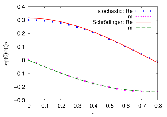
Figure 3: Real and imaginary part of the unequal-time two-point correlation function for the quantum anharmonic oscillator as a function of real time $t$. The results obtained from stochastic quantization agree to very good accuracy to those obtained from directly solving the Schrödinger equation.

5.1 Short-time evolution: Thermal fixed point

We consider an interacting scalar theory with classical action (58), where

$$V(\varphi)=\frac{1}{2}m^{2}\varphi^{2}+\frac{\lambda}{4!}\varphi^{4}\,,$$ (64)

in zero spatial dimension. The Schrödinger equation for the corresponding quantum anharmonic oscillator can be solved numerically by diagonalization of the Hamiltonian. We use the occupation number representation and truncate the Hilbert space keeping 32 dimensions corresponding to the lowest occupation numbers. Exponentiation of the diagonalized Hamiltonian yields the time translation operator, which may be used for real as well as complex times. We checked that the results are insensitive to an enlargement of the truncation dimension. This is compared to the results obtained from stochastic quantization by solving the Langevin dynamics according to (31). In the following all quantities will be given in appropriate units of the mass parameter $m$. We first perform simulations in thermal equilibrium, in which case the time contour extends along the imaginary axis to the inverse temperature $\beta$ (see Fig. 2). Non-equilibrium is considered in Sec. 5.3.

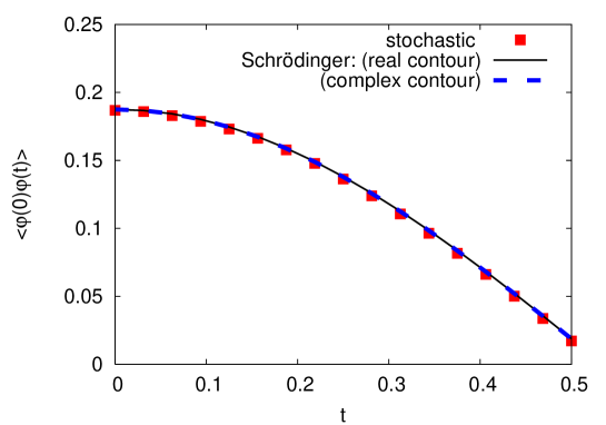
Figure 4: Similar evolution as in Figs. 3 but for much stronger coupling $\lambda=96$ and $\beta=1$.

Fig. 3 shows the two-point correlation function $\langle\varphi(0)\varphi(t)\rangle_{\eta}$ as a function of real time $t$ for $\lambda=24$ and $\beta=1$. The real-time extent of the contour is $t_{\rm final}=0.8$, such that the upper branch has a tilt of $0.01\beta$ and the lower branch has a tilt of $0.99\beta$. Square symbols denote the results from stochastic quantization for the real part of the two-pint function and crosses for the imaginary part, respectively. For comparison the corresponding results from the Schrödinger equation are given, which agree well.

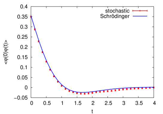
Figure 5: Similar evolution as in Figs. 3 but for smaller temperature ($\beta=8$ and $\lambda=6$) on an isosceles triangle contour.

Fig. 4 shows the real part of the two-point correlation function as a function of real time $t$, where we employ a much stronger coupling $\lambda=96$ and $\beta=1$. Square symbols denote the results from stochastic quantization. Here the real-time extent of the time contour is $t_{\rm final}=0.5$. The upper branch of the contour has a tilt of $0.001\beta$ with respect to the real-time axis, so it is almost horizontal and, therefore, realizes to high accuracy a real-time contour. For comparison results from the Schrödinger equation are displayed as well. The solid line corresponds to Minkowski time evolution (”real contour”), whereas the dashed line gives the results for those complex times with small imaginary part as employed in the stochastic quantization simulations (”complex contour”). They all agree well. We fit the time evolution to

$$\langle\varphi(0)\varphi(t)\rangle=a\cos\left(\omega\,{\rm Re}t\right)e^{-\gamma{\rm Re}t}\,,$$ (65)

which allows us to extract characteristic damping times. We find from the stochastic quantization simulation $\gamma/\omega=0.018$ and from the Schrödinger equation $\gamma/\omega=0.013$ (Minkowski) and $\gamma/\omega=0.014$ on the contour. The frequency is always $\omega=2.95$.

Fig. 5 shows a time evolution for smaller temperature with $\beta=8$ and $\lambda=6$. The real-time extent of the contour is $t_{\rm final}=4$. Using the fit (65) we find from the stochastic quantization simulation $\gamma/\omega=0.92$ and from the Hamiltonian diagonalization method $\gamma/\omega=1.0$ on the contour. The frequency is $\omega=1.4$.

Fig. 6 verifies the validity of the Dyson-Schwinger identity (52) for various real-time values. We use the parameters $\lambda=24$ and $\beta=1$. The real-time extent of the contour is $t_{\rm final}=1$ with 32 points in total on the (isosceles triangle) contour. Plotted is the Langevin-time evolution of the LHS and the RHS of the equation

$$\sum_{\bar{t}}G^{-1}_{0,t\bar{t}}\langle\varphi_{\bar{t}}\varphi_{t^{\prime}}\rangle-\delta_{tt^{\prime}}=-i\frac{\lambda}{3!}\langle\varphi_{t}\varphi_{t}\varphi_{t}\varphi_{t^{\prime}}\rangle\,,$$ (66)

where $G^{-1}_{0,t\bar{t}}$ is the inverse propagator (59) of the free theory. One observes that at sufficiently late Langevin times both sides agree to very good accuracy. In particular, one sees that equal-time values at different real times agree, which has to be the case for the time translation invariant thermal solution.

Figure 6: Shown is the Langevin-time evolution of the two-point function and four-point function given by the LHS and RHS of the Dyson-Schwinger identity (66). The curves are for fixed real-time values. At sufficiently late Langevin-time they agree to very good accuracy, thus becoming related by the Dyson-Schwinger equation.

5.2 Long-time evolution: Non-unitary fixed points

We observed above that stochastic quantization can describe the real-time evolution very accurately for short times. However, when the real-time extent of the lattice is enlarged the stochastic updating may not converge to the correct solution. As an example, Fig. 7 shows the two-point correlation function as a function of real time $t$ for $\lambda=24$ and $\beta=1$, i.e. for the parameters of Fig. 3. From that figure we have seen that for a real-time lattice with $t_{\rm final}=0.8$ there is excellent agreement of stochastic quantization and Schrödinger equation results. Correspondingly, Fig. 7 exhibits a constant real part and a vanishing imaginary part of the equal-time correlator in thermal equilibrium for $t_{\rm final}=0.8$. However, doubling the extent of the contour leads to a qualitatively different behavior as indicated by the cross symbols of Fig. 3. This difference persists also on finer real-time grids. The non-vanishing imaginary part of the equal-time correlator and the loss of time-translation invariance reflects a non-unitary time evolution.

Figure 7: Real and imaginary part of the equal-time correlator as a function of time (index of lattice site along the time-contour) for the parameters ($\lambda=24$ and $\beta=1$) as well as the contour of Fig. 3. Compared are two simulations where the real-time extent of the lattice differs by a factor of two. The larger lattice leads to a qualitatively different, non-unitary behavior.

The properties of these non-unitary fixed point solutions depend on the details of the time contour. This is in contrast to the universal properties of the thermal solution. As an example, Fig. 8 shows the equal-time two point function for same $\lambda=24$ and $\beta=1$ as in Fig. 7, however, with different contour geometry (isosceles triangle). For $t_{\rm final}=1$ one still observes the thermal fixed point solution, whose properties agree very well with those obtained from lattices with smaller $t_{\rm final}$. Stretching the temporal extent of the contour to $t_{\rm final}=2$ the Langevin dynamics converges to a non-unitary fixed point as one can see from Fig. 8. The detailed properties of this fixed point differ from those shown in Fig. 7.

Figure 8: Similar evolution as in Fig. 7, but on an isosceles triangle contour. While the thermal solution obtained for $t_{\rm final}=1$ does not depend on the contour details (see also Fig. 6), the properties of the non-unitary fixed point obtained for $t_{\rm final}=2$ are contour dependent (see also Figs. 9 and 10).

In Fig. 6 we have shown how the propagator fulfils for the thermal fixed point the corresponding Dyson-Schwinger identity. According to the results of Sec. 4 any fixed point solution has to fulfil the same properly symmetrized Dyson-Schwinger identities. For instance, the identity (52) reads

$$\sum_{\bar{t}}G^{-1}_{0,t\bar{t}}\langle\varphi_{\bar{t}}\varphi_{t^{\prime}}\rangle+\sum_{\bar{t}}G^{-1}_{0,t^{\prime}\bar{t}}\langle\varphi_{\bar{t}}\varphi_{t}\rangle+-2\delta_{tt^{\prime}}=-i\frac{\lambda}{3!}\langle\varphi_{t}\varphi_{t}\varphi_{t}\varphi_{t^{\prime}}\rangle-i\frac{\lambda}{3!}\langle\varphi_{t}\varphi_{t^{\prime}}\varphi_{t^{\prime}}\varphi_{t^{\prime}}\rangle\,.$$ (67)

We display the LHS and the RHS of this equation as a function of Langevin-time in Fig. 9. Indeed, one observes that the symmetrized Dyson-Schwinger equation (52) holds within statistical errors at late Langevin-time for the non-unitary solution. In Fig. 10 we check Eq. (66), which is the non-symmetrized version of Eq. (52). Here the discrepancy we find for the non-unitary fixed point is greater than the statistical error. In contrast, the thermal fixed point solution respects, of course, both Eqs. (67) and (66) as required by any physical solution for the underlying quantum field theory.

Figure 9: The left-hand-side (LHS) and right-hand-side (RHS) of the Dyson-Schwinger equation (67) for the non-unitary fixed point, which agree well at late Langevin time. Contrary to the properties of the thermal fixed point (see Fig. 6), the $(0,0)$ and $(t,t)$ components are not equal, which reflects the loss of time translation invariance.

Figure 10: The left-hand-side (LHS) and right-hand-side (RHS) of equation (66), showing a discrepancy beyond the statistical error.

5.3 Non-equilibrium dynamics

Non-equilibrium dynamics can be described by the generating functional for correlation functions [16]:

$$Z[J;\rho]={\rm Tr}\left\{\rho\,T_{\mathcal{C}}\,e^{i\int_{\mathcal{C}}\!J(x)\Phi(x)}\right\}$$ (68)

$$= \int{\rm d}\varphi_{1}{\rm d}\varphi_{2}\,\rho(\varphi_{1},\varphi_{2})\int\limits_{\varphi_{1}}^{\varphi_{2}}D^{\prime}\varphi\,e^{i\int_{\mathcal{C}}\left(L(x)+J(x)\varphi(x)\right)}.\,\,$$

The path integral (68) displays the quantum fluctuations for a theory with Lagrangian $L$, and the statistical fluctuations encoded in the weighted average with the initial-time (non-thermal) density matrix $\rho(\varphi_{1},\varphi_{2})$. Here $T_{\mathcal{C}}$ denotes contour time ordering along a closed path $\mathcal{C}$ starting at $t\equiv x^{0}=0$ with $\int_{\mathcal{C}}\equiv\int_{\mathcal{C}}{\rm d}x^{0}\int{\rm d}^{d}x$. This corresponds to usual time ordering along the forward piece $\mathcal{C}_{+}$, and anti-temporal ordering on the backward piece $\mathcal{C}_{-}$. Denoting fields on $\mathcal{C}_{+}$ by $\varphi_{+}(x)$ and on $\mathcal{C}_{-}$ by $\varphi_{-}(x)$, the initial fields are fixed by $\varphi_{1}({\mathbf{x}})=\varphi_{+}(t=0,{\mathbf{x}})$ and $\varphi_{2}({\mathbf{x}})=\varphi_{-}(t=0,{\mathbf{x}})$. Non-equilibrium correlation functions are obtained by functional differentiation and setting $J=0$.

With this notation the expectation value of a real-time observable ${\cal A}(\varphi)$ can be written as

$$\left\langle{{\cal A}(\varphi)}\right\rangle = \int{\rm d}\varphi_{1}{\rm d}\varphi_{2}\,\rho(\varphi_{1},\varphi_{2})\int_{\varphi_{+}(0)=\varphi_{1}}^{\varphi_{-}(0)=\varphi_{2}}D^{\prime}\varphi_{-}D^{\prime}\varphi_{+}e^{iS[\varphi_{+}]-iS[\varphi_{-}]}{\cal A}(\varphi_{+})$$ (69)

$$= \int D\varphi_{-}D\varphi_{+}e^{iS_{\rho}[\varphi_{+},\varphi_{-}]}{\cal A}(\varphi_{+})\,.$$ (70)

Here $S_{\rho}$ contains the actions on both contour branches as well as the density operator. In the following we consider Gaussian initial density matrices for which, neglecting all space dependence for simplicity, the most general $S_{\rho}$ reads [16]

$$S_{\rho}[\varphi_{+},\varphi_{-}] = S[\varphi_{+}]-S[\varphi_{-}]-\frac{i}{a_{t}}S_{0}(\varphi_{+}(t=0),\varphi_{-}(t=0)]\,,$$ (71)

$$S_{0}[\varphi_{+},\varphi_{-}] = i\dot{\phi}(\varphi_{+}-\varphi_{-})-\frac{\sigma^{2}+1}{8\xi^{2}}\left((\varphi_{+}-\phi)^{2}+(\varphi_{-}-\phi)^{2}\right)$$ (72)

$$+ \frac{i\eta}{2\xi}\left((\varphi_{+}-\phi)^{2}-(\varphi_{-}-\phi)^{2}\right)$$

$$+ \frac{\sigma^{2}-1}{4\xi^{2}}(\varphi_{+}-\phi)(\varphi_{-}-\phi)\,.$$

The real parameters $\phi$, $\dot{\phi}$, $\sigma$, $\xi$, $\eta$ determine a complete set of independent initial one-point and two-point correlation functions:

$$\phi = \left\langle{\varphi(t=0)}\right\rangle\quad,\qquad\dot{\phi}\,=\,\left\langle{\dot{\varphi}(t=0)}\right\rangle\,,$$

$$\xi^{2} = \left\langle{\varphi(t=0)\varphi(t=0)}\right\rangle_{c}\,,$$

$$\eta\xi = \frac{1}{2}\left\langle{\dot{\varphi}(t=0)\varphi(t=0)+\varphi(t=0)\dot{\varphi}(t=0)}\right\rangle_{c}\,,$$

$$\eta^{2}+\frac{\sigma^{2}}{4\xi^{2}} = \left\langle{\dot{\varphi}(t=0)\dot{\varphi}(t=0)}\right\rangle_{c}\,.$$ (73)

Starting from a given initial density matrix the nonequilibrium simulation is carried out using the Langevin equation (31) with the action replaced by (71), i.e.

$$\varphi_{\pm}^{\prime}(x)=\varphi_{\pm}(x)+i\,\epsilon\,\frac{\delta S_{\rho}[\varphi_{+},\varphi_{-}]}{\delta\varphi_{\pm}(x)}+\sqrt{\epsilon}\,\eta_{\pm}(x)\,,$$ (74)

updating all the points including $\varphi_{\pm}(t=0)$.

As an example, Fig. 11 shows the time evolution of the expectation value $\left\langle{\varphi(t)}\right\rangle$ as a function of time, all in units of the mass parameter $m$ of equation (64). Here the coupling is $\lambda=1$ for zero spatial dimension. The initial conditions are $\left\langle{\varphi(t=0)}\right\rangle=1$, $\left\langle{\varphi(t=0)\varphi(t=0)}\right\rangle_{c}=1$, $\left\langle{\dot{\varphi}(t=0)\dot{\varphi}(t=0)}\right\rangle_{c}=0.25$ and zero for the remaining quantities of (73). The time contour is tilted with $5\%$ slope, which is denoted as complex contour in Fig. 11. Results using stochastic quantization are given for three different lengths of the real-time extent of the contour ($t_{\rm final}=2,1$ and $0.5$). For comparison we also show the results of the numerical solution of the corresponding Schrödinger equation (see Sec. 5.1) for real times as well as for the complex times on the tilted contour. This also illustrates the contour dependence of the results. One observes that the stochastic quantization algorithm produces accurate results on the contour for sufficiently short real-time extent. Like for the thermal equilibrium results of Sec. 5.1, we find that it becomes inaccurate for late-time evolution.

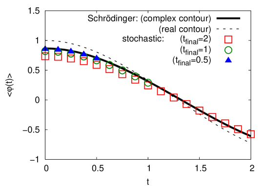
Figure 11: Non-equilibrium time evolution of the field expectation value as a function of time. Shown are results for different real-time extents of the lattice. Shorter $t_{\rm final}$ lead to improved agreement with results of the Schrödinger equation on the employed complex contour.

6 Accuracy tests II: nonabelian gauge theory

In the following we perform a similar investigation for $SU(2)$ gauge theory as done above for the scalar theory. Though some aspects of the application of real-time stochastic quantization are comparable, we will find that there are crucial additional restrictions concerning its range of validity for nonabelian gauge theories.

The equation for the Langevin evolution is given by Eq. (45) for the action (43), where we employ the approximation that $g_{0}=g_{s}$. We use the $U=a{\bf 1}+ib_{a}\sigma^{a},\ a^{2}+b^{2}_{a}=1$ representation for $SU(2)$ matrices. For $SL(2)$, the representation with the same constraint can be used, but the parameters $a$ and $b_{a}$ are no longer real. We expand the exponential to first order in $\epsilon$, which means we must include the square of the noise term, which is proportional to unity. The evolution equation then reads

$$U^{\prime}_{x,\mu} = \left(a{\bf 1}+i\sigma_{a}\left(\epsilon\,iD_{x\mu a}S[U]+\sqrt{\epsilon}\,\eta_{x\mu a}\right)\right)U_{x,\mu}\,.$$ (75)

To stay in group space the constant $a$ is calculated from the constraint $a^{2}+b_{a}^{2}=1$ of the matrix transforming $U_{x,\mu}$.

As the starting configuration for the Langevin-time evolution we take all link variables equal to unity. Typically we employ $1/\gamma=a_{t}/a_{s}=0.01-0.5$. We use lattices of spatial size $N^{3}=4^{3}$. The Langevin step used is $\sim 10^{-6}$. All quantities are given in units of $a_{s}$. The triangle contour of Fig. 2 is used, with $\tau_{+}$ being the imaginary extent of the contour on the forward part and $\tau_{-}$ on the backward part. We calculate thermal distributions, with inverse temperature $\tau_{+}+\tau_{-}=4$.

Figure 12: The spatial plaquette average as a function of Langevin time. Shown are results for different complex contours. Here $\alpha=0$ corresponds to a contour with an infinite extent along the real-time axis, while $\alpha=\pi/2$ denotes the Euclidean contour. The longer the real-time component of the contour the less accurately the thermal solution is reproduced.

Fig. 12 shows the Langevin-time evolution of the spatial plaquette average. The solid line shows the result for vanishing real-time extent, i.e. for a Euclidean contour. The different dashed curves correspond to results for complex contours on isosceles triangles ($\tau_{+}=\tau_{-}=2$) each having a different tilt $\alpha$ with respect to the real-time axis. Here $\alpha=0$ would correspond to an infinite extent along the real axis. One observes that with increased real-time extent or smaller tilt $\alpha$ the correct thermal solution is approached less accurately.

In particular, it is only approached at intermediate Langevin-times, irrespective of the details of the non-vanishing real-part of the contour. This aspect differs from the scalar case where short real-time extents lead to stable thermal solutions. For the nonabelian gauge theory the correct thermal fixed point is approached at first. However, it is not stable and the Langevin flow exhibits a crossover to another (stable) fixed point. The fact that the thermal solution is not a true fixed point for non-Euclidean contours can be seen by monitoring for example $\left\langle\textrm{Im}(i\textrm{Tr}(U_{x,\mu}\sigma^{a}))^{2}\right\rangle$, which is zero for $SU(2)$ matrices in the Euclidean theory. It is found to grow exponentially while observables of the original $SU(2)$ theory such as the plaquette average still approach the thermal solution.

Figure 13: The Langevin-time $\vartheta_{\rm crossover}$ for the crossover away from the approximate thermal solution to another fixed point. (See Fig. 12.) It is displayed as a function of ${\rm tan}\alpha$ for various time contours. Contours with different real-time extent, but with the same $\tau+$ are connected with a line.

This is quantified in Fig. 13, where the Langevin-time $\vartheta_{\rm crossover}$, at about which the crossover from the approximate thermal solution to another fixed point occurs, is given for various time contours. One observes that the time of the crossover is mostly dependent on the angle of the slope of the contour. Connecting points with the same $\tau_{+}$, one sees that $\theta_{\rm crossover}$ is approximately proportional to the logarithm of the tangent of the tilt of the contour. Here $\vartheta_{\rm crossover}$ was measured on $N_{t}=16$ lattices, using $\approx 5$ runs per parameters.

Figure 14: The spatial plaquette averages as a function of the index of lattice sites along the time-contour. One observes that it is time translation invariant to rather good accuracy for the approximate thermal fixed point, while it is not for the non-unitary fixed point.

In Fig. 14 the spatial plaquette average is shown as a function of the index of lattice sites along the time-contour. While the Langevin-time evolution approaches the thermal solution it is time translation invariant to rather good accuracy. The observed small discrepancy is decreasing with Langevin-time while the system stays close to the approximate thermal solution. In contrast, for the stable fixed point at late Langevin-time the plaquette averages are not time translation invariant along the contour — at least for the finite Langevin-times for which we followed the evolution. Here we employed a contour with $\tau_{+}=0.5$ and $\tau_{-}=3.5$ with $a_{t}/a_{s}=0.03$ and $N_{t}=20$ from an average over 10 runs. The real-time evolution near the thermal solution has been averaged over Langevin time $0.75<\vartheta<1.25$, for the non-unitary fixed point it has been averaged over $3.75<\vartheta<4.25$.

Figure 15: Numerical check of the Dyson-Schwinger equation for a spatial plaquette variable. Displayed are separately the LHS and the RHS of (57).

As is shown is Sec. 4.2, all converging solutions of the stochastic dynamics method fulfil the same infinite set of (symmetrized) Dyson-Schwinger identities of the quantum field theory. This is remarkable in view of the different “physical” and “unphysical” solutions that are observed. In Fig. 15 this is visualized for the example of the Dyson-Schwinger equation for a spatial plaquette variable. Plotted are separately the LHS and the RHS of the Dyson-Schwinger equation (57) for the plaquette (see also Fig. 1). The plot displays the respective LHS and RHS as a function of Langevin-time. The flow with Langevin-time quickly leads to a rather accurate agreement of both sides such that the Dyson-Schwinger equation is fulfilled. However, after some Langevin-time they start deviating again, finally leading to another stationary value where the LHS and RHS agree to reasonable accuracy. Here the fluctuations of measured quantities of the system are much bigger. This is indicated by the given typical statistical error bars, with a comparably huge statistical error for the late Langevin-time evolution. We used median averaging for the right hand side of the equations. For the contour we employ $\tau_{+}=\tau_{-}=2$ with $N_{t}=8$ and $a_{t}/a_{s}=0.25$.

7 Conclusions

The motivation for this paper is the question of making real-time, nonequilibrium quantum field theory amenable to numerical simulations from first principles. This would not only boost our knowledge directly, it would also allow better testing of approximate analytical tools. This concerns, in particular, strongly interacting theories such as QCD, where reliable analytical approximations are difficult to find at phenomenologically relevant energies. Despite its importance research on real-time lattice gauge theory is still in its infancies. It has been a delicate problem and the various attempts based on reweighting or on Euclidean simulations have encountered major difficulties. Our aim here was to study the applicability of stochastic quantization to real-time, nonequilibrium problems. This method does, a priori, not involve any reweighting, nor redefinition of the Minkowski dynamics in terms of an associated Euclidean one.

For setting up the procedure, both for scalar and for nonabelian gauge theory, we started from a five-dimensional classical Hamiltonian dynamics supplemented by a stochastic description and correctly accounting for the symmetries of the models. We then showed that the fixed points of the Langevin (fifth-time) dynamics fulfil the infinite set of Dyson-Schwinger equations associated with the respective quantum theory. We established in this way a set of identities to be fulfilled by the expectation values. These general results both allow checks of the simulations and suggest means to understand convergence and metastability problems.

In the second part we undertook a numerical study of the real-time stochastic quantization approach applied to scalar and $SU(2)$ gauge theory as a paradigmatic Yang Mills model. The main aim being to understand the problems of, and to develop means to control the method. Beyond varying the parameters of the implementation we also worked on various realizations of nonequilibrium and of non-zero temperature problems, which correspondingly define various integration contours. Our findings can be summarized as follows (both for scalar and Yang Mills fields, unless explicitely distinguished):

- Instabilities of the Langevin dynamics are controllable: if the Langevin step size is chosen small enough run-away trajectories are rather seldom and the results do not suffer from discarding them.

- Tilting the integration contour in the complex plane is a gauge invariant way to improve both the convergence and the accuracy of the results. The physical effect of this tilt can be understood from exact results (e.g., Schrödinger equation for the anharmonic oscillator) and small tilts can therefore be used in the simulation.

- Short real-time physics in thermal equilibrium can be reproduced reasonably well if the length of the real time contour is small on the scale of the inverse temperature $\beta$, the details depending also on other parameters as explained in the main text. The Langevin flow is here dominated by a thermal fixed point which fulfils the unsymmetrized Dyson-Schwinger identities and describes a physical solution. This fixed point is stable for the scalar theory while it is metastable for the gauge theory, its life-time depending then on the contour and the other parameters of the problem.

- For longer contours the boundary conditions in physical time do not seem to constrain enough the Langevin flow and the life-time of the thermal (physical) fixed point decreases (for gauge theory), or the fixed point becomes fully unstable (for scalar theory). A second, apparently stable fixed point develops for large Langevin times. This latter fixed point represents an unphysical, non-unitary regime, to be recognized by non-translational invariant expectation functions and violation of the unsymmetrized Dyson-Schwinger identities (while the symmetrized ones are still satisfied, indicating convergence).

- For nonequilibrium problems similar observations hold. For the scalar model all these findings have been checked by comparing with results from a numerical solution of the corresponding Schrödinger equation.

In view of these results we conclude that the Langevin approach can be used in direct numerical simulations of Minkowski theories, including Yang Mills theory, if a number of (rather severe) restrictions are observed. In those situations where physical solutions become unstable other, unphysical solutions will develop, but tests for differentiating them can typically be devised and applied. We did not try to optimize so far. The method allows for quite some flexibility as to which quantities are chosen to define the stochastic process, or introducing a stochastic reweighting. This is work in progress.

Part of the numerical calculations have been performed on HELICS of the IWR Heidelberg.

References

- [1]
- [2] U. W. Heinz, AIP Conf. Proc. 739 (2005) 163
- [3] J.D. Gunton, M. San Miguel and P. S. Sahni, in “Phase Transitions and Critical Phenomena, v. 8”, ed. C. Domb and J. L. Lebowitz, Academic Press (1983).
- [4] T. R. Miller and M. C. Ogilvie, Phys. Lett. B 488 (2000) 313. A. Bazavov, B. A. Berg and A. Velytsky, Int. J. Mod. Phys. A 20 (2005) 3459; Phys. Rev. D 74, 014501 (2006). E. T. Tomboulis and A. Velytsky, Phys. Rev. D 72, 074509 (2005).
- [5] G. Parisi and Y.-S. Wu , Sci. Sin. 24 (1981) 483. For reviews see E. Seiler, Schladming (1984) 259. P. H. Damgaard and H. Hüffel, Phys. Rept. 152 (1987) 227.
- [6] E. Seiler, I. O. Stamatescu and D. Zwanziger, Nucl. Phys. B 239 (1984) 177; Nucl. Phys. B 239 (1984) 201. G. G. Batrouni et al, Phys. Rev. D 32 (1985) 2736.
- [7] J. Berges and I. O. Stamatescu, Phys. Rev. Lett. 95 (2005) 202003
- [8] J. R. Klauder, in “Recent developments in High Energy Physics,” ed. H. Mitter and C. B. Lang, Springer (1983); Phys. Rev. A 29 (1984) 2036. G. Parisi, Phys. Lett. B 131 (1983) 393. For a review see K. Okano, L. Schulke and B. Zheng, Prog. Theor. Phys. Suppl. 111 (1993) 313.
- [9] H. Hüffel and H. Rumpf, Phys. Lett. B 148 (1984) 104. E. Gozzi, Phys. Lett. B 150 (1985) 119. D. J. E. Callaway et al, Nucl. Phys. B 262, 19 (1985). H. Nakazato and Y. Yamanaka, Phys. Rev. D 34 (1986) 492. H. Okamoto et al, Nucl. Phys. B 324 (1989) 684.
- [10] H. Hüffel and P. V. Landshoff, Nucl. Phys. B 260 (1985) 545.
- [11] J. Flower, S. W. Otto and S. Callahan, Phys. Rev. D 34 (1986) 598. J. Ambjorn, M. Flensburg and C. Peterson, Nucl. Phys. B 275 (1986) 375.
- [12] F. Karsch and H. W. Wyld, Phys. Rev. Lett. 55 (1985) 2242. H. Gausterer and J. R. Klauder, Phys. Lett. B 164 (1985) 127; Phys. Rev. Lett. 56 (1986) 306; Phys. Rev. D 33 (1986) 3678. E. M. Ilgenfritz, Phys. Lett. B 181 (1986) 327. J. Ambjorn and S. K. Yang, Nucl. Phys. B 275 (1986) 18. N. Bilic, H. Gausterer and S. Sanielevici, Phys. Lett. B 198 (1987) 235; Phys. Rev. D 37 (1988) 3684. C. Adami and S. E. Koonin, Phys. Rev. C 63 (2001) 034319. C. W. Bernard and V. M. Savage, Phys. Rev. D 64 (2001) 085010.
- [13] J. Klauder and W. Petersen, J. Stat. Ph. 39 (1985) 53. J. Ambjorn and S. K. Yang, Phys. Lett. B 165 (1985) 140. T. Matsui and A. Nakamura, Phys. Lett. B 194 (1987) 262. K. Okano, L. Schulke and B. Zheng, Phys. Lett. B 258 (1991) 421. L. L. Salcedo, Phys. Lett. B 305 (1993) 125. K. Fujimura et al, Nucl. Phys. B 424 (1994) 675. H. Gausterer, J. Phys. A 27 (1994) 1325.
- [14] See e.g. I. Montvay and G. Münster, “Quantum Fields on a Lattice”, Cambridge University Press (1997).
- [15] S. Xue, Phys. Lett. B 180 (1986) 275.
- [16] J. Berges, “Introduction to nonequilibrium quantum field theory,” AIP Conf. Proc. 739 (2005) 3 [arXiv:hep-ph/0409233], and references therein.