Color Screening, Casimir Scaling, and Domain Structure in G(2) and SU(N) Gauge Theories

Abstract

We argue that screening of higher-representation color charges by gluons implies a domain structure in the vacuum state of non-abelian gauge theories, with the color magnetic flux in each domain quantized in units corresponding to the gauge group center. Casimir scaling of string tensions at intermediate distances results from random spatial variations in the color magnetic flux within each domain. The exceptional G(2) gauge group is an example rather than an exception to this picture, although for G(2) there is only one type of vacuum domain, corresponding to the single element of the gauge group center. We present some numerical results for G(2) intermediate string tensions and Polyakov lines, as well as results for certain gauge-dependent projected quantities. In this context, we discuss critically the idea of projecting link variables to a subgroup of the gauge group. It is argued that such projections are useful only when the representation-dependence of the string tension, at some distance scale, is given by the representation of the subgroup.

I Introduction

Over the past decade, a great deal of numerical evidence has been obtained in favor of the center vortex confinement mechanism (for reviews, cf. refs. review and michael ). According to this proposal, the asymptotic string tension of a pure non-abelian gauge theory results from random fluctuations in the number of center vortices linked to Wilson loops. It is sometimes claimed that gauge theory based on the exceptional group G(2) is a counterexample to the vortex mechanism, in that the theory based on G(2) demonstrates the possibility of having “confinement without the center” Pepe1 . This claim has two questionable elements. In the first place, the asymptotic string tension of G(2) gauge theory is zero, in perfect accord with the vortex proposal. No center vortices means no asymptotic string tension. From this point of view G(2) gauge theory is an example of, rather than a counterexample to, the importance of vortices. The question of whether G(2) gauge theory is nonetheless confining then depends on what one means by the word “confinement”. This is a basically a semantic issue, but for the sake of clarity we will explain our view below. The second point is that G(2), like any group, does have a center subgroup. This may seem like a quibble, since the center of G(2) is trivial, consisting only of the identity element. We will argue, however, that this group element has an important role to play, not only in G(2) but perhaps also in SU(N) gauge theories, in the classification of non-trival vacuum structures.

We begin with a discussion of the term “confinement”, which is used in the literature in several inequivalent ways:

1. Confinement refers to electric flux-tube formation, and a linear static quark potential.

2. Confinement means the absence of color-electrically charged particle states in the spectrum.

3. Confinement is the existence of a mass gap in a gauge field theory.

We prefer the first of these options. Real QCD, according to this definition, confines at intermediate but not at large distance scales, since electric flux tubes break, the static potential goes flat, and excited hadronic states with string-like configurations are only metastable. For this reason we use the term “temporary confinement” to describe the situation in real QCD with light quarks. Most discussions, however, do not make such a distinction, and apply the label “confinement” to real QCD without any qualification. In that case, to conform to common usage, why not adopt the second or third definitions? Our reason is that this choice would force us to also describe many other theories as “confining” which are not normally considered so, and which (unlike real QCD) have nothing at all to do with flux tube formation and confining potentials.

As one example, let us consider an electric superconductor, or, in its relativistic version, the abelian Higgs model. In this theory, any external electric charge is screened immediately by the condensate. There is a mass gap, and asymptotic particle states are all electrically neutral. If definitions (2) and/or (3) define confinement, then the abelian Higgs model is surely confining. But this contradicts standard usage in the literature, where confinement of electric charge is often identified with a dual (i.e. magnetic) abelian Higgs model, while the ordinary abelian Higgs model is identified with confinement of magnetic, not electric, charge.

A second example along the same lines is an electrically charged plasma. In response to an external charge, the plasma rearranges itself to screen out the field (and hence the charge) of the probe. Since all probe charges are neutralized, and all Coulombic fields are Debye screened, an electrical plasma could also be taken, according to definition (2), as a confining system.

Our third example is an SU(2) gauge-Higgs theory with a pair of Higgs fields in the adjoint representation. In this case there are two distinct massive phases of the system, characterized by an asymptotic string tension which is non-zero in one phase, and zero in the other. We have every right, in this theory, to distinguish between the Confinement phase and the Higgs phase. But definitions (2) and (3) allow no such distinction. Both phases, according to these definitions (and according to the Fredenhagen-Marcu criterion FM ) are equally confining. Again, we feel that this is an abuse of the term “confinement”.

Our point is that consistent application of any of the three suggested definitions does at least some violence to common usage. According to our preferred terminology, i.e. option (1), both real QCD and G(2) gauge theory are examples of only “temporary” confinement. The other options, in our opinion, are worse. We do not think that electric superconductors, electrical plasmas, and gauge systems which are clearly in a Higgs phase, should be described by a term which is so often and so generally associated with electric flux tubes and a linear potential.

Of course, the serious question to be addressed is not whether or not to refer to G(2) gauge theory as confining; at the end of the day this is only a matter of words. The real challenge which is posed by G(2) gauge theory, in our opinion, is the fact that this theory has a non-vanishing string tension for the static quark potential over some finite range of distances, intermediate between the breakdown of perturbation theory and the onset of color screening. Where does that string tension come from, if not from vortices? This question has, in fact, a much broader context. In connection with SU(N) gauge theories, we have emphasized many times in the past (beginning with ref. Cas ) that the dependence of the string tension on the color group representation of the static quarks falls into two general categories, depending on distance scale:

1. The Casimir Scaling Region $-$ At intermediate distances, the string tension of the static quark potential, for quarks in group representation $r$, is approximately proportional to the quadratic Casimir $C_{r}$ of the representation, i.e.

   $$\sigma_{r}\approx\frac{C_{r}}{C_{F}}\sigma_{F}$$ (1)

   where $F$ denotes the fundamental, defining representation. Thus, e.g., the string tension of quarks in the adjoint representation of SU(N) gauge theory is about twice as large as that of quarks in the fundamental representation.

2. The Asymptotic Region $-$ Asymptotically, due to color screening by gluons, the string tension depends only on the transformation properties of representation $r$ with respect to the center subgroup; i.e. on the N-ality $k_{r}$ in an SU(N) gauge theory:

   $$\sigma_{r}=\sigma(k_{r})$$ (2)

   where $\sigma(k)$ is the string tension of the lowest dimensional representation of SU(N) with N-ality $k$. These are known as the “k-string tensions.” The string tension of adjoint representation quarks in the asymptotic region is zero.

We have no reason to think that G(2) gauge theory differs from SU(N) gauge theories with respect to the intermediate/asymptotic behaviors of the string tension. First of all, there is certainly a linear static quark potential in an intermediate region (as we confirm by numerical simulations), and we think it likely that the representation dependence of the string tension at intermediate distances follows an approximate Casimir scaling law. Casimir scaling has not been checked numerically for G(2), but for the purposes of this article we will assume it to be true, pending future investigation. Secondly, all G(2) group representations transform in the same way with respect to the center subgroup, i.e. trivially, and all must have the same asymptotic string tension, namely zero, because of color screening by gluons. Therefore, the existence of a linear potential in G(2) is the subject of a broader question, relevant to any gauge group: If center vortices (or the absence of center vortices) explains the values of the asymptotic string tension, then what accounts for the linear static quark potential at intermediate distance scales, where the string tension depends on the quadratic Casimir of the gauge group, rather than the representation of the gauge group center?

In the next two sections we will present our answer to this question, which improves, in some crucial ways, on an old model introduced by two of the present authors, in collaboration with M. Faber ccv . We begin by asking (section II) what features, of a typical gauge field vacuum fluctuation, can possibly account for both Casimir scaling and color screening. We are led to postulate (in section III) a kind of domain structure in the vacuum, with magnetic flux in each domain quantized in units corresponding to the elements of the center subgroup, including the identity element. In section IV we present some lattice Monte Carlo results for G(2) gauge theory, which confirm (as expected) the existence of a string tension over some intermediate distance range. In section V we consider fixing the gauge in G(2) lattice gauge theory, so as to leave either an SU(3), $Z_{3}$, or SU(2) subgroup unfixed, together with a projection of the G(2) link variables to the associated subgroup. While there are some numerical successes with this procedure, suggestive of SU(3) or $Z_{3}$ or SU(2) “dominance” in G(2) gauge theory, in the end we were unable, at least thus far, to find any correlation between the projected observables and gauge-invariant observables. We think this failure makes a point which may also be relevant to, e.g., abelian projection in SU(N) theories: Projection to a subgroup is unlikely to be of much significance, unless the group representation-dependence of the string tension, at some distance scale, depends only on the representation of the subgroup. Section VI contains some concluding remarks.

II Casimir Scaling

Casimir scaling of string tensions is quite natural in non-abelian gauge theory. Consider a planar Wilson loop in group representation $r$. Take the loop to lie in, e.g., the $x-y$ plane at $z=t=0$, and imagine integrating over all links, in the functional integral, which do not lie in the plane, i.e.

$$W_{r}(C) = {1\over Z}\int DU_{\mu}(x,y,z,t)~{}\chi_{r}[U(C)]e^{-S_{W}}$$ (3)

$$= \int DU_{x}(x,y,0,0)DU_{y}(x,y,0,0)~{}\chi_{r}[U(C)]$$

$$\Bigl{\{}\int[DU_{x}DU_{y}]_{z~{}\mbox{\small and/or}~{}t\neq 0}$$

$$\int DU_{z}(x,y,z,t)DU_{t}(x,y,z,t)~{}e^{-S_{W}}\Bigr{\}}$$

$$= {1\over Z}\int DU_{x}(x,y)DU_{y}(x,y)~{}\chi_{r}[U(C)]$$

$$\times\exp\Bigl{[}-S_{eff}[U_{x},U_{y}]\Bigr{]}$$

where $\chi_{r}$ is the group character in representation $r$, and $U(C)$ the loop holonomy. Then the computation of the planar loop in $D=4$ dimensions, with the Wilson action $S_{W}$, is reduced to a computation in $D=2$ dimensions, with an effective action $S_{eff}$. This effective action can be regarded as the lattice regulation of some gauge-invariant $D=2$ dimensional continuum action $S_{eff}^{con}$. Although $S_{eff}^{con}$ is surely non-local, non-locality can, in some circumstances, be traded for a derivative expansion, so we have

$$S_{eff}^{con}=\int d^{2}x~{}\Bigl{(}a_{0}\mbox{Tr}[F^{2}]+a_{1}\mbox{Tr}[D_{\mu}FD_{\mu}F]+a_{2}\mbox{Tr}[(F^{4}]+...\Bigr{)}$$ (4)

where $F=F_{xy}$. Truncating $S_{eff}^{con}$ to the first term, which ought to be dominant at large scales, we obtain

$$W_{r}(C) \sim \frac{1}{Z}\int DA_{x}(x,y)DA_{y}(x,y)~{}\chi_{r}[U(C)]$$ (5)

$$\qquad\times\exp\left[-a_{0}\int d^{2}x~{}\mbox{Tr}[F^{2}]\right]$$

Since this is simply gauge theory in $D=2$ dimensions, the functional integral can be evaluated analytically, and the result is that the string tension is proportional to the quadratic Casimir $C_{r}$. It should be kept in mind, however, that the validity of the derivative expansion in (4) is an assumption. There might be some non-local terms in $S_{eff}$ which are not well represented by such an expansion.

The argument for an effective $D=2$ action can also be phrased in terms of the ground state wavefunctional $\Psi^{D}_{0}[A]$ of $D+1$ dimensional gauge theory in temporal gauge. It was originally suggested in ref. Me1 that for long-wavelength fluctations, the ground state could be approximated as

$$\Psi^{D}_{0}[A]\sim\exp\left[-\mu\int d^{D}x~{}\mbox{Tr}[F^{2}]\right]$$ (6)

In that case

$$W_{r}(C) = \langle\chi_{r}[U(C)]\rangle^{D=4}=\langle\Psi^{3}_{0}|\chi_{r}[U(C)]|\Psi^{3}\rangle$$ (7)

$$\sim \langle\chi_{r}[U(C)]\rangle^{D=3}=\langle\Psi^{2}_{0}|\chi_{r}[U(C)]|\Psi^{2}\rangle$$

$$\sim \langle\chi_{r}[U(C)]\rangle^{D=2}$$

and again the $D=4$ dimensional calculation has been reduced, in two steps, to the $D=2$ dimensional theory, where the string tensions are known to obey the Casimir scaling law. The argument hangs on the validity of the approximation (6). This approximation is supported by Hamiltonian strong-coupling lattice gauge theory, where the ground state can be calculated analytically Me2 , and it has also been checked numerically Me3 . Karabali, Kim, and Nair Nair have pioneered an approach in which the ground state wavefunctional $\Psi^{2}_{0}[A]$ of $D=2+1$ dimensional gauge theory can be calculated analytically in the continuum, as on the lattice, in powers of $1/g^{2}$, and according to these authors the leading term is again given by eq. (6). See also Leigh et al. Leigh and Freidel Freidel .

Returning to eq. (5), we note that what it really says is that on a $D=2$ slice of $D=4$ dimensions, the field strength of vacuum fluctuations is uncorrelated from one point to the next. This is because, in $D=2$ dimensions, there is no Bianchi identity constraining the field strengths, and, by going to an axial gauge, the integration over gauge potentials $A_{x},~{}A_{y}$ can be traded for an integration over the field strength $F_{xy}$. The absence of derivatives of $F$ in eq. (5) means that the field strengths fluctuate independently from point to point. This is, of course, absurd at short distance scales, and results from dropping the derivative terms in eq. (4). On the other hand, suppose that $F_{xy}$ has only finite-range correlations, with correlation length $l$ on the two-dimensional surface slice. In that case, dropping the derivative terms may be a reasonable approximation to $S_{eff}$ at scales larger than $l$, and Casimir scaling is obtained at large distances.

Regardless of the derivation, the essential point is the following: Casimir scaling is obtained if field strengths on a 2D slice of the 4D volume have only finite range correlations. Then the color magnetic fluxes in neighboring regions of area $l^{2}$ are uncorrelated, the effective long-range theory is D=2 dimensional gauge theory, and Casimir scaling is the natural consequence.

Once Casimir scaling gets started, the next question is why it ever ends; i.e. why the representation dependence suddenly switches from Casimir scaling to N-ality dependence. The conventional answer is based on energetics: As the flux tube gets longer, at some stage it is energetically favorable to pair create gluons from the vacuum. These gluons bind to each quark, and screen the quark color charge from representation $r$ to representation $r_{min}$ with the lowest dimensionality and the same N-ality as $r$. In particular, if $r_{min}$ is a singlet, then the flux tube breaks. Note that this means that the approximations (5) and (6), which imply Casimir scaling, must break down at sufficiently large distance scales (at least for $N_{colors}<\infty$).

While the energetics reasoning for color screening via gluons is surely correct, when we speak of the “pair creation” of gluons out the vacuum, we are using the language of Feynman diagrams, and describing, in terms of particle excitations, the response of the vacuum to a charged source. However, the path-integral itself is a sum over field configurations. When a Wilson loop at a given location is evaluated by Monte Carlo methods, the lattice configurations which are generated stochastically have no knowledge of the location of the Wilson loop being measured, and no clue of where gluon pair creation should take place. The Wilson loop is just treated as an observable probing typical vacuum fluctuations, not as a source term in the action. Nevertheless, the Monte Carlo evaluation must somehow arrive at the same answer that is deduced, on the basis of energetics, from the particle picture of string breaking. This leads us to ask the following question: What feature of a typical vacuum fluctuation can account for both Casimir scaling of string tensions at intermediate distances, and center-dependence at large distances? What we are asking for is a “field” explanation of screening, to complement the particle picture.

An important observation is that if the asymptotic string tension is to depend only on N-ality, then the response of a large Wilson loop to confining vacuum configurations must also depend only on the N-ality of the loop. Center vortices are the only known example of vacuum configurations which have this property. The confinement scenario associated with center vortices is very well known: random fluctuations in the number of vortices topologically linked to a Wilson loop explain both the existence and the N-ality dependence of the asymptotic string tension. Casimir scaling, on the other hand, seems to require short-range field strength correlations with no particular reference to the center subgroup. As Casimir scaling and N-ality dependence each have straightforward, but different explanations, the problem is to understand how both of these properties can emerge, in a lattice Monte Carlo simulation, from the same set of thermalized lattices.

III A Model of Vacuum Structure

Since Casimir scaling is an intermediate range phenomenon, while N-ality dependence is asymptotic, we suggest that the random spatial variations in field strength, required for Casimir scaling, are found in the interior of center vortices. These interior variations cannot be entirely random however; they are subject to the constraint that the total magnetic flux, as measured by loop holonomies, corresponds to an element of the gauge group center.

The picture we have in mind is indicated schematically in Figs. 1 and 2; these are cartoons of the vacuum in a 2D slice of the $D=4$ spacetime volume. The first figure is an impression of the vacuum in Yang-Mills theory, the second is for G(2) theory. Each circular domain is associated with a total flux corresponding to an element of the center subgroup. The domains may overlap, with the fields in the overlap regions being a superposition of the fields associated with each overlapping domain. In the SU(2) case there are two types of regions, corresponding to the two elements of the center subgroup. Regions associated with the $Z_{2}$ center element $z=-1$ are 2D slices of the usual thick center vortices, and the straight lines are projections to the 2D surface of the Dirac 3-volume associated with each vortex. But domains corresponding to the $z=1$ center element are also allowed; we see no reason to forbid them. Within each domain, the field strength fluctuates almost independently in sub-regions of area $l^{2}$, where $l$ is a correlation length for field-strength fluctuations, subject only to the weak constraint that the total magnetic flux in each domain corresponds to a center element of the gauge group. In the case of G(2) there is of course only one center element $z=1$ of the trivial $Z_{1}$ subgroup, and no Dirac volume, hence the difference in the two cartoons. This picture is sufficient to explain the N-ality dependence of loops which are large compared to the domain size, and Casimir scaling of loops which are small compared to the domain size.

Figure 1: A 2D slice of the D=4 Yang-Mills vacuum. Circular regions with (Dirac) lines correspond to $z=-1$ domains, circular regions without lines denote $z=+1$ domains.

Figure 2: A 2D slice of the D=4 vacuum of G(2) gauge theory. There is only one type of domain, corresponding to the single element of the center subgroup.

To support the last statement we return to an old model introduced in ref. ccv . In this model, it is assumed that the effect of a domain (2D cross-section of a vortex) on a planar Wilson loop holonomy is to multiply the holonomy by a group element

$$G(\alpha^{n},S)=S\exp[i\vec{\alpha^{n}}\cdot\vec{H}]S^{\dagger}$$ (8)

where the $\{H_{i}\}$ are generators of the Cartan subalgebra, $S$ is a random group element, $\vec{\alpha^{n}}$ depends on the location of the domain relative to the loop, and $n$ indicates the domain type. If the domain lies entirely within the planar area enclosed by the loop, then

$$\exp[i\vec{\alpha^{n}}\cdot\vec{H}]=z_{n}I$$ (9)

where

$$z_{n}=e^{2\pi in/N}\in Z_{N}$$ (10)

and $I$ is the unit matrix. At the other extreme, if the domain is entirely outside the planar area enclosed by the loop, then

$$\exp[i\vec{\alpha^{n}}\cdot\vec{H}]=I$$ (11)

For a Wilson loop in representation $r$, the average contribution from a domain will be

$${\large\cal G}_{r}[\alpha^{n}]I_{d_{r}} = \int dS~{}S\exp[i\vec{\alpha}^{n}\cdot\vec{H}]S^{\dagger}$$ (12)

$$= \frac{1}{d_{r}}\chi_{r}\Bigl{[}\exp[i\vec{\alpha}^{n}\cdot\vec{H}]\Bigr{]}I_{d_{r}}$$

where $d_{r}$ is the dimension of representation $r$, and $I_{d_{r}}$ is the unit matrix.

Consider, e.g., SU(2) lattice gauge theory, choosing $H=L_{3}$. The center subgroup is $Z_{2}$, and there are two types of domains, corresponding to $z_{0}=1$ and $z_{1}=-1$. Let $f_{1}$ represent the probability that the midpoint of a $z_{1}$ domain is located at any given plaquette in the plane of the loop, with $f_{0}$ the corresponding probability for a $z_{0}=1$ domain. Let us also make the drastic assumption that the probabilities of finding domains of either type centered at any two plaquettes $x$ and $y$ are independent. Obviously this “non-interaction” of domains is a huge over-simplification, but refinements can come later. If we make this assumption, then

$$\langle W_{j}(C)\rangle$$ (13)

$$\approx \prod_{x}\Bigl{\{}(1-f_{1}-f_{0})+f_{1}{\large\cal G}_{j}[\alpha^{1}_{C}(x)]+f_{0}{\large\cal G}_{j}[\alpha^{0}_{C}(x)]\Bigr{\}}W_{j}^{pert}(C)$$

$$= \exp\left[\sum_{x}\log\Bigl{\{}(1-f_{1}-f_{0})+f_{1}{\large\cal G}_{j}[\alpha^{1}_{C}(x)]\right.$$

$$\qquad\left.+f_{0}{\large\cal G}_{j}[\alpha^{0}_{C}(x)]\Bigr{\}}\right]W_{j}^{pert}(C)$$

where the product and sum over $x$ runs over all plaquette positions in the plane of the loop $C$, and $\alpha^{n}_{C}(x)$ depends on the position of the vortex midpoint $x$ relative to the location of loop $C$. The expression $W_{j}^{pert}(C)$ contains the short-distance, perturbative contribution to $W_{j}(C)$; this will just have a perimeter-law falloff.

To get the static potential, we consider loop $C$ to be a rectangular $R\times T$ contour with $T\gg R$. Then the contribution of the domains to the static potential is

$$V_{j}(R)=-\sum_{x=\infty}^{\infty}\log\Bigl{\{}(1-f_{1}-f_{0})+f_{1}{\large\cal G}_{j}[\alpha^{1}_{R}(x)]+f_{0}{\large\cal G}_{j}[\alpha^{0}_{R}(x)]\Bigr{\}}$$ (14)

where $x$ is now the distance from the middle of the vortex to one of the time-like sides of the Wilson loop. The question is what to use as an ansatz for $\alpha^{n}_{R}(x)$. One possibility was suggested in ref. ccv , but there the desired properties of the potential in the intermediate region, namely linearity and Casimir scaling, were approximate at best. We would like to improve on that old proposal.

Our improved ansatz is motivated by the idea that the magnetic flux in the interior of vortex domains fluctuates almost independently, in subregions of extension $l$, apart from the restriction that the total flux results in a center element. To estimate the effect of this restriction, consider a set of random numbers $\{F_{n}\},n=1,2,...,M$, whose probability distributions are independent apart from the condition that their sum must equal $2\pi$, i.e.

$$\langle Q[\{F_{n}\}]\rangle=\frac{\int\prod_{n}dF_{n}Q[\{F_{n}\}]e^{-\mu\sum_{n=1}^{M}F_{n}^{2}}\delta\left(\sum_{n=1}^{M}F_{n}-2\pi\right)}{\int\prod_{n}dF_{n}e^{-\mu\sum_{n=1}^{M}F_{n}^{2}}\delta\left(\sum_{n=1}^{M}F_{n}-2\pi\right)}$$ (15)

Then for a sum of $A<M$ random numbers

$$\left\langle\left(\sum_{n=1}^{A}F_{i}\right)^{2}\right\rangle=\frac{M}{2\mu}\left[\frac{A}{M}-\frac{A^{2}}{M^{2}}\right]+\left(2\pi\frac{A}{M}\right)^{2}$$ (16)

If the constraint is, instead, that $\sum_{n=1}^{M}F_{n}=0$, then the second term on the rhs is dropped. We then postulate that the $\alpha_{C}(x)$ phase likewise consists of a sum of contributions from subregions in the domain of area $l^{2}$, which lie in the interior of loop $C$. It is assumed that these contributions are quasi-independent in the same sense as the $\{F_{n}\}$. Then if the total cross-sectional area of a vortex overlapping the minimal area of loop $C$ is $A\gg l^{2}$, we take as our ansatz

$$\Bigl{(}\alpha^{1}_{C}(x)\Bigr{)}^{2} = \frac{A_{v}}{2\mu}\left[\frac{A}{A_{v}}-\frac{A^{2}}{A_{v}^{2}}\right]+\left(2\pi\frac{A}{A_{v}}\right)^{2}$$

$$\Bigl{(}\alpha^{0}_{C}(x)\Bigr{)}^{2} = \frac{A^{\prime}_{v}}{2\mu}\left[\frac{A}{A^{\prime}_{v}}-\frac{A^{2}}{A^{{}^{\prime}2}_{v}}\right]$$ (17)

where $A_{v},A^{\prime}_{v}$ are the cross-sectional areas of the $n=1$ and $n=0$ domains, respectively. For the sake of simplicity, let us suppose that $A^{\prime}_{v}=A_{v}$, with $l=1$ lattice spacing, and also imagine that the cross-section of a vortex is an $L_{v}\times L_{v}$ square. In that case

$$V_{j}(R) = -\sum_{x=-{\textstyle{\frac{1}{2}}}L_{v}}^{{\textstyle{\frac{1}{2}}}L_{v}+R}\log\Bigl{\{}(1-f_{1}-f_{0})+f_{1}{\large\cal G}_{j}[\alpha^{1}_{R}(x)]$$ (18)

$$\qquad+f_{0}{\large\cal G}_{j}[\alpha^{0}_{R}(x)]\Bigr{\}}$$

Now consider two limits: small loops with $R\ll L_{v}$, and large loops with $R\gg L_{v}$. In the former case

$$V_{j}(R) \approx -\sum_{x=-{\textstyle{\frac{1}{2}}}L_{v}+R}^{{\textstyle{\frac{1}{2}}}L_{v}}\log\Bigl{\{}(1-f_{1}-f_{0})+f_{1}{\large\cal G}_{j}[\alpha^{1}_{R}(x)]$$ (19)

$$\qquad+f_{0}{\large\cal G}_{j}[\alpha^{0}_{R}(x)]\Bigr{\}}$$

$$\approx -L_{v}\log\Bigl{\{}(1-f_{1}-f_{0})+f_{1}{\large\cal G}_{j}[\alpha^{1}_{R}]$$

$$\qquad+f_{0}{\large\cal G}_{j}[\alpha^{0}_{R}]\Bigr{\}}$$

where

$$\left(a^{1}_{R}\right)^{2} = \frac{L_{v}^{2}}{2\mu}\left(\frac{R}{L_{v}}-\frac{R^{2}}{L_{v}^{2}}\right)+\left(2\pi\frac{R}{L_{v}}\right)^{2}$$

$$\approx \frac{L_{v}}{2\mu}R$$

$$\left(a^{0}_{R}\right)^{2} = \frac{L_{v}^{2}}{2\mu}\left(\frac{R}{L_{v}}-\frac{R^{2}}{L_{v}^{2}}\right)$$ (20)

$$\approx \frac{L_{v}}{2\mu}R$$

But for small $\theta$

$${\large\cal G}_{j}(\theta)\approx 1-\frac{\theta^{2}}{6}j(j+1)$$ (21)

so putting it all together, we get for $R\ll L_{v}$ a linear potential

$$V_{j}(R)=\frac{f_{1}+f_{0}}{6}\frac{L_{v}^{2}}{2\mu}j(j+1)R$$ (22)

with a string tension

$$\sigma_{j}=\frac{f_{1}+f_{0}}{6}\frac{L_{v}^{2}}{2\mu}j(j+1)$$ (23)

which is proportional to the SU(2) Casimir. In the opposite limit, for $R\gg L_{v}$,

$$V_{j}(R)$$ (24)

$$\approx -\sum_{x={\textstyle{\frac{1}{2}}}L_{v}}^{R-{\textstyle{\frac{1}{2}}}L_{v}}\log\Bigl{\{}(1-f_{1}-f_{0})+f_{1}{\large\cal G}_{j}[\alpha^{1}_{R}]+f_{0}{\large\cal G}_{j}[\alpha^{0}_{R}]\Bigr{\}}$$

$$\approx -R\log\Bigl{\{}(1-f_{1})+f_{1}{\large\cal G}_{j}[2\pi]\Bigr{\}}$$

where the summation runs over domains which lie entirely within the minimal loop area, so that $\alpha^{1}_{R}=2\pi,~{}\alpha^{0}_{R}=0$. For those values, ${\large\cal G}_{j}(\alpha^{1}_{R})=-1$ for $j=$ half-integer, ${\large\cal G}_{j}(\alpha^{1}_{R})=1$ for $j=$ integer, and ${\large\cal G}_{j}(\alpha^{0}_{R})=1$ for all $j$. Then $V_{j}$ is again a linear potential, with asymptotic string tension

$$\sigma^{asy}_{j}=\left\{\begin{array}[]{cl}-\log(1-2f_{1})&j=\mbox{half-integer}\cr 0&j=\mbox{integer}\end{array}\right.$$ (25)

This has the correct N-ality dependence. One can adjust the free parameter $\mu$ to get a potential for the $j={\textstyle{\frac{1}{2}}}$ representation which is approximately linear, with the same slope, at all $R$.

In generalizing to SU(N) we must take into account that there are $N$ types of center domains, so that

$$\langle W_{r}(C)\rangle$$

$$\approx \prod_{x}\left\{1-\sum_{n=0}^{N-1}f_{n}\left(1-\mbox{Re}{\large\cal G}_{r}[\vec{\alpha}^{n}_{C}(x)]\right)\right\}W_{r}^{pert}(C)$$

$$= \exp\left[\sum_{x}\log\left\{1-\sum_{n=0}^{N-1}f_{n}\left(1-\mbox{Re}{\large\cal G}_{r}[\vec{\alpha}_{C}^{n}(x)]\right)\right\}\right]W_{r}^{pert}(C)$$

where

$${\large\cal G}_{r}[\vec{\alpha}^{n}]=\frac{1}{d_{r}}\chi_{r}\left[\exp[i\vec{\alpha}^{n}\cdot\vec{H}]\right]$$ (27)

and

$$f_{n}=f_{N-n}~{}~{}~{}~{},~{}~{}~{}~{}{\large\cal G}_{r}[\vec{\alpha}^{n}]={\large\cal G}_{r}^{*}[\vec{\alpha}^{N-n}]$$ (28)

For very small loops, which are associated with small $\alpha$, we have that

$$1-{\large\cal G}_{r}[\vec{\alpha}^{n}] \approx {\textstyle{\frac{1}{2}}}\alpha_{i}^{n}\alpha_{j}^{n}\frac{1}{d_{r}}\mbox{Tr}[H^{i}H^{j}]$$ (29)

$$= \frac{1}{2(N^{2}-1)}\vec{\alpha}^{n}\cdot\vec{\alpha}^{n}C_{r}$$

where $C_{r}$ is the quadratic Casimir for representation $r$. Once again, if $\vec{\alpha}^{n}\cdot\vec{\alpha}^{n}$ is proportional to the area of the vortex in the interior of the loop, for small loops, we end up with a linear potential whose string tension is proportional to the quadratic Casimir. For large loops, if the vortex domain lies entirely in the loop interior, we must have

$$\frac{1}{d_{r}}\chi_{r}\Bigl{[}\exp[i\vec{\alpha}^{n}\cdot\vec{H}]\Bigr{]}=e^{ikn\pi/N}$$ (30)

where $k$ is the N-ality of representation $r$. Again we obtain a linear potential, whose string tension depends only on the N-ality. It is possible to choose the $f_{n}$ so that for very large loops the k-string tensions follow either the Sine Law, or are proportional to the Casimir $C_{r_{min}}$; c.f. ref. kstring for a full discussion of this point.

Essentially, we are proposing a model of vacuum structure which is much like an instanton or monopole or caloron gas picture. The essence of such models is that the functional integral over all configurations is approximated, in the infrared, by summation over a special set of configurations, and fluctuations around those configurations. In our case, the special set is center domains. A center domain, whether in SU(N) or G(2) gauge theory, is a planar region and a constraint. The constraint is that color magnetic fluctuations within the planar region add up to a center element, as defined by a loop holonomy around the boundary of the domain. The vacuum fluctuations of a gauge field in a plane is then approximated by a sum over domain positions, and an integral over the (constrained) magnetic fluctuations within each domain. This idea can surely be elaborated and perfected; the implementation in this section is only a first, and certainly over-simplified, attempt at its realization.

To illustrate how things may go in SU(2), we choose the following parameters

• $L_{v}=100$ (square cross section)

• $f_{1}=0.01,~{}f_{0}=0.03$

• $L^{2}_{v}/(2\mu)=4$

These parameters are chosen as an example; we are not suggesting that they are necessarily realistic. We are also taking $l=1$, so the potentials are linear from the beginning. Fig. 3 shows the resulting potentials for $V_{j}(R)$ with $j={\textstyle{\frac{1}{2}}},1,\frac{3}{2}$ in the range $R\in[0,200]$; one clearly sees the N-ality dependence at large $R$. Fig. 4 shows the same data in a region of smaller $R\leq 50$; there does appear to be an interval whether the potential is both linear and Casimir scaling. For fixed $f_{0},f_{1}$ the $\mu$ parameter is fine-tuned so that the string tension at small and large $R$ are about the same, and the potential for $j={\textstyle{\frac{1}{2}}}$ is roughly linear over the entire range of $R$.

Figure 3: The static potential for $j={\textstyle{\frac{1}{2}}},1,\frac{3}{2}$ static sources, for vortex width = 100, in the distance range $R\in[0,200]$.

Figure 4: Same as Fig. 3, in the range $R\in[0,50]$.

Finally we turn to G(2). Once again, the logic is that Casimir scaling + screening imply a domain structure. The model is much like SU(2) except there is only one type of domain, corresponding to the single element of the $Z_{1}$ center subgroup. The requirement that the asymptotic string tension vanishes for all representations requires that $\vec{\alpha}=0$ when the domain lies entirely in the loop interior, so that

$$\vec{\alpha}\cdot\vec{\alpha}=\frac{A_{v}}{2\mu}\left[\frac{A}{A_{v}}-\frac{A^{2}}{A_{v}^{2}}\right]$$ (31)

Together with the fact that Tr${}_{r}[H^{i}H^{j}]\propto\delta_{ij}C_{r}$ in G(2) also, we obtain a linear potential with Casimir scaling at small $R$, and a vanishing string tension for large loops, in all representations, at large $R$.

We note again that Casimir scaling, at the outset of confinement, has never been verified in G(2) lattice gauge theory. However, an initial interval of Casimir scaling (followed by color screening) seems to be inescapable in our model, and can be treated as a prediction. If this scaling is not eventually confirmed by lattice simulations in G(2) pure gauge theory, then the model is wrong.

The last question is how the $z_{0}=1$ domains on a 2D slice extend into the remaining lattice dimensions, in either G(2) or SU(N) theories. The $z_{n}\neq 1$ domains, in SU(N) theories, extend to line-like objects in $D=3$ dimension, or surface-like objects in $D=4$ dimensions, bounding a Dirac surface or volume, respectively. These are the usual (thick) center vortices. We think it likely that $z_{0}=1$ domains also extend to line-like or surface-like objects in $D=3$ and 4 dimensions. This opinion is based on the fact that the Euclidean action of vortex solutions, for both $z\neq 1$ and $z=1$, has been shown to be stationary at one loop level Hugo ; Diakonov ; Bordag . While the stability of these solutions, as well as the validity of perturbation theory at the relevant distance scales, have not been fully established, the existing results do suggest that the $z=1$ vortices are not too different in structure from their $z\neq 1$ cousins.

To summarize: We have improved on the model introduced in ref. ccv in two ways. First, we have motivated an ansatz for the $\alpha_{C}^{n}(x)$ which gives precise linearity and Casimir scaling for the static quark potential at intermediate distance scales (“intermediate” begins at $R=l$). Secondly, we have allowed for the existence of domains corresponding to the center element $z_{0}=1$; this addition permits a unified treatment of SU(N) and G(2) gauge theories. The strength of our improved model is that it gives a simple account of the linearity of the static potential in both the intermediate and asymptotic distance regimes, with Casimir scaling in the former and N-ality dependence in the latter. Its main weakness, in our view, is that there is no explanation for why the string tension of fundamental representation sources should be the same at intermediate and asymptotic distances. This equality can be achieved, but not explained, by fine-tuning one of the parameters in the model.

IV Static Properties of G(2) Gauge Theory

In this section we will present some numerical results concerning the intermediate string tension and Polyakov line values of G(2) lattice gauge theory, determined via Monte Carlo simulations.

IV.1 Metropolis Algorithm

The partition function is

$$Z\;=\;\int{\cal D}U_{\mu}\;\exp\left\{\frac{\beta}{7}\sum_{x,\,\nu>\mu}\hbox{tr}P_{\mu\nu}(x)\right\}\;,$$ (32)

where $U_{\mu}(x)$ are $G(2)$ group elements, and $P_{\mu\nu}(x)$ is the corresponding plaquette variable. In a Metropolis Update step, we monitor the change of action under a change of a particular link:

$$U^{\prime}_{\mu}(x)\;=\;\Delta(\vec{\alpha})\;U_{\mu}(x)\;,$$ (33)

where $\Delta(\vec{\alpha})\in G(2)$ is given in terms of the Euler parameterization (B) as function of the 14 Euler angles, denoted collectively by $\vec{\alpha}$. These angles are chosen stochastically, in a range which is tuned to achieve an acceptance rate of roughly 50%.

In order to reduce auto-correlations as well as to reduce the number of Monte-Carlo steps, so-called “micro-canonical reflections” are useful: After a certain number of Metropolis steps, the lattice configurations is replaced by a configuration of equal action. This is done by a sweep through the lattice, and at each link making the replacement

$$U_{\mu}(x)\;\rightarrow\;U^{\prime}_{\mu}(x)\;=\;\Delta\;U_{\mu}(x)\;,\hbox to28.45274pt{\hfill}S[U_{\mu}]\;=\;S[U^{\prime}_{\mu}]\;.$$ (34)

At each link we choose $\Delta=D_{k}(\alpha)$ for $k=1\ldots 7$. Define

$$B_{\mu}(x)\;=\;\sum_{\nu\not=\mu}P_{\mu\nu}(x)\;,$$ (35)

where the sum over positive and negative $\nu$ runs over all plaquettes containing link $(x,\mu)$. Then the replacement link changes the action by an amount

$$\Delta S\;=\;\frac{\beta}{7}\Bigl{[}\hbox{tr}\Delta(\vec{\alpha})B_{\mu}(x)\;-\;\hbox{tr}B_{\mu}(x)\Bigr{]}\,.$$ (36)

the requirement is that at each link

$$\hbox{tr}\Delta B_{\mu}(x)=\hbox{tr}B_{\mu}(x)$$ (37)

For the choice $\Delta=D_{i}(\alpha)$, the latter equation can be expressed in the form

$$a\;\cos\alpha\;+\;b\;\sin\alpha\;+\;c\;=\;a\;+\;c\;,$$ (38)

where $a$, $b$ and $c$ are real numbers that depend on $B_{\mu}$. Writing

$$a\;=\;\sqrt{a^{2}+b^{2}}\;\cos\varphi\;,\hbox to28.45274pt{\hfill}b\;=\;\sqrt{a^{2}+b^{2}}\;\sin\varphi\;,$$ (39)

the constraint becomes

$$\cos\Bigl{(}\varphi\,-\,\alpha\Bigr{)}\;=\;\cos\varphi\;.$$ (40)

which is satisfied by the choice

$$\alpha\;=\;2\,\varphi\;.$$

One also can invent reflections involving the elements $D_{8}\ldots D_{14}$, but this is not necessary for our purposes.

To illustrate the usefulness of microcanonical reflections, we display in Figure 5 the average plaquette value, as a function of the number of Monte Carlo sweeps, at several $\beta$ values for both cold and hot starts. In the strong-to-weak coupling crossover region, at $\beta=10$, some 4000 thermalization sweeps are necessary on a $6^{4}$ lattice volume, when microcanonical relections are not employed. Figure 5, right panel, shows the improvement if micro-canonical reflections are applied. Every ten Metropolis sweeps through the lattice is followed by a series of four reflection sweeps; the thermalization time is seen to be greatly reduced.

Figure 5: The average plaquette values as function of the number of Metropolis sweeps for a cold start and a hot start for several $\beta$ values: $6^{4}$ lattice; without (left) and with micro-canonical reflections (right).

Figure 6 is a plot of the plaquette expectation value $P(\beta)=\langle\hbox{tr}P_{\mu\nu}(x)\rangle$ vs. $\beta$, which agrees with the result obtained previously in ref. Pepe2 . A rapid crossover is visible near $\beta=10$, but according to ref. Pepe2 this is not an actual phase transition. We have concentrated our numerical efforts near and just below the crossover, in the range $\beta\in[9.5,10]$.

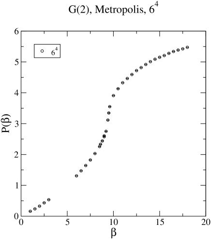
Figure 6: The plaquette expectation values as function of of $\beta$: $6^{4}$ lattice.

IV.2 Static Quark Potential

We are interested in demonstrating the “temporary confinement” property of G(2) gauge theory; i.e. the linearity of the static quark potential in some finite distance interval. The static quark potential can be calculated from Wilson loops of various sizes, but experience tells us that a “thin” Wilson line connecting the quark anti-quark sources has very little overlap with the ground state in quark anti-quark channel. Spatially smeared links (sometimes called “fat links”) are typically used for overlap enhancement. APE smearing Albanese:1987ds ; Teper:1987wt ; Perantonis:1988uz adds to particular link a weighted sum of its staples, but the subsequent projection onto a SU(N) element usually induces non-analyticities. Recently, the so-called “stout link” was introduced in Morningstar:2003gk ; in that approach the link variable remains in the SU(N) group during smearing.

All these methods produce time-consuming computer code when implemented for the G(2) gauge group. For this reason, we will use a variant of the smearing procedure outlined in Langfeld:2003ev , in which the spatial links for a given time-slice are cooled with respect to a D=3 dimensional lattice gauge action on the time slice. Consider a particular spatial link $U_{i}(x)$, $i=1\ldots 3$, and apply a trial update $U^{\prime}_{i}=G(\vec{\alpha})U_{i}$ where

$$G(\vec{\alpha})\;=\;\exp\Bigl{\{}\alpha_{a}C^{a}\Bigr{\}}\;,$$ (41)

and the $C^{a}$, $a=1\ldots 14$ are the generators of the G(2) algebra. If we denote by $M$ the sum of space-like plaquette variables containing the link $U_{i}(x)$ then the choice

$$\alpha_{a}\;=\;\epsilon\;\hbox{tr}\{C^{a}\,M\,\}\;,\hbox to28.45274pt{\hfill}\epsilon>0\;,$$ (42)

will always lead to an increase in $\hbox{tr}M$, for sufficiently small $\epsilon$, if the link $U_{i}(x)$ is replaced by the trial link. Our procedure is to start with $\epsilon\approx 1$, and replace links by trial links if $\hbox{tr}M$ is increased by the replacement. Proceeding through the lattice, $\epsilon$ is tuned so that at least 50% of the changes are accepted. One sweep through the lattice is one smearing step. As a stopping criterion, one might use the size of $\Delta S^{(3)}$ or a given number of smearing steps; our present present results were obtained with a fixed number of $70$ smearing steps.

Figure 7: $-\ln\langle W(r,t)\rangle$ as function of $n_{t}=t/a$ for several values of $n_{s}=r/a$ for a $12^{4}$ lattice and for $\beta=9.6$. The static potential as function of $r$ (right panel).

Let $W(r,t)$ denote the expectation value of a timelike, rectangular $r\times t$ Wilson loop, where $r=n_{s}a$ and $t=n_{t}a$, and $a$ is the lattice spacing. The sides of length $r,~{}t$ are oriented in spacelike and time directions, respectively. The spacelike links are taken to be the smeared links, while the timelike links are unmodified. For a fixed value of $r=an_{s}$, $V(r)$ is determined from a fit of $W(r,t)$, computed at various $n_{t}$, to the form

$$c\;+\;V(r)a\;n_{t}\;\approx\;-\ln\;\Bigl{\langle}W({\cal C})\Bigr{\rangle}\;.$$ (43)

Using smeared links, we find that $-\ln\;\langle W({\cal C})\rangle$ scales linearly with $n_{t}$ even for $n_{t}$ as small as $n_{t}=2$ (see figure 7 for an example at $\beta=9.6$). The corresponding linear fit yields $V(r)a$ including its error bar. Figure 7 (right panel) shows $V(r)a$ as function of $r/a$ again for $\beta=9.6$. The line between the static quarks (spacelike sides of the Wilson loops) runs parallel to one of the main axis (e.g. $(100)$) of the cubic lattice. In order to check for artifacts arising from the rotation symmetry breaking, the spacelike sides of the Wilson loop were also placed along the diagonal axis $(110)$ and $(111)$. From Figure 7 it is clear that at this coupling, the rotational symmetry breaking effects due to the underlying lattice structure are quite small.

The intermediate string tension $\sigma$ is extracted from a fit of the potential $V(r)$ to the form

$$V(r)\;=\;V_{0}\;+\;\sigma\,r\;-\;\frac{\alpha}{r}\;,$$ (44)

A sample fit at $\beta=9.6$ is shown in Fig. 7 (right panel). Results from $150$ independent lattice configurations have been have been taken into account. Fitting the data from Wilson loops placed along the main axis of the lattice ($(100)$-data), we find (with $n=r/a$)

$$V(r)a\;=\;0.713(7)\;-\;\frac{0.313(5)}{n}\;+\;0.141(2)\,n\;,\;\chi^{2}/\mathrm{dof}\approx 2.1\;.$$

Fitting data from all crystallographic orientations of the Wilson loops, we obtain

$$V(r)a\;=\;0.79(1)\;-\;\frac{0.34(1)}{n}\;+\;0.13(2)\,n\;,\;\chi^{2}/\mathrm{dof}\approx 9200\;.$$

The large value for $\chi^{2}/\mathrm{dof}$ in the latter case arises from the facts that (i) only statistically error bars are included in the data and that (ii) the error due to rotational symmetry breaking is much larger than the statistical one. Both fits are shown in figure 7 right panel.

Our numerical findings provide clear evidence of the linearity of the potential at intermediate distances $r$. At large distances $r$, one expects a flattening of the potential due to string breaking effects. From experience with SU(2) and SU(3) lattice theories, we do not expect to observe string breaking from measurements of modest-sized Wilson loops. String-breaking should be observable in sufficiently large Wilson loops, but this would require the rather more sophisticated noise reduction methods employed, e.g., in ref. dFK .

Figure 8: The static potential in units of the lattice spacing (left panel) and in units of the intermediate) string tension (right panel).

$\beta$	$9.5$	$9.6$	$9.7$	$9.8$	$9.9$	$10$
$\sigma a^{2}$	$0.24(2)$	$0.14(1)$	$0.102(3)$	$0.079(1)$	$0.060(2)$	$0.047(1)$
$\alpha$	$0.28(5)$	$0.313(2)$	$0.318(8)$	$0.311(2)$	$0.311(3)$	$0.309(4)$

Table 1: Lattice spacing $a$ in units of the string tension $\sigma$ for the values $\beta$; also shown $\alpha(\beta)$; $12^{4}$ lattice.

We have calculated the potential with $\beta$ in the range $[9.4,10]$ on a $12^{4}$ lattice volume. The “raw data” are shown in figure 8 (left panel). From a fit of the raw data to eq. (44), we have extracted the string tension in lattice units, $\sigma a^{2}$, at each $\beta$ value (see table 1). In order to avoid any obfuscation by rotational symmetry breaking effects, only data from Wilson loops with $(100)$-orientation have been included. The obtained values for the string tensions can be used to express the static potential in physical units, by first subtracting the self-energy $V_{0}(\beta)$ from the “raw” potential in lattice units, and dividing the result by $\sqrt{\sigma a^{2}}$. The result is plotted for several $\beta$ values as function of the distance in units of the physical string tension $\sqrt{\sigma}\,r=n_{s}\,\sqrt{\sigma a^{2}}$ (see figure 8, right panel). A fit of the data arising from all $\beta$-values to the potential $V(r)$ in (44) is also included to guide the eye. We observe that the data at different $\beta$ values lies on the same line, and that rotational symmetry breaking effects are small.

IV.3 Finite Temperature Transition

In SU(2) gauge-Higgs theory there is no unambiguous transition between the Higgs phase and the temporary confinement phase, and no local, gauge-invariant order parameter which can distinguish between the two phases (for a recent discussion, cf. ghiggs ). In particular, the center symmetry is trivial (i.e. $Z_{1}$), and Polyakov line VEVs are non-zero throughout the phase diagram. Nevertheless, there does exist a finite temperature transition in this theory, where the Polyakov line jumps from a small value to a larger value, and the linear potential at intermediate distances is lost.

Denote the Polyakov line as

$$P(\vec{x})\;=\;\prod_{t}U_{4}(t,\vec{x})\;.$$ (45)

The standard order parameter for finite temperature transitions is

$$p(T)\;=\;\left\langle\frac{1}{N^{3}}\left|\sum_{\vec{x}}\hbox{tr}\;P(\vec{x})\right|\right\rangle$$ (46)

on an $N^{3}\times N_{t}$ lattice, where the temperature is $T=1/(N_{t}\,a(\beta))$. It was observed in refs. Pepe1 ; Pepe2 that G(2) lattice gauge theory undergoes a first order transition at a finite temperature, indicated by a jump of $p(T)$ at $T_{c}$. As in SU(2) gauge-Higgs theory, this first-order transition cannot be characterized as a center symmetry-breaking transition.

Consider a gauge transformation of the Polyakov line holonomy

$$P^{\,\prime}(\vec{x})\;=\;\Omega(\vec{x},1)\,P(\vec{x})\,\Omega^{T}(\vec{x},1)\;,~{}~{}~{}~{}~{}~{}\Omega(\vec{x},1)\;=\;\Omega(\vec{x},N_{t})\;.$$ (47)

By a judicious choice of gauge transformation $\Omega=T\Omega$, where matrices $T$ and $\Omega$ are described in Appendix A and Appendix C, respectively, we may bring $P(x)$ into the form

$$T\;V\;P^{\,\prime}(\vec{x})\;V^{\dagger}\;T^{T}\;=\;\left(\begin{array}[]{ccc}1&0&0\\ 0&U_{ik}&0\\ 0&0&U^{\ast}_{lm}\end{array}\right)\;,~{}~{}~{}~{}U\;\in\;\mathrm{SU(3)}\;,$$ (48)

which emphasizes the SU(3) subgroup. The SU(3) subgroup is of interest here because the trace of a Polyakov line is the sum of its eigenvalues, the eigenvalues are elements of the Cartan subgroup, and the Cartan subgroup of G(2) is the same as that of the SU(3) subgroup. We have

$$\hbox{tr}\;P(\vec{x})\;=\;1\;+\;2\,\mbox{Re}\;\hbox{tr}U\;.$$ (49)

It is therefore sufficient to consider the trace of $3\times 3$ submatrix $U$. If the Polyakov line VEV were exactly zero (the case of true confinement, rather than temporary confinement), we would have

$$\Bigl{\langle}\frac{1}{3}\;\mbox{Re}\;\hbox{tr}U\Bigr{\rangle}\;=\;-\frac{1}{6}$$ (50)

exactly. However, because of color screening, this relation can only be approximately true at low temperatures.

Figure 9: Region of support for values $c(\vec{x})$ in (51) for $\beta=0$ (left panel). Right panel: Distribution of $c(\vec{x})$ at zero temperature (squares) and in the deconfinement phase (circles).

We define

$$c(\vec{x})=\frac{1}{3}\hbox{tr}U(\vec{x})$$ (51)

which takes values within the curved triangle shown in figure 9. The right panel of figure 9 shows the distribution of $c(\vec{x})$ for $\beta=9.7$ at low and high temperatures. At $\beta=9.7$ and a $6^{4}$ lattice (low temperature case), we clearly observe that the points accumulate near the non-trivial center elements of SU(3), i.e.,

$$c_{+}\;=\;-\,0.5\;+\;i\,\frac{\sqrt{3}}{2}\;,\hbox to28.45274pt{\hfill}c_{-}\;=\;-\,0.5\;-\;i\,\frac{\sqrt{3}}{2}\;.$$

As expected, the scatter plot is symmetric with respect to reflections across the $x$-axis. At temperatures $T>T_{c}$ ($6^{3}\times 2$ lattice volume), a strong shift of the data away from the non-trivial center elements towards the unit element is clearly observed.

V SU(3), $Z_{3}$, or SU(2) “Dominance”?

Although the center of the G(2) gauge group is trivial, one may ask if, in some gauge, the infrared dynamics is controlled by a subgroup of G(2) which does have a center. The motivation for this idea goes back to ’t Hooft’s proposal for abelian projection thooft-mon : In an SU(N) gauge theory, imagine imposing a gauge choice which leaves a remaining $U(1)^{N-1}$ gauge symmetry. The resulting theory can be thought of as a gauge theory with a compact abelian gauge group, whose degrees of freedom are “photons” and monopoles, coupled to a set of “matter” fields which consist of the gluons which are charged with respect to the $U(1)^{N-1}$ gauge group. If for some reason these gluons are very massive, then the idea is that they are irrelevant to the infrared physics, which is controlled by an effective abelian gauge theory. This is known as “abelian dominance”. Many numerical investigations have claimed to verify the existence of a large mass for the charged gluons. Confinement is then supposed to be due to the condensation of monopoles in the abelian theory.

In the same spirit, let us consider fixing the gauge of the G(2) theory, in such a way that the action remains invariant under an SU(3) subgroup of the G(2) gauge transformations. The gauge-fixed theory can be thought of as a theory of SU(3) gluons, coupled to vector matter fields (the remaining gluons of G(2)) and ghosts. If, for some unknown dynamical reason, these vector matter and ghost fields aquire a large effective mass, then the linear potential would be largely determined by pure SU(3) dynamics, and $Z_{3}$ vortices associated with the center of the SU(3) subgroup would be expected to carry the associated magnetic disorder.

To investigate this idea, we turn to lattice Monte Carlo simulations. We have found it useful, for the investigation of SU(3) dominance, to use the representation of the G(2) group by $7\times 7$ complex matrices, as presented in refs. Pepe2 ; Macfarlane . In this representation, any group element ${\large\cal G}\in G(2)$ can be expressed as

$${\large\cal G}={\cal Z}{\cal U}$$ (52)

where ${\cal Z}$ is a $7\times 7$ unitary matrix which is a function of a complex 3-vector $K$, and ${\cal U}$ is the matrix

$${\cal U}=\left(\begin{array}[]{ccc}U&&\cr&1&\cr&&U^{*}\end{array}\right)$$ (53)

where $U$ is a $3\times 3$ SU(3) matrix. The construction of the ${\large\cal Z}$ matrix from a complex 3-vector is described, following ref. Pepe2 , in Appendix D. The conjecture is that in a suitably chosen “maximal SU(3) gauge”, which brings the ${\large\cal Z}$ matrices in the ${\large\cal G}={\large\cal Z}{\large\cal U}$ link decomposition as close as possible, on average, to the unit matrix, the information about confinement in the intermediate distance regime is carried entirely by the ${\large\cal U}$ matrices. This means that the string tension of Wilson loops formed, in this gauge, from the $3\times 3$ $U$ matrices composing ${\large\cal U}$ would approximately reproduce the full intermediate-distance string tension, while the string tension of Wilson loops formed from the ${\large\cal Z}$ variables alone would vanish. If SU(3) dominance of this kind is exhibited by G(2) lattice gauge theory, then we can make a further reasonable conjecture, which is that the confinement information in the $U$ matrices is carried entirely by $Z_{3}$ center vortices. If so, then (i) the $Z_{3}$ vortices by themselves should also give a good estimate of the full intermediate string tension; and (ii) removing vortices from the ${\large\cal U}$ matrices should completely eliminate the intermediate string tension in G(2) loop holonomies.

We define maximal SU(3) gauge to be the gauge which minimizes

$$R_{1} = \sum_{x}\sum_{\mu=1}^{4}\left\{\sum_{i=1}^{3}\sum_{j=4}^{7}|u_{\mu}^{ij}(x)|^{2}+\sum_{i=5}^{7}\sum_{j=1}^{4}|u_{\mu}^{ij}(x)|^{2}\right.$$ (54)

$$\qquad+\left.\left(\sum_{j=1}^{3}+\sum_{j=5}^{7}\right)|u_{\mu}^{4j}(x)|^{2}\right\}$$

where $u_{\mu}^{ij}(x)$ is the $(i,j)$ component of the G(2) link variable (note that $R_{1}=0$ for ${\large\cal Z}=\mathbbm{1}_{7}$). It is straightforward to check that multiplying a link variable on either the left or the right by an SU(3) subgroup element ${\large\cal U}$ leaves $R_{1}$ unchanged; it is therefore sufficient to use only the $g={\large\cal Z}$ transformations in fixing the gauge. This also means that maximizing $R_{1}$ leaves a residual local SU(3) symmetry, so that “maximal SU(3) gauge” is a good name for this gauge choice. The next step is to use the remaining SU(3) gauge freedom to maximize

$$R_{2} = \sum_{x}\sum_{\mu=1}^{4}\left\{\Bigl{|}u_{\mu}^{11}(x)+u_{\mu}^{22}(x)+u_{\mu}^{33}(x)\Bigr{|}^{2}\right.$$ (55)

$$\qquad+\left.\Bigl{|}u_{\mu}^{55}(x)+u_{\mu}^{66}(x)+u_{\mu}^{77}(x)\Bigr{|}^{2}\right\}$$

leaving a remnant local $Z_{3}$ symmetry in “maximal $Z_{3}$ gauge.” This two-step process is reminiscent of fixing to indirect maximal center gauge in SU(N) gauge theory. Details regarding our Monte Carlo updating procedure in the complex representation of G(2), and the method of fixing to maximal SU(3) and maximal $Z_{3}$ gauges, can be found in Appendix D.

V.1 SU(3) and $\mathbf{Z_{3}}$ Projection

Having fixed to maximal $Z_{3}$ gauge, we compute the following observables:

1. Full Loops. Here we use the full G(2) link variables ${\large\cal G}={\large\cal Z}{\large\cal U}$ to compute Wilson loops, and of course gauge-fixing is irrelevant to the loop values.

2. SU(3) Projected Loops. These are loops computed from SU(3) link variables $U$, extracted from the top $3\times 3$ block of the $7\times 7$ ${\large\cal U}$ link matrices

   $${\cal U}=\left(\begin{array}[]{ccc}U&&\cr&1&\cr&&U^{*}\end{array}\right)$$ (56)

3. $\mathbf{Z_{3}}$ Projected Loops. These loops are just constructed from the $z_{\mu}(x)\in Z_{3}$ link variables obtained from center-projection of the $3\times 3$ $U$-link variables.

4. $\boldmath{\large\cal Z}$ Loops. These “SU(3)-suppressed” loops are computed from the ${\large\cal Z}$ link variables alone; i.e. we set the SU(3) part of the ${\large\cal G}={\large\cal Z}{\large\cal U}$ link variables to ${\large\cal U}=\mathbbm{1}_{7}$.

5. G(2) Vortex-Only Loops. In the decomposition of G(2) link variables ${\large\cal G}={\large\cal Z}{\large\cal U}$, replace the $SU(3)$ factor ${\large\cal U}$ by the vortex-only element

   $${\cal U}\rightarrow V\equiv\left(\begin{array}[]{ccc}zI_{3}&&\cr&1&\cr&&z^{*}I_{3}\end{array}\right)$$ (57)

   and compute loops with the $7\times 7$ link variables ${\large\cal G}={\large\cal Z}V$.

6. G(2) Vortex-Removed Loops. Here we remove vortices from the SU(3) elements ${\large\cal U}$ by the usual procedure dFE , and use the modified, vortex-removed ${\large\cal U}^{\prime}$, together with ${\large\cal Z}$, to construct vortex-removed G(2) lattice link variables ${\large\cal G}^{\prime}={\large\cal Z}{\large\cal U}^{\prime}$. In practice this accomplished simply by multiplying the original ${\large\cal G}$ by $V^{\dagger}$, i.e. construct loops from link variables

   $${\large\cal G}^{\prime}={\large\cal G}V^{\dagger}$$ (58)

7. SU(3) Vortex-Removed Loops. We construct loops from the SU(3)-projected, vortex-removed lattice $U^{\prime}=z^{*}U$.

Figure 10 shows our results for Creutz ratios of $Z_{3}$-projected configurations at couplings $\beta=9.5,~{}9.6,~{}9.7$. The straight lines shown are for the intermediate string tension at these couplings, extracted from the unprojected lattice and listed in Table 1 above. The agreement of the $Z_{3}$-projected string tension with the full intermediate string tension is quite good.

Figure 10: Creutz ratios for $Z_{3}$-projected loops at $\beta=9.5,9.6,9.7$. The horizontal lines show the values of the corresponding intermediate string tensions, computed in section IV on the unprojected lattice.

Figure 11: Creutz ratios for the full, $Z_{3}$-projected, G(2) vortex-only, and G(2) vortex-removed loops at $\beta=9.7$

Figure 11 shows the data, at $\beta=9.7$ on a $10^{4}$ lattice, for Creutz ratios obtained from full, G(2) vortex-only, G(2) vortex-removed, and $Z_{3}$ projected configurations. Again, denoting the decomposition of the full links in maximal $Z_{3}$ gauge by ${\large\cal G}={\large\cal Z}{\large\cal U}$, and the Z(3)-projection of ${\large\cal U}$ (eq. 57) by $V$, then the G(2) vortex-only link variables are ${\large\cal G}_{vo}={\large\cal Z}V$, and the G(2) vortex-removed links are ${\large\cal G}_{vrem}={\large\cal Z}{\large\cal U}V^{\dagger}$. It is clear from the plot that the G(2) vortex-only data appoaches the data obtained from full Wilson loops, while the linear potential is absent in the vortex-removed data.

If the confining disorder resides in the $Z_{3}$ degrees of freedom, and these in turn lie in the SU(3) projected link variables, then SU(3) Dominance is implied. The string tension on the unprojected lattice should be seen in the SU(3) projection, and removing SU(3) fluctuations from the G(2) link variables should send the intermediate string tension to zero. Both of these phenomena can be seen in Fig. 12. The suppression of the full string tension in the ${\large\cal Z}$ loops, which follows from suppression of SU(3) fluctuations, is particularly striking.

Finally, we can remove vortices from the SU(3) link variables, and compute Creutz ratios from those lattices. The results for $\beta=9.6$ and $\beta=9.7$ are displayed in Fig. 13, and appear to be consistent with a vanishing string tension for large loops.

Figure 12: Creutz ratios for SU(3) projected lattices, and for G(2) lattices with the SU(3) link factors set to unity (“SU(3) suppressed”).

Figure 13: Creutz ratios for SU(3)-projected, vortex-removed Wilson loops, at $\beta=9.6,~{}9.7$.

V.2 Problems with the Projections

The success of SU(3) and $Z_{3}$-projected lattices in reproducing the asymptotic string tension of G(2) gauge theory, together with the vanishing string tension in “vortex-removed” lattices, tends to obscure the fact that these are, after all, gauge-dependent observables. That fact doesn’t necessarily mean that, e.g., the $Z_{3}$ vortices located via projection are unphysical, but neither do the projected results alone prove that these are physical objects. The really crucial numerical evidence in favor of the physical nature of vortices, in SU(2) and SU(3) gauge theories, was the correlations that were found found between P-vortex location and gauge-invariant observables. In particular

1. Plaquettes at the location of P-vortices have, on the unprojected lattice, a plaquette action which is significantly higher than average.

2. A vortex-limited Wilson loop $W_{n}(C)$ is an unprojected Wilson loop, evaluated in an ensemble of configurations in which $n$ P-vortices pierce the loop of the projected lattice. It has been found that as the loop area becomes large

   $$\frac{W_{n}(C)}{W_{0}(C)}\rightarrow e^{2\pi in/N}$$ (59)

   where $N$ is the number of colors. This is the expected behavior, if a P-vortex on the projected lattice locates a thick vortex on the unprojected lattice.

3. In an SU(N) gauge theory, a Wilson loop calculated in the “vortex-removed” lattice can be equally well described as the expectation value of the product

   $$W_{vrem}(C)=\langle Z^{*}(C)\hbox{Tr}[U(C)]\rangle$$ (60)

   where $Z(C),~{}U(C)$ are loop holonomies on the projected and unprojected lattices, respectively. If $W_{vrem}$ has a vanishing asymptotic string tension, then this fact translates directly into a correlation of the phase of the projected loop $Z(C)$, induced by P-vortices, with the phase of the gauge-invariant observable $\hbox{Tr}[U(C)]$ on the unprojected lattice.

Unlike the SU(2) and SU(3) cases, we have so far found no discernable correlation between gauge-invariant G(2) Wilson loops, and the SU(3) and $Z_{3}$ projected loops. Plaquettes pierced by $Z_{3}$ vortices have no higher action, on the unprojected lattice, than other plaquettes, and the VEVs of vortex-limited Wilson loops $W_{n}(C)$ appear to be completely independent of the number of vortices $n$. Although the string tension of vortex-removed loops vanishes in G(2) gauge theory, the vortex-removed loops $W_{vrem}(C)$ cannot be expressed as a product of vortex loops and gauge-invariant loops, hence the VEV of $W_{vrem}(C)$ does not directly correlate the vortex observables with gauge-invariant observables. It should be noted that in SU(N) gauge theories, vortex removal is a very minimal disturbance of the lattice, especially at weak couplings. Vortex removal affects the plaquette action only at the location of P-plaquettes, whose density falls exponentially with coupling $\beta$. In G(2) gauge theory, matters are different. In that case $Z_{3}$ vortex removal is a serious butchery of the original configuration, affecting every plaquette of the lattice.

For these reasons, we think that the results of SU(3) and $Z_{3}$ projection in G(2) gauge theory are misleading. In particular, the supposed vortices located by $Z_{3}$ projection appear to not affect any local gauge-invariant observables (i.e. Wilson loops), and on these grounds we believe that the objects identified by $Z_{3}$ projection are simply unphysical. For these reasons, we think that the results of SU(3) and $Z_{3}$ projection in G(2) gauge theory are misleading. In particular, the supposed vortices located by $Z_{3}$ projection appear to not affect any local gauge-invariant observables (i.e. Wilson loops), and on these grounds we believe that the objects identified by $Z_{3}$ projection are simply unphysical.

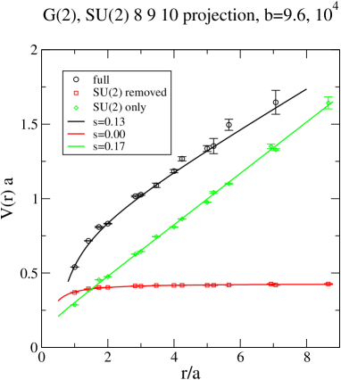
Figure 14: The G(2) static potential, compared to the static potentials computed in SU(2)-only and SU(2)-removed lattices, at $\beta=9.6$. String tensions $s=\sigma a^{2}$ are extracted from fits to eq. (44).

One might ask if the reason for the ultimate failure of the SU(3) and $Z_{3}$ projections lies in the choice of the subgroup. If we would calculate Wilson loops from the $7\times 7$ SU(3)-projected link variables ${\large\cal U}$, rather than the $3\times 3$ SU(3) link variables $U$, then those Wilson loops would not have an area law, due to the unit element in the $7\times 7$ ${\large\cal U}$ matrix; i.e. the existence of an element of the fundamental representation of G(2) which transforms as a singlet under the SU(3) subgroup. Suppose that we instead look for the smallest subgroup of G(2) such that all elements of the fundamental representation of G(2) transform as non-singlets under that subgroup. It turns out that the SU(2) subgroup defined by the generators $C_{8},C_{9},C_{10}$ (see Appendix A) satisfies this condition; the fundamental representation of G(2) transforms, under this subgroup, as a triplet and two doublets.

We then impose a “maximal SU(2)” gauge, and calculate the Wilson loops of the SU(2)-only and SU(2)-removed link variables. The results are impressive, and are displayed in Fig. 14. However, up to now we have not found any significant correlation between SU(2)-only and G(2) Wilson loops, and in this respect the SU(2) projection appears to be also problematic.

We believe that the reason that SU(3), $Z_{3}$, and SU(2)-projected loops apparently fail to correlate with gauge-invariant observables is that these projections have no gauge-invariant motivation from the beginning. We may reasonably suppose that a gauge theory with gauge group $G$ is “dominated” by the degrees of freedom associated with a subgroup $H$, if, independent of any gauge-fixing, the gauge-invariant string tension depends only on the representation of the subgroup. This is the case for the $Z_{N}$ center subgroup of SU(N) gauge theories, at large distance scales. Center projection is then a method for isolating the large-scale confining fluctuations. In contrast, the SU(3), $Z_{3}$, and SU(2) subgroups of G(2) have no relation to G(2) Casimir scaling, at intermediate distances, nor are any of these subgroups singled out at large scales, where the string tension vanishes for any representation. In fact, similar remarks can be made regarding abelian projection in pure SU(N) gauge theories, which we used to motivate the subgroup projections of this section. The abelian U(1)^N-1 subgroup cannot easily account for Casimir scaling at intermediate distances, while at asymptotic distances the string tension of an abelian-projected loop in fact depends only on the N-ality, rather than the abelian charge of the loop j3 .

VI Conclusions

In this article we have presented a unified picture of vacuum fluctuations in G(2) and SU(N) gauge theories, in which a two-dimensional surface slice of the four-dimensional lattice can be decomposed into domains corresponding to elements of the gauge group center. Domains associated with center elements different from the identity are just two-dimensional cross-sections of the usual $Z_{N}$ vortices; the new feature is that we also allow for domains associated with the unit center element, which exists in G(2) as well as SU(N). This domain structure accounts for the representation dependence of the asymptotic string tension on the center subgroup, which in the case of G(2) implies a vanishing asymptotic string tension. The existence and Casimir scaling of the linear potential at intermediate distances is explained by random spatial variations of the color magnetic flux in the interior of the center domains.

The picture we have outlined is a kind of phenomenology. Domain structure is arrived at by simply asking what features of typical vacuum fluctuations, in a Euclidean 4-volume, can account for both Casimir scaling of intermediate string tensions, and color-screening in the asymptotic string tensions. Of course one would like to support this picture by either analytical methods or numerical simulations. There is, in fact, abundant numerical evidence for the relevance of $Z_{2}$ and $Z_{3}$ center vortices in SU(2) and SU(3) lattice gauge theories review ; michael , but unfortunately the usual tools which are used to locate such vortices in lattice simulations (i.e. center projection in maximal center gauge) are not of much use in locating domains associated with the unit element. At the moment we can only appeal to a number of analytical studies of the one-loop effective action of vortex configurations, which show that this action is stationary for magnetic flux quantized in units corresponding to the gauge group center elements, including the unit element Hugo ; Diakonov ; Bordag . Thus the dynamics underlying center vortex formation may ultimately be the same for the unit and non-unit element varieties. The picture we have presented for Casimir scaling at intermediate distance scales is motivated by the notion of dimensional reduction, and by various approximate treatments of the Yang-Mills vacuum wavefunctional Me1 ; Me2 ; Mansfield ; Nair ; Leigh ; Freidel .

We have also calculated certain static properties of G(2) lattice gauge theory, namely, the intermediate string tension, and the distribution of Polyakov line holonomies at zero and finite temperature. We see very clear evidence of a linear potential in the fundamental representation, but we have not attempted to compute the potential for higher representations, needed to verify Casimir scaling, or the operator-mixings needed to see string breaking. These are left for future investigations. The eigenvalues of the Polyakov line are those of the SU(3) subgroup, and we have shown that the finite temperature phase transition is accompanied by a shift in the concentration of the Polyakov line eigenvalues from non-trivial to trivial SU(3) center elements.

Finally, we have investigated projection of G(2) link variables to various subgroups. These projections, to SU(3), $Z_{3}$, and SU(2) subgroups, so far lack the gauge-invariant motivation that exists for center projection in SU(N) gauge theories, where the representation dependence of the asymptotic string tension is given entirely by the representation of the $Z_{N}$ subgroup. The SU(3), $Z_{3}$, and SU(2) subgroups of G(2) have no natural connection to either G(2) Casimir scaling at intermediate distances, where a non-zero string tension exists, or to the asymptotic regime, where the string tension vanishes. The fact that we have found no correlation whatever, between the projected Wilson loops and gauge-invariant observables in G(2) gauge theory, probably reflects the fact that these subgroups do not appear naturally in any gauge-invariant set of observables. The only subgroup which really does appear to be relevant to pure non-abelian gauge theories is the center subgroup, and this relevance persists even in cases such as G(2) gauge theory, where the center subgroup consists of only a single unit element.

Appendix A G(2) algebra

In the following, we will study the fundamental representation of G(2) in more detail. In this representation, the generators can be chosen as real $7\times 7$ matrices. The group elements $U$ satisfy the constraints

$$U\,U^{T}\;=\;1\;,\hbox to28.45274pt{\hfill}T_{abc}\;=\;T_{def}\;U_{da}\;U_{eb}\;U_{fc}\;,$$ (61)

where $T_{abc}$ is a total anti-symmetric tensor Pepe1 . The group elements are generated by the Lie algebra:

$$U\;=\;\exp\left\{-i\,\sum_{a=1}^{14}\rho_{a}\;iC_{a}\right\}\;,\hbox to28.45274pt{\hfill}\rho\in{\cal R}^{14}\;.$$ (62)

An explicit realization of the generators $i\,C_{a}$ was presented in Cacciatori:2005yb . For the readers convenience, these matrices are provided below. For this choice of representation, these elements are

$$T_{123}\;=\;T_{145}\;=\;T_{176}\;=\;T_{246}\;=\;T_{257}\;=\;T_{347}\;=\;T_{365}\;=\;1\;.$$ (63)

All linear combinations of the generators $C_{a}$ form the vector space $L$ of the Lie algebra.

The embedding of $G(2)$ in the group $SO(7)$ is generated by the $14$ Lie algebra elements $C_{k},k=1,\ldots,14$:

$$C_{1} = \left(\begin{array}[]{ccccccc}0&0&0&0&0&0&0\\ 0&0&0&0&0&0&0\\ 0&0&0&0&0&0&0\\ 0&0&0&0&0&0&-1\\ 0&0&0&0&0&-1&0\\ 0&0&0&0&1&0&0\\ 0&0&0&1&0&0&0\end{array}\right)\qquad C_{2}=\left(\begin{array}[]{ccccccc}0&0&0&0&0&0&0\\ 0&0&0&0&0&0&0\\ 0&0&0&0&0&0&0\\ 0&0&0&0&0&1&0\\ 0&0&0&0&0&0&-1\\ 0&0&0&-1&0&0&0\\ 0&0&0&0&1&0&0\end{array}\right)$$ (78)

$$C_{3} = \left(\begin{array}[]{ccccccc}0&0&0&0&0&0&0\\ 0&0&0&0&0&0&0\\ 0&0&0&0&0&0&0\\ 0&0&0&0&-1&0&0\\ 0&0&0&1&0&0&0\\ 0&0&0&0&0&0&-1\\ 0&0&0&0&0&1&0\end{array}\right)\qquad C_{4}=\left(\begin{array}[]{ccccccc}0&0&0&0&0&0&0\\ 0&0&0&0&0&0&1\\ 0&0&0&0&0&1&0\\ 0&0&0&0&0&0&0\\ 0&0&0&0&0&0&0\\ 0&0&-1&0&0&0&0\\ 0&-1&0&0&0&0&0\end{array}\right)$$ (93)

$$C_{5} = \left(\begin{array}[]{ccccccc}0&0&0&0&0&0&0\\ 0&0&0&0&0&-1&0\\ 0&0&0&0&0&0&1\\ 0&0&0&0&0&0&0\\ 0&0&0&0&0&0&0\\ 0&1&0&0&0&0&0\\ 0&0&-1&0&0&0&0\end{array}\right)\qquad C_{6}=\left(\begin{array}[]{ccccccc}0&0&0&0&0&0&0\\ 0&0&0&0&1&0&0\\ 0&0&0&-1&0&0&0\\ 0&0&1&0&0&0&0\\ 0&-1&0&0&0&0&0\\ 0&0&0&0&0&0&0\\ 0&0&0&0&0&0&0\end{array}\right)$$ (108)

$$C_{7} = \left(\begin{array}[]{ccccccc}0&0&0&0&0&0&0\\ 0&0&0&-1&0&0&0\\ 0&0&0&0&-1&0&0\\ 0&1&0&0&0&0&0\\ 0&0&1&0&0&0&0\\ 0&0&0&0&0&0&0\\ 0&0&0&0&0&0&0\end{array}\right)\qquad C_{8}=\frac{1}{\sqrt{3}}\left(\begin{array}[]{ccccccc}0&0&0&0&0&0&0\\ 0&0&-2&0&0&0&0\\ 0&2&0&0&0&0&0\\ 0&0&0&0&1&0&0\\ 0&0&0&-1&0&0&0\\ 0&0&0&0&0&0&-1\\ 0&0&0&0&0&1&0\end{array}\right)$$ (123)

$$C_{9} = \frac{1}{\sqrt{3}}\left(\begin{array}[]{ccccccc}0&-2&0&0&0&0&0\\ 2&0&0&0&0&0&0\\ 0&0&0&0&0&0&0\\ 0&0&0&0&0&0&1\\ 0&0&0&0&0&-1&0\\ 0&0&0&0&1&0&0\\ 0&0&0&-1&0&0&0\end{array}\right)\qquad C_{10}=\frac{1}{\sqrt{3}}\left(\begin{array}[]{ccccccc}0&0&-2&0&0&0&0\\ 0&0&0&0&0&0&0\\ 2&0&0&0&0&0&0\\ 0&0&0&0&0&-1&0\\ 0&0&0&0&0&0&-1\\ 0&0&0&1&0&0&0\\ 0&0&0&0&1&0&0\end{array}\right)$$ (138)

$$C_{11} = \frac{1}{\sqrt{3}}\left(\begin{array}[]{ccccccc}0&0&0&-2&0&0&0\\ 0&0&0&0&0&0&-1\\ 0&0&0&0&0&1&0\\ 2&0&0&0&0&0&0\\ 0&0&0&0&0&0&0\\ 0&0&-1&0&0&0&0\\ 0&1&0&0&0&0&0\end{array}\right)\qquad C_{12}=\frac{1}{\sqrt{3}}\left(\begin{array}[]{ccccccc}0&0&0&0&-2&0&0\\ 0&0&0&0&0&1&0\\ 0&0&0&0&0&0&1\\ 0&0&0&0&0&0&0\\ 2&0&0&0&0&0&0\\ 0&-1&0&0&0&0&0\\ 0&0&-1&0&0&0&0\end{array}\right)$$ (153)

$$C_{13} = \frac{1}{\sqrt{3}}\left(\begin{array}[]{ccccccc}0&0&0&0&0&-2&0\\ 0&0&0&0&-1&0&0\\ 0&0&0&-1&0&0&0\\ 0&0&1&0&0&0&0\\ 0&1&0&0&0&0&0\\ 2&0&0&0&0&0&0\\ 0&0&0&0&0&0&0\end{array}\right)\qquad C_{14}=\frac{1}{\sqrt{3}}\left(\begin{array}[]{ccccccc}0&0&0&0&0&0&-2\\ 0&0&0&1&0&0&0\\ 0&0&0&0&-1&0&0\\ 0&-1&0&0&0&0&0\\ 0&0&1&0&0&0&0\\ 0&0&0&0&0&0&0\\ 2&0&0&0&0&0&0\end{array}\right)$$ (168)

The two matrices $C_{3}$ and $C_{8}$ generate the Cartan subgroup of $G(2)$. Furthermore, there are 6 $SU(2)$ subgroups generated by the elements:

$$\begin{array}[]{llll}C_{1},&C_{2},&Y_{1}:=C_{3},&[C_{1},C_{2}]=2Y_{1},\\ C_{4},&C_{5},&Y_{2}:=\frac{1}{2}\left(\sqrt{3}C_{8}+C_{3}\right),&[C_{4},C_{5}]=2Y_{2}\\ C_{6},&C_{7},&Y_{3}:=\frac{1}{2}\left(-\sqrt{3}C_{8}+C_{3}\right),&[C_{6},C_{7}]=2Y_{3}\\ \sqrt{3}C_{9},&\sqrt{3}C_{10},&Y_{4}:=\sqrt{3}C_{8},&[\sqrt{3}C_{9},\sqrt{3}C_{10}]=2Y_{4}\\ \sqrt{3}C_{11},&\sqrt{3}C_{12},&Y_{5}:=\frac{1}{2}\left(-\sqrt{3}C_{8}+3C_{3}\right),&[\sqrt{3}C_{11},\sqrt{3}C_{12}]=2Y_{5}\\ \sqrt{3}C_{13},&\sqrt{3}C_{14},&Y_{6}:=\frac{1}{2}\left(\sqrt{3}C_{8}+3C_{3}\right),&[\sqrt{3}C_{13},\sqrt{3}C_{14}]=2Y_{6}\end{array}\,.$$ (175)

The first three $SU(2)$ subgroups form $4$ dimensional real representations of $SU(2)$ as subgroups of $SO(7)$ and they generate an $SU(3)$ subgroup of $G(2)$. The representations of the remaining three $SU(2)$ subgroups (as subgroups of $SO(7)$) are a little bit more complicated - they are $7$ dimensional but they are reducible: the representation space is the direct sum of a $3$ dimensional adjoint representation and a $4$ dimensional real representation (as in the case of the first three $SU(2)$ subgroups).

The various $SU(2)$ subgroups of $G(2)\subset SO(7)$ are obtained by exponentiation:

$$\exp(\alpha_{1}C_{1}+\alpha_{2}C_{2}+\alpha_{3}Y_{1})$$ (190)

$$= \left(\begin{array}[]{ccccccc}1&0&0&0&0&0&0\\ 0&1&0&0&0&0&0\\ 0&0&1&0&0&0&0\\ 0&0&0&\cos\alpha&-\hat{\alpha}_{3}\sin\alpha&\hat{\alpha}_{2}\sin\alpha&-\hat{\alpha}_{1}\sin\alpha\\ 0&0&0&\hat{\alpha}_{3}\sin\alpha&\cos\alpha&-\hat{\alpha}_{1}\sin\alpha&-\hat{\alpha}_{2}\sin\alpha\\ 0&0&0&-\hat{\alpha}_{2}\sin\alpha&\hat{\alpha}_{1}\sin\alpha&\cos\alpha&-\hat{\alpha}_{3}\sin\alpha\\ 0&0&0&\hat{\alpha}_{1}\sin\alpha&\hat{\alpha}_{2}\sin\alpha&\hat{\alpha}_{3}\sin\alpha&\cos\alpha\end{array}\right)=\left(\begin{array}[]{ccccccc}1&0&0&0&0&0&0\\ 0&1&0&0&0&0&0\\ 0&0&1&0&0&0&0\\ 0&0&0&a_{0}&-a_{3}&a_{2}&-a_{1}\\ 0&0&0&a_{3}&a_{0}&-a_{1}&-a_{2}\\ 0&0&0&-a_{2}&a_{1}&a_{0}&-a_{3}\\ 0&0&0&a_{1}&a_{2}&a_{3}&a_{0}\end{array}\right)$$

$$\exp(\alpha_{1}C_{4}+\alpha_{2}C_{5}+\alpha_{3}Y_{2})$$ (205)

$$= \left(\begin{array}[]{ccccccc}1&0&0&0&0&0&0\\ 0&\cos\alpha&-\hat{\alpha}_{3}\sin\alpha&0&0&-\hat{\alpha}_{2}\sin\alpha&\hat{\alpha}_{1}\sin\alpha\\ 0&\hat{\alpha}_{3}\sin\alpha&\cos\alpha&0&0&\hat{\alpha}_{1}\sin\alpha&\hat{\alpha}_{2}\sin\alpha\\ 0&0&0&1&0&0&0\\ 0&0&0&0&1&0&0\\ 0&\hat{\alpha}_{2}\sin\alpha&-\hat{\alpha}_{1}\sin\alpha&0&0&\cos\alpha&-\hat{\alpha}_{3}\sin\alpha\\ 0&-\hat{\alpha}_{1}\sin\alpha&-\hat{\alpha}_{2}\sin\alpha&0&0&\hat{\alpha}_{3}\sin\alpha&\cos\alpha\end{array}\right)=\left(\begin{array}[]{ccccccc}1&0&0&0&0&0&0\\ 0&a_{0}&-a_{3}&0&0&-a_{2}&a_{1}\\ 0&a_{3}&a_{0}&0&0&a_{1}&a_{2}\\ 0&0&0&1&0&0&0\\ 0&0&0&0&1&0&0\\ 0&a_{2}&-a_{1}&0&0&a_{0}&-a_{3}\\ 0&-a_{1}&-a_{2}&0&0&a_{3}&a_{0}\\ \end{array}\right)$$

$$\exp(\alpha_{1}C_{6}+\alpha_{2}C_{7}+\alpha_{3}Y_{3})=$$ (220)

$$= \left(\begin{array}[]{ccccccc}1&0&0&0&0&0&0\\ 0&\cos\alpha&\hat{\alpha}_{3}\sin\alpha&-\hat{\alpha}_{2}\sin\alpha&\hat{\alpha}_{1}\sin\alpha&0&0\\ 0&-\hat{\alpha}_{3}\sin\alpha&\cos\alpha&-\hat{\alpha}_{1}\sin\alpha&-\hat{\alpha}_{2}\sin\alpha&0&0\\ 0&\hat{\alpha}_{2}\sin\alpha&\hat{\alpha}_{1}\sin\alpha&\cos\alpha&-\hat{\alpha}_{3}\sin\alpha&0&0\\ 0&-\hat{\alpha}_{1}\sin\alpha&\hat{\alpha}_{2}\sin\alpha&\hat{\alpha}_{3}\sin\alpha&\cos\alpha&0&0\\ 0&0&0&0&0&1&0\\ 0&0&0&0&0&0&1\\ \end{array}\right)=\left(\begin{array}[]{ccccccc}1&0&0&0&0&0&0\\ 0&a_{0}&a_{3}&-a_{2}&a_{1}&0&0\\ 0&-a_{3}&a_{0}&-a_{1}&-a_{2}&0&0\\ 0&a_{2}&a_{1}&a_{0}&-a_{3}&0&0\\ 0&-a_{1}&a_{2}&a_{3}&a_{0}&0&0\\ 0&0&0&0&0&1&0\\ 0&0&0&0&0&0&1\\ \end{array}\right)$$

$$\exp(\alpha_{1}\sqrt{3}C_{9}+\alpha_{2}\sqrt{3}C_{10}+\alpha_{3}Y_{4})$$ (223)

$$= \left(\begin{array}[]{cc}A&0\\ 0&B\end{array}\right)$$

where

$$\alpha=\sqrt{\alpha_{1}^{2}+\alpha_{2}^{2}+\alpha_{3}^{2}}~{}~{}~{},~{}~{}~{}\hat{\alpha}_{k}=\frac{\alpha_{k}}{\alpha}~{}~{}~{},~{}~{}~{}a_{0}=\cos\alpha~{}~{}~{},~{}~{}~{}a_{k}=\hat{\alpha}_{k}\sin\alpha$$ (224)

and

$$A = \left(\begin{array}[]{ccc}2\cos^{2}\alpha-1+2\hat{\alpha}_{3}\hat{\alpha}_{3}\sin^{2}\alpha&-\hat{\alpha}_{1}\sin 2\alpha-\hat{\alpha}_{2}\hat{\alpha}_{3}\sin^{2}\alpha&-\hat{\alpha}_{2}\sin 2\alpha+\hat{\alpha}_{1}\hat{\alpha}_{3}\sin^{2}\alpha\\ \hat{\alpha}_{1}\sin 2\alpha-\hat{\alpha}_{2}\hat{\alpha}_{3}\sin^{2}\alpha&2\cos^{2}\alpha-1+2\hat{\alpha}_{2}\hat{\alpha}_{2}\sin^{2}\alpha&-\hat{\alpha}_{3}\sin 2\alpha-\hat{\alpha}_{1}\hat{\alpha}_{2}\sin^{2}\alpha\\ \hat{\alpha}_{2}\sin 2\alpha+\hat{\alpha}_{1}\hat{\alpha}_{3}\sin^{2}\alpha&\hat{\alpha}_{3}\sin 2\alpha-\hat{\alpha}_{1}\hat{\alpha}_{2}\sin^{2}\alpha&2\cos^{2}\alpha-1+2\hat{\alpha}_{1}\hat{\alpha}_{1}\sin^{2}\alpha\end{array}\right)$$ (228)

$$B = \left(\begin{array}[]{cccc}\cos\alpha&\hat{\alpha}_{3}\sin\alpha&-\hat{\alpha}_{2}\sin\alpha&\hat{\alpha}_{1}\sin\alpha\\ -\hat{\alpha}_{3}\sin\alpha&\cos\alpha&-\hat{\alpha}_{1}\sin\alpha&-\hat{\alpha}_{2}\sin\alpha\\ \hat{\alpha}_{2}\sin\alpha&\hat{\alpha}_{1}\sin\alpha&\cos\alpha&-\hat{\alpha}_{3}\sin\alpha\\ -\hat{\alpha}_{1}\sin\alpha&\hat{\alpha}_{2}\sin\alpha&\hat{\alpha}_{3}\sin\alpha&\cos\alpha\end{array}\right)$$ (233)

The elements of the two remaining $SU(2)$ subgroups look quite similar.

Alternatively, one may equally well use a complex representation of $G(2)$, as in refs. Pepe1 ; Pepe2 and in section V of this article. The two representations can be related by a similarity transformation $\tilde{C}_{k}=VC_{k}V^{\dagger}$, where $V$ is the unitary matrix

$$V = \frac{1}{\sqrt{2}}\left(\begin{array}[]{ccccccc}\sqrt{2}&0&0&0&0&0&0\\ 0&-i&-1&0&0&0&0\\ 0&-1&-i&0&0&0&0\\ 0&0&0&i&1&0&0\\ 0&0&0&1&i&0&0\\ 0&0&0&0&0&i&-1\\ 0&0&0&0&0&1&-i\end{array}\right)=\frac{1}{\sqrt{2}}\left(\begin{array}[]{cccc}\sqrt{2}&0&0&0\\ 0&-i\mathbbm{1}-\sigma_{1}&0&0\\ 0&0&i\mathbbm{1}+\sigma_{1}&0\\ 0&0&0&i\sigma_{3}-i\sigma_{2}\\ \end{array}\right)$$ (245)

and in particular

$$\tilde{C}_{1} = \left(\begin{array}[]{cccc}0&0&0&0\\ 0&0&0&0\\ 0&0&0&i\sigma_{3}\\ 0&0&i\sigma_{3}&0\\ \end{array}\right)\,,\,\tilde{C}_{2}=\left(\begin{array}[]{cccc}0&0&0&0\\ 0&0&0&0\\ 0&0&0&\mathbbm{1}\\ 0&0&-\mathbbm{1}&0\\ \end{array}\right)\,,\,\tilde{C}_{3}=\left(\begin{array}[]{cccc}0&0&0&0\\ 0&0&0&0\\ 0&0&-i\sigma_{3}&0\\ 0&0&0&i\sigma_{3}\\ \end{array}\right)\,,\,$$ (258)

$$\tilde{C}_{4} = \left(\begin{array}[]{cccc}0&0&0&0\\ 0&0&0&i\sigma_{3}\\ 0&0&0&0\\ 0&i\sigma_{3}&0&0\\ \end{array}\right)\,,\,\tilde{C}_{5}=\left(\begin{array}[]{cccc}0&0&0&0\\ 0&0&0&\mathbbm{1}\\ 0&0&0&0\\ 0&-\mathbbm{1}&0&0\\ \end{array}\right)\,,\,\tilde{C}_{6}=\left(\begin{array}[]{cccc}0&0&0&0\\ 0&0&i\sigma_{3}&0\\ 0&i\sigma_{3}&0&0\\ 0&0&0&0\\ \end{array}\right)\,,\,$$ (271)

$$\tilde{C}_{7} = \left(\begin{array}[]{cccc}0&0&0&0\\ 0&0&-\mathbbm{1}&0\\ 0&\mathbbm{1}&0&0\\ 0&0&0&0\\ \end{array}\right)\,,\,\tilde{C}_{8}=\frac{1}{\sqrt{3}}\left(\begin{array}[]{cccc}0&0&0&0\\ 0&-2i\sigma_{3}&0&0\\ 0&0&i\sigma_{3}&0\\ 0&0&0&i\sigma_{3}\\ \end{array}\right)$$ (280)

Finally one can use the (unitary) permutation matrix

$$T = \left(\begin{array}[]{ccccccc}1&0&0&0&0&0&0\\ 0&0&0&0&0&0&1\\ 0&0&0&0&1&0&0\\ 0&0&1&0&0&0&0\\ 0&0&0&0&0&1&0\\ 0&0&0&1&0&0&0\\ 0&1&0&0&0&0&0\end{array}\right)$$ (288)

to rearrange the rows and columns of $\tilde{C}_{1},\ldots,\tilde{C}_{8}$ such that it is obvious that the decomposition of the $7$-dimensional $SU(3)$ representation is given by $\{1\}\oplus\{3\}\oplus\{\bar{3}\}$.

Appendix B Euler decomposition of G(2)

In order to implement a Metropolis update, we will use prototypes of $G(2)$ group elements to maneuver through group space. These are:

$$D_{1}(\alpha) = \exp\left\{\alpha C_{1}\right\}\;=\;\left(\begin{array}[]{ccccccc}1&0&0&0&0&0&0\\ 0&1&0&0&0&0&0\\ 0&0&1&0&0&0&0\\ 0&0&0&\hbox{ $\cos\alpha$}&0&0&-\hbox{ $\sin\alpha$}\\ 0&0&0&0&\hbox{ $\cos\alpha$}&-\hbox{ $\sin\alpha$}&0\\ 0&0&0&0&\hbox{ $\sin\alpha$}&\hbox{ $\cos\alpha$}&0\\ 0&0&0&\hbox{ $\sin\alpha$}&0&0&\hbox{ $\cos\alpha$}\end{array}\right),$$ (296)

$$D_{2}(\alpha) = \exp\left\{\alpha C_{2}\right\}\;=\;\left(\begin{array}[]{ccccccc}1&0&0&0&0&0&0\\ 0&1&0&0&0&0&0\\ 0&0&1&0&0&0&0\\ 0&0&0&\hbox{ $\cos\alpha$}&0&\hbox{ $\sin\alpha$}&0\\ 0&0&0&0&\hbox{ $\cos\alpha$}&0&-\hbox{ $\sin\alpha$}\\ 0&0&0&-\hbox{ $\sin\alpha$}&0&\hbox{ $\cos\alpha$}&0\\ 0&0&0&0&\hbox{ $\sin\alpha$}&0&\hbox{ $\cos\alpha$}\end{array}\right),$$ (304)

$$D_{3}(\alpha) = \exp\left\{\alpha C_{3}\right\}\;=\;\left(\begin{array}[]{ccccccc}1&0&0&0&0&0&0\\ 0&1&0&0&0&0&0\\ 0&0&1&0&0&0&0\\ 0&0&0&\hbox{ $\cos\alpha$}&-\hbox{ $\sin\alpha$}&0&0\\ 0&0&0&\hbox{ $\sin\alpha$}&\hbox{ $\cos\alpha$}&0&0\\ 0&0&0&0&0&\hbox{ $\cos\alpha$}&-\hbox{ $\sin\alpha$}\\ 0&0&0&0&0&\hbox{ $\sin\alpha$}&\hbox{ $\cos\alpha$}\end{array}\right),$$ (312)

$$D_{4}(\alpha) = \exp\left\{\alpha C_{4}\right\}\;=\;\left(\begin{array}[]{ccccccc}1&0&0&0&0&0&0\\ 0&\hbox{ $\cos\alpha$}&0&0&0&0&\hbox{ $\sin\alpha$}\\ 0&0&\hbox{ $\cos\alpha$}&0&0&\hbox{ $\sin\alpha$}&0\\ 0&0&0&1&0&0&0\\ 0&0&0&0&1&0&0\\ 0&0&-\hbox{ $\sin\alpha$}&0&0&\hbox{ $\cos\alpha$}&0\\ 0&-\hbox{ $\sin\alpha$}&0&0&0&0&\hbox{ $\cos\alpha$}\end{array}\right),$$ (320)

$$D_{5}(\alpha) = \exp\left\{\alpha C_{5}\right\}\;=\;\left(\begin{array}[]{ccccccc}1&0&0&0&0&0&0\\ 0&\hbox{ $\cos\alpha$}&0&0&0&-\hbox{ $\sin\alpha$}&0\\ 0&0&\hbox{ $\cos\alpha$}&0&0&0&\hbox{ $\sin\alpha$}\\ 0&0&0&1&0&0&0\\ 0&0&0&0&1&0&0\\ 0&\hbox{ $\sin\alpha$}&0&0&0&\hbox{ $\cos\alpha$}&0\\ 0&0&-\hbox{ $\sin\alpha$}&0&0&0&\hbox{ $\cos\alpha$}\end{array}\right),$$ (328)

$$D_{6}(\alpha) = \exp\left\{\alpha C_{6}\right\}\;=\;\left(\begin{array}[]{ccccccc}1&0&0&0&0&0&0\\ 0&\hbox{ $\cos\alpha$}&0&0&\hbox{ $\sin\alpha$}&0&0\\ 0&0&\hbox{ $\cos\alpha$}&-\hbox{ $\sin\alpha$}&0&0&0\\ 0&0&\hbox{ $\sin\alpha$}&\hbox{ $\cos\alpha$}&0&0&0\\ 0&-\hbox{ $\sin\alpha$}&0&0&\hbox{ $\cos\alpha$}&0&0\\ 0&0&0&0&0&1&0\\ 0&0&0&0&0&0&1\end{array}\right),$$ (336)

$$D_{7}(\alpha) = \exp\left\{\alpha C_{7}\right\}\;=\;\left(\begin{array}[]{ccccccc}1&0&0&0&0&0&0\\ 0&\hbox{ $\cos\alpha$}&0&-\hbox{ $\sin\alpha$}&0&0&0\\ 0&0&\hbox{ $\cos\alpha$}&0&-\hbox{ $\sin\alpha$}&0&0\\ 0&\hbox{ $\sin\alpha$}&0&\hbox{ $\cos\alpha$}&0&0&0\\ 0&0&\hbox{ $\sin\alpha$}&0&\hbox{ $\cos\alpha$}&0&0\\ 0&0&0&0&0&1&0\\ 0&0&0&0&0&0&1\end{array}\right)$$ (344)

which are “pure” SU(2) subgroup elements. Furthermore we use:

$$D_{8}(\alpha) = \exp\left\{\sqrt{3}\,\alpha C_{8}\right\}\;=\;\left(\begin{array}[]{ccccccc}1&0&0&0&0&0&0\\ 0&\hbox{ $\cos 2\alpha$}&-\hbox{ $\sin 2\alpha$}&0&0&0&0\\ 0&\hbox{ $\sin 2\alpha$}&\hbox{ $\cos 2\alpha$}&0&0&0&0\\ 0&0&0&\hbox{ $\cos\alpha$}&\hbox{ $\sin\alpha$}&0&0\\ 0&0&0&-\hbox{ $\sin\alpha$}&\hbox{ $\cos\alpha$}&0&0\\ 0&0&0&0&0&\hbox{ $\cos\alpha$}&-\hbox{ $\sin\alpha$}\\ 0&0&0&0&0&\hbox{ $\sin\alpha$}&\hbox{ $\cos\alpha$}\end{array}\right),$$ (352)

$$D_{9}(\alpha) = \exp\left\{\sqrt{3}\,\alpha C_{9}\right\}\;=\;\left(\begin{array}[]{ccccccc}\hbox{ $\cos 2\alpha$}&-\hbox{ $\sin 2\alpha$}&0&0&0&0&0\\ \hbox{ $\sin 2\alpha$}&\hbox{ $\cos 2\alpha$}&0&0&0&0&0\\ 0&0&1&0&0&0&0\\ 0&0&0&\hbox{ $\cos\alpha$}&0&0&\hbox{ $\sin\alpha$}\\ 0&0&0&0&\hbox{ $\cos\alpha$}&-\hbox{ $\sin\alpha$}&0\\ 0&0&0&0&\hbox{ $\sin\alpha$}&\hbox{ $\cos\alpha$}&0\\ 0&0&0&-\hbox{ $\sin\alpha$}&0&0&\hbox{ $\cos\alpha$}\end{array}\right),$$ (360)

$$D_{10}(\alpha) = \exp\left\{\sqrt{3}\,\alpha C_{10}\right\}\;=\;\left(\begin{array}[]{ccccccc}\hbox{ $\cos 2\alpha$}&0&-\hbox{ $\sin 2\alpha$}&0&0&0&0\\ 0&1&0&0&0&0&0\\ \hbox{ $\sin 2\alpha$}&0&\hbox{ $\cos 2\alpha$}&0&0&0&0\\ 0&0&0&\hbox{ $\cos\alpha$}&0&-\hbox{ $\sin\alpha$}&0\\ 0&0&0&0&\hbox{ $\cos\alpha$}&0&-\hbox{ $\sin\alpha$}\\ 0&0&0&\hbox{ $\sin\alpha$}&0&\hbox{ $\cos\alpha$}&0\\ 0&0&0&0&\hbox{ $\sin\alpha$}&0&\hbox{ $\cos\alpha$}\end{array}\right),$$ (368)

$$D_{11}(\alpha) = \exp\left\{\sqrt{3}\,\alpha C_{11}\right\}\;=\;\left(\begin{array}[]{ccccccc}\hbox{ $\cos 2\alpha$}&0&0&-\hbox{ $\sin 2\alpha$}&0&0&0\\ 0&\hbox{ $\cos\alpha$}&0&0&0&0&-\hbox{ $\sin\alpha$}\\ 0&0&\hbox{ $\cos\alpha$}&0&0&\hbox{ $\sin\alpha$}&0\\ \hbox{ $\sin 2\alpha$}&0&0&\hbox{ $\cos 2\alpha$}&0&0&0\\ 0&0&0&0&1&0&0\\ 0&0&-\hbox{ $\sin\alpha$}&0&0&\hbox{ $\cos\alpha$}&0\\ 0&\hbox{ $\sin\alpha$}&0&0&0&0&\hbox{ $\cos\alpha$}\end{array}\right),$$ (376)

$$D_{12}(\alpha) = \exp\left\{\sqrt{3}\,\alpha C_{12}\right\}\;=\;\left(\begin{array}[]{ccccccc}\hbox{ $\cos 2\alpha$}&0&0&0&-\hbox{ $\sin 2\alpha$}&0&0\\ 0&\hbox{ $\cos\alpha$}&0&0&0&\hbox{ $\sin\alpha$}&0\\ 0&0&\hbox{ $\cos\alpha$}&0&0&0&\hbox{ $\sin\alpha$}\\ 0&0&0&1&0&0&0\\ \hbox{ $\sin 2\alpha$}&0&0&0&\hbox{ $\cos 2\alpha$}&0&0\\ 0&-\hbox{ $\sin\alpha$}&0&0&0&\hbox{ $\cos\alpha$}&0\\ 0&0&-\hbox{ $\sin\alpha$}&0&0&0&\hbox{ $\cos\alpha$}\end{array}\right),$$ (384)

$$D_{13}(\alpha) = \exp\left\{\sqrt{3}\,\alpha C_{13}\right\}\;=\;\left(\begin{array}[]{ccccccc}\hbox{ $\cos 2\alpha$}&0&0&0&0&-\hbox{ $\sin 2\alpha$}&0\\ 0&\hbox{ $\cos\alpha$}&0&0&-\hbox{ $\sin\alpha$}&0&0\\ 0&0&\hbox{ $\cos\alpha$}&-\hbox{ $\sin\alpha$}&0&0&0\\ 0&0&\hbox{ $\sin\alpha$}&\hbox{ $\cos\alpha$}&0&0&0\\ 0&\hbox{ $\sin\alpha$}&0&0&\hbox{ $\cos\alpha$}&0&0\\ \hbox{ $\sin 2\alpha$}&0&0&0&0&\hbox{ $\cos 2\alpha$}&0\\ 0&0&0&0&0&0&1\end{array}\right),$$ (392)

$$D_{14}(\alpha) = \exp\left\{\sqrt{3}\,\alpha C_{14}\right\}\;=\;\left(\begin{array}[]{ccccccc}\hbox{ $\cos 2\alpha$}&0&0&0&0&0&-\hbox{ $\sin 2\alpha$}\\ 0&\hbox{ $\cos\alpha$}&0&\hbox{ $\sin\alpha$}&0&0&0\\ 0&0&\hbox{ $\cos\alpha$}&0&-\hbox{ $\sin\alpha$}&0&0\\ 0&-\hbox{ $\sin\alpha$}&0&\hbox{ $\cos\alpha$}&0&0&0\\ 0&0&\hbox{ $\sin\alpha$}&0&\hbox{ $\cos\alpha$}&0&0\\ 0&0&0&0&0&1&0\\ \hbox{ $\sin 2\alpha$}&0&0&0&0&0&\hbox{ $\cos 2\alpha$}\end{array}\right)$$ (400)

Following Cacciatori:2005yb , the Euler angle representation of an arbitrary G(2) element $G$ is given by:

$$G = D_{8}(\alpha_{1})\,D_{9}(\alpha_{2})\,D_{8}(\alpha_{3})\;D_{3}(\alpha_{4})\,D_{2}(\alpha_{5})\,D_{3}(\alpha_{6})\;$$

$$D_{11}(\alpha_{7})\,D_{5}(\alpha_{8})\;D_{3}(\alpha_{9})\,D_{2}(\alpha_{10})\,D_{3}(\alpha_{11})\;D_{8}(\alpha_{12})\,D_{9}(\alpha_{13})\,D_{8}(\alpha_{14})\;,$$

where the range of parameters is found to be:

$$a_{1},\;a_{4},\;a_{9},\;a_{12}\;\in\;[0,2\pi[\;,\hbox to28.45274pt{\hfill}a_{2},\;a_{5},\;a_{10},\;a_{13}\;\in\;[0,\frac{\pi}{2}[\;,\hbox to28.45274pt{\hfill}a_{3},\;a_{6},\;a_{11},\;a_{14}\;\in\;[0,\pi[\;.\\$$ (402)

and

$$a_{8}\;\in\;[0,\frac{\pi}{2}[\;,\hbox to28.45274pt{\hfill}a_{7}\;\in\;[0,\frac{2}{3}a_{8}[\;.\\$$ (403)

Appendix C Polyakov line and the Cartan subgroup

C.1 Higgs field and unitary gauge

As pointed out by Holland et al. Pepe1 , a fundamental Higgs field will break $G(2)$ gauge symmetry to $SU(3)$. This can be easily anticipated resorting to the real representation of $G(2)$. Also for later use, we will here provide the sequence of $SO(2)$ rotations $D_{k}(\alpha)$ with which the $7$ component Higgs field can be rotated into the $1$-direction:

$$\left(\begin{array}[]{c}\ast\\ \ast\\ \ast\\ \ast\\ \ast\\ \ast\\ \ast\end{array}\right) \stackrel{{\scriptstyle D_{10}(\alpha_{1})}}{{\longrightarrow}} \left(\begin{array}[]{c}\ast\\ \ast\\ 0\\ \ast\\ \ast\\ \ast\\ \ast\end{array}\right)\stackrel{{\scriptstyle D_{9}(\alpha_{2})}}{{\longrightarrow}}\left(\begin{array}[]{c}\ast\\ 0\\ 0\\ \ast\\ \ast\\ \ast\\ \ast\end{array}\right)$$ (425)

$$\stackrel{{\scriptstyle D_{8}(\alpha_{3})D_{3}(\alpha_{3})}}{{\longrightarrow}} \left(\begin{array}[]{c}\ast\\ 0\\ 0\\ \ast\\ \ast\\ \ast\\ 0\end{array}\right)\stackrel{{\scriptstyle D_{8}(\alpha_{4})D_{3}(-\alpha_{4})}}{{\longrightarrow}}\left(\begin{array}[]{c}\ast\\ 0\\ 0\\ \ast\\ 0\\ \ast\\ 0\end{array}\right)$$ (440)

$$\stackrel{{\scriptstyle D_{2}(\alpha_{5})}}{{\longrightarrow}} \left(\begin{array}[]{c}\ast\\ 0\\ 0\\ \ast\\ 0\\ 0\\ 0\end{array}\right)\stackrel{{\scriptstyle D_{11}(\alpha_{6})}}{{\longrightarrow}}\left(\begin{array}[]{c}\ast\\ 0\\ 0\\ 0\\ 0\\ 0\\ 0\end{array}\right)\,.$$ (455)

Here, the symbol $\ast$ denotes an arbitrary real number. The different angles $\alpha_{j}$ can be easily computed step by step. To be precise, we here provide some details. Let us consider the vector $(x,y)^{T}$ the $y$ component of which we would like to rotate to zero. There are two possibilities for that: After the rotation of the vector, its $x$ component can be either positive or negative. Throughout this section, we adopt the “minimal” choice, which preserves the sign of the $x$ component:

$$\left(\begin{array}[]{cc}\cos\phi&-\sin\phi\\ \sin\phi&\cos\phi\end{array}\right)\;\left(\begin{array}[]{c}x\\ y\end{array}\right)\;=\;\left(\begin{array}[]{c}\mathrm{sign}(x)\;\sqrt{x^{2}+y^{2}}\\ 0\end{array}\right)$$

where

$$\cos\phi\;=\;\frac{|x|}{\sqrt{x^{2}+y^{2}}}\,,\hbox to28.45274pt{\hfill}\sin\phi\;=\;\frac{-\mathrm{sign}(x)\;y}{\sqrt{x^{2}+y^{2}}}\,.$$

Now we will show that a non-zero Higgs field breaks the symmetry down to $SU(3)$. To this end we have to calculate the stabilizer of the vector $\phi_{0}=(1,0,0,0,0,0,0)^{T}$, i.e. we have to determine the $G(2)$ group elements $g$ fulfilling

$$g\phi_{0}=\phi_{0}\,.$$ (456)

If we are only interested in continuous subgroups as stabilizer we only need to analyze the neighborhood of the identity. Infinitesimally eq. (456) translates to

$$0=\sum_{k}\beta_{k}C_{k}\phi_{0}=\frac{2}{\sqrt{3}}(0,\beta_{9},\beta_{10},\beta_{11},\beta_{12},\beta_{13},\beta_{14})^{T}\,,$$ (457)

i.e. $\beta_{9}=\beta_{10}=\beta_{11}=\beta_{12}=\beta_{13}=\beta_{14}=0$. But this means that the only continuous subgroup of $G(2)$ leaving $\phi_{0}$ invariant is generated by $C_{k}\,,\,k=1,\ldots,8$, i.e. it is the $SU(3)$ subgroup. With our considerations we cannot exclude other elements of $G(2)$ (forming a discrete subgroup) which fulfil eq. (456).

C.2 The Cartan subgroup

The Polyakov line $P$ homogeneously transforms under the gauge transformation $\Omega$. Let $H$ be an element of G(2) with

$$P\;=\;\Omega\,H\,\Omega^{T}\;.$$ (458)

For an arbitrary element $P$ of G(2), we introduce a corresponding 7-dimensional vector with the help of the constraint constants $T_{abc}$ (63) by

$$(\vec{p})_{a}\;:=T_{abc}\;P_{bc}\;.$$ (459)

Rewriting (61) as

$$T_{auv}\;\Omega_{ub}\;\Omega_{vc}\;=\;\Omega_{am}\;T_{mbc}\;,$$

we easily show that the vectors $\vec{p}$, $\vec{h}$, constructed from $P$ and $H$ respectively, are related by

$$\vec{p}\;=\;\Omega\;\vec{h}\;.$$ (460)

In the last subsection, we have already verified that any (real) 7-dimensional vector can be rotated to $\vec{e}_{1}=(1,0,0,0,0,0,0)^{T}$ direction using $\Omega\in G(2)$ only.

After a suitable choice of gauge, we now consider Polyakov lines $P\in G(2)$ which satisfy $\vec{p}\propto\vec{e}_{1}$. Using the constraint (61), we find:

$$T_{def}\;P_{da}\;P_{eb}\;=\;T_{abc}\;P_{fc}\;,$$

and in particular (after summing over $b=f$)

$$P^{T}\;\vec{p}\;=\;\vec{p}\;.$$

Hence, all elements $G\in G(2)$ with $\vec{g}\propto\vec{e}_{1}$ constitute the subgroup of rotations which leave the vector $\vec{e}_{1}$ invariant. For $\Omega_{3}\subset SU(3)$, where $SU(3)$ is the subgroup of G(2) spanned by the generators $C_{1}\ldots C_{8}$, we find

$$\vec{e}_{1}\;=\;\Omega_{3}\;\vec{e}_{1}\;,\hbox to28.45274pt{\hfill}$$

implying that these rotations are identified with the $SU(3)\subset G(2)$ subgroup.

Finally, there are elements $\Omega_{3}\in SU(3)\subset G(2)$ which transform $P\in SU(3)$ to its center elements. These elements constitute the rank 2 Cartan subgroup of $G(2)$.

Appendix D Complex Representation and Gauge-Fixing

Matrix ${\large\cal Z}$ has the form

$${\cal Z}=\left(\begin{array}[]{ccc}C&\mu K&D^{*}\cr-\mu K^{\dagger}&\frac{1-x}{1+x}&-\mu K^{T}\cr D&\mu K^{*}&C^{*}\end{array}\right)$$ (461)

where $x=\parallel K\parallel^{2}$, $\mu=\sqrt{2}/(1+x)$, and $C,D$ are the $3\times 3$ matrices

$$C = \frac{1}{{\Delta}}\left\{{\mathbf{1}}_{3}-\frac{M}{{\Delta}(1+{\Delta})}\right\}$$

$$D = -\frac{W}{{\Delta}}-\frac{S}{{\Delta}^{2}}$$ (462)

with

$$M = KK^{\dagger}~{}~{},~{}~{}S=K^{*}K^{\dagger}$$

$$W = \epsilon_{\alpha\beta\gamma}K_{\gamma}~{}~{},~{}~{}{\Delta}=\sqrt{1+x}$$ (463)

Each group element is specified by fourteen parameters: eight for the SU(3) matrix $U$, and another six for the complex 3-vector $K$.

Our Monte Carlo updates combine a Cabbibo-Marinari update of the link variables, using group elements in the SU(3) subgroup of G(2) (i.e. the ${\cal U}$ matrices), followed by a gauge transformation by the ${\cal Z}$ matrices, chosen at random from a lookup table. The lookup table of several thousand ${\cal Z}$ matrices is generated stochastically, by choosing the real and imaginary parts of each component of the complex $K$ vector from a uniform distribution of random numbers in the range $[-1,1]$. For each ${\cal Z}$ matrix entered into the table, one also enters its inverse, ${\cal Z}^{-1}={\cal Z}^{\dagger}$. To carry out the Cabbibo-Marinari updates, it is necessary to generate a matrix

$$\left(\begin{array}[]{ccc}A&&\cr&1&\cr&&A^{*}\end{array}\right)$$ (464)

where the $3\times 3$ $A$ matrix belongs to one of the three standard SU(2) subgroups of SU(3), and has non-zero elements only in the $i,j$-th rows and columns . Let ${\large\cal G}_{l}$ be the link variable at link $l$, $F$ the associated sum of staples, and $R={\large\cal G}_{l}F$. Also denote $i^{\prime}=i+4,~{}j^{\prime}=j+4$, and introduce the $2\times 2$ matrices

$$a = \left(\begin{array}[]{cc}A_{ii}&A_{ij}\cr A_{ji}&A_{jj}\end{array}\right)$$ (467)

$$r = \left(\begin{array}[]{cc}R_{ii}+R^{*}_{i^{\prime}i^{\prime}}&R_{ij}+R^{*}_{i^{\prime}j^{\prime}}\cr R_{ji}+R^{*}_{j^{\prime}i^{\prime}}&R_{jj}+R^{*}_{j^{\prime}j^{\prime}}\end{array}\right)$$ (470)

$$a = a_{0}\mathbbm{1}_{2}+i\sum_{n=1}^{3}a_{n}\sigma_{n}$$

$$r = r_{0}\mathbbm{1}_{2}-i\sum_{n=1}^{3}r_{n}\sigma_{n}$$ (471)

where the $a_{n}$’s are real, and the $r_{n}$’s are, in general, complex. Then

$$\frac{\beta}{7}\mbox{ReTr}[{\cal U}R]=\frac{2\beta}{7}\sum_{n=0}^{3}a_{n}\mbox{Re}(r_{n})$$ (472)

From here, one generates $a_{n}$ by the usual heat bath. This is done, at each site, for each of the three usual SU(2) subgroups of SU(3).

We have checked that the plot of plaquette energies vs. coupling $\beta$, generated by this procedure, agrees with the corresponding result arrived at by a more conventional Metropolis updating method, described in section IV above. The plot also agrees with the curve displayed in Fig. 2 of ref. Pepe2 .

To fix to maximal SU(3) gauge, a simple steepest-descent algorithm seems to be adequate. We begin with a number of “simulated annealing” sweeps at zero temperature, i.e. at each site a random complex 3-vector $K$ is generated, and the corresponding ${\large\cal Z}$ is used as a trial gauge transformation. If $R_{1}$ is lowered, the change is accepted. This is followed by steepest descent sweeps. Denoting the components of the $K$ vector as $K_{i}=x_{i}+ix_{i+3}$, we numerically compute the gradient, at any given site

$$(\nabla R)_{i}=\frac{\partial R}{\partial x_{i}}~{}~{}~{}~{}~{}i=1-6$$ (473)

Then we set

$$x_{i}=-(\nabla R)_{i}\epsilon$$ (474)

where $\epsilon$ is gradually reduced, as the iterations proceed, so as not to overshoot the minimum too often. Although conjugate gradient methods are preferable to steepest descent, in this case the number of iterations required to converge to a local minimum of $R_{1}$ are not excessive. The main cost in gauge fixing comes at the second step, i.e. fixing to maximal $Z_{3}$ gauge. We have found that steepest descent is inadequate for maximizing $R_{2}$. Instead, at each site, we use a standard (quasi-Newton) optimization routine to maximize $R_{2}$ with respect to the eight Euler angles Byrd specifying an SU(3) gauge transformation at that site, and proceed to fix the gauge by ordinary relaxation.

In order to do the SU(3) projection after maximal $Z_{3}$ gauge fixing, it is necessary to factor each link variable, which is a $7\times 7$ G(2) matrix, into the product ${\large\cal Z}{\large\cal U}$. This is carried out as follows: For a given G(2) matrix ${\large\cal G}$, define the matrix

$$M(K)={\large\cal Z}^{\dagger}(K){\large\cal G}$$ (475)

Then there is some choice of $K$ such that $M(K)={\large\cal U}$, and $M(K)$ has the block-diagonal form shown in eq. (53). In that case there are 30 matrix elements of $M(K)$ which vanish, and one that equals unity, but there are only six independent degrees of freedom in $K$. It is sufficient to compute $K$ from only six of the block-diagonal conditions. We have chosen these, somewhat arbitrarily, to be

$$f_{1}(K) = \mbox{Re}[M_{44}-1]=0$$

$$f_{2}(K) = \mbox{Re}[M_{35}]=0$$

$$f_{3}(K) = \mbox{Re}[M_{26}]=0$$

$$f_{4}(K) = \mbox{Re}[M_{52}]=0$$

$$f_{5}(K) = \mbox{Re}[M_{61}]=0$$

$$f_{6}(K) = \mbox{Re}[M_{73}]=0$$ (476)

Solving the set of equations $f_{i}=0$ determines $K$. This set can be solved numerically; it can be checked that the corresponding ${\large\cal U}=M(K)$ satisfies all of the remaining block-diagonal conditions, and the $3\times 3$ $U$ matrix and its complex conjugate in the non-zero blocks are unitary.

The final step, projection of the $3\times 3$ SU(3) matrix $U$ to its nearest center element, is standard. The prescription is to select the SU(3) center element $z\in Z_{3}$ such that $z\mathbbm{1}_{3}$ is closest to the $3\times 3$ SU(3) matrix $U$; i.e. choose the $z$ which maximizes $\mbox{Re}[z^{*}\mbox{Tr}[U]]$.

References

- (1) J. Greensite, Prog. Part. Nucl. Phys. 51, 1 (2003) [arXiv:hep-lat/0301023].
- (2) M. Engelhardt, Nucl. Phys. Proc. Suppl. 140, 92 (2005) [arXiv:hep-lat/0409023].
-
(3)
K. Holland, P. Minkowski, M. Pepe, and U.-J. Wiese,
Nucl. Phys. Proc. Suppl. 119, 652 (2003)
[arXiv:hep-lat/0209093];
Nucl. Phys. B668, 207 (2003) [arXiv:hep-lat/0302023]. - (4) K. Fredenhagen and M. Marcu, Phys. Rev. Lett. 56, 223 (1986).
- (5) L. Del Debbio, M. Faber, J. Greensite and Š. Olejník, Phys. Rev. D 53, 5891 (1996) [arXiv:hep-lat/9510028].
- (6) M. Faber, J. Greensite and Š. Olejník, Phys. Rev. D 57, 2603 (1998) [arXiv:hep-lat/9710039].
- (7) J. Greensite, Nucl. Phys. B 158, 469 (1979).
- (8) P. Olesen, Nucl. Phys. B 200, 381 (1982).
- (9) J. Ambjørn, P. Olesen, and C. Peterson, Nucl. Phys. B240, 189 (1984).
- (10) M. B. Halpern, Phys. Rev. D 19, 517 (1979).
- (11) P. Mansfield, Nucl. Phys. B 418, 113 (1994) [arXiv:hep-th/9308116].
- (12) A. I. Shoshi, F. D. Steffen, H. G. Dosch and H. J. Pirner, Phys. Rev. D 68, 074004 (2003) [arXiv:hep-ph/0211287].
- (13) J. Greensite, Nucl. Phys. B166, 113 (1980).
- (14) J. Greensite and J. Iwasaki, Phys. Lett. B 223, 207 (1989).
- (15) D. Karabali, C. J. Kim and V. P. Nair, Phys. Lett. B 434, 103 (1998) [arXiv:hep-th/9804132].
- (16) R. G. Leigh, D. Minic and A. Yelnikov, Phys. Rev. Lett. 96, 222001 (2006) [arXiv:hep-th/0512111].
- (17) L. Freidel, arXiv:hep-th/0604185.
- (18) M. Faber, J. Greensite and Š. Olejník, JHEP 0006, 041 (2000) [arXiv:hep-lat/0005017].
- (19) J. Greensite and Š. Olejník, JHEP 0209, 039 (2002) [arXiv:hep-lat/0209088].
- (20) J. D. Lange, M. Engelhardt and H. Reinhardt, Phys. Rev. D 68, 025001 (2003) [arXiv:hep-th/0301252].
- (21) D. Diakonov and M. Maul, Phys. Rev. D 66, 096004 (2002) [arXiv:hep-lat/0204012]
- (22) M. Bordag, Phys. Rev. D 67, 065001 (2003) [arXiv:hep-th/0211080].
- (23) M. Pepe, PoS LAT2005, 017 (2006) [Nucl. Phys. Proc. Suppl. 153, 207 (2006)] [arXiv:hep-lat/0510013].
- (24) M. Albanese et al. [APE Collaboration], Phys. Lett. B 192, 163 (1987).
- (25) M. Teper, Phys. Lett. B 183, 345 (1987).
- (26) S. Perantonis, A. Huntley and C. Michael, Nucl. Phys. B 326, 544 (1989).
- (27) C. Morningstar and M. J. Peardon, Phys. Rev. D 69, 054501 (2004) [arXiv:hep-lat/0311018].
- (28) K. Langfeld, Phys. Rev. D 69, 014503 (2004) [arXiv:hep-lat/0307030].
- (29) S. Kratochvila and P. de Forcrand, Nucl. Phys. B 671, 103 (2003) [arXiv:hep-lat/0306011].
- (30) J. Greensite and Š. Olejník, Phys. Rev. D 74, 014502 (2006) [arXiv:hep-lat/0603024].
- (31) G. ’t Hooft, Nucl. Phys. B153 (1979) 141.
- (32) A. J. Macfarlane, Int. J. Mod. Phys. A17 (2002) 2595.
- (33) P. de Forcrand and M. D’Elia, Phys. Rev. Lett. 82 (1999) 4582 [arXiv: hep-lat/9901020].
- (34) M. Pepe and U.-J. Wiese, arXiv: hep-lat/0610076.
- (35) J. Ambjørn, J. Giedt and J. Greensite, JHEP 0002, 033 (2000) [arXiv:hep-lat/9907021].
- (36) S. L. Cacciatori, B. L. Cerchiai, A. Della Vedova, G. Ortenzi and A. Scotti, J. Math. Phys. 46, 083512 (2005) [arXiv:hep-th/0503106].
- (37) M. Byrd, arXiv:physics/9708015.