Renormalization of infrared contributions to the QCD pressure

Abstract:

Thanks to dimensional reduction, the infrared contributions to the QCD pressure can be obtained from two different three-dimensional effective field theories, called the Electrostatic QCD (Yang-Mills plus adjoint Higgs) and the Magnetostatic QCD (pure Yang-Mills theory). Lattice measurements have been carried out within these theories, but a proper interpretation of the results requires renormalization, and in some cases also improvement, i.e. the removal of terms of $O(a)$ or $O(a^{2})$. We discuss how these computations can be implemented and carried out up to 4-loop level with the help of Numerical Stochastic Perturbation Theory.

1 Introduction

As is well-known, the QCD pressure is an observable that plays a role in many contexts: besides being important for theoretical studies of the QCD phase transition and thermodynamics, it also has potential phenomenological relevance for cosmology and heavy ion collision experiments.

At high temperatures, a useful approach for the computation of this observable is Dimensional Reduction [1, 2, 3]. It consists of replacing the full 4d theory with an effective 3d one including an adjoint Higgs field (Electrostatic QCD, “EQCD”). This theory can, in turn, be reduced to a 3d pure Yang-Mills theory (Magnetostatic QCD, “MQCD”). This strategy is useful first of all from the theoretical point of view, since it allows for a separation of contributions coming from the various scales that characterize QCD, namely $T$ (hard modes), $gT$ (soft modes) and $g^{2}T$ (ultrasoft modes). Moreover, it permits a study of the whole $T$-range of interest: the high-temperature region is usually investigated by means of perturbation theory while the low-temperature regime is explored via lattice simulations. There might, however, be a gap between the two regimes: on the perturbative side it is not possible to lower $T$ too much because of the poor convergence [4], while on the lattice side numerical limitations forbid simulations at temperatures higher than about $5T_{\rm c}$ [5]. Dimensional Reduction can overlap with both of these regimes and thus fill the possible gap.

Within this framework, our first aim is to complete the determination of the order ${O}(g^{6})$ weak-coupling expansion of the QCD pressure: due to the presence of IR divergences [6], non-perturbative lattice measurements are needed at this order [7], but their proper interpretation in the context of the full computation [8, 9] requires a conversion of the regularization scheme from lattice to ${\overline{\mbox{\rm MS}}}$. Second, the full Dimensional Reduction program requires the study of EQCD [10], but the continuum extrapolations that enter at this stage turn out to be very delicate, and require the removal of lattice artifacts at $O(a)$ and $O(a^{2})$.

Our aim is to compute these renormalization constants and improvement coefficients by means of Numerical Stochastic Perturbation Theory (NSPT), a procedure developed by the Parma group.

2 NSPT basics

NSPT has its origins in the concept of Stochastic Quantization [11] whose recipe is made up of two ingredients: the introduction of an extra coordinate, a stochastic time $t$, and an evolution equation of the Langevin type,

$$\frac{\partial\phi(x,t)}{\partial t}=-\frac{\partial S[\phi]}{\partial\phi}+\eta(x,t)~{},$$ (1)

where $\eta(x,t)$ is a Gaussian noise. Starting from this, the usual Feynman-Gibbs integration can be reproduced by averaging over the noise $\eta$, or more practically over the stochastic time $t$, that is

$$Z^{-1}\!\!\int[D\phi]O[\phi\small(x\small)]e^{-S[\phi(x)]}=\lim_{t\rightarrow\infty}\frac{1}{t}\int_{0}^{t}\!{\rm d}t^{\prime}\,\big{\langle}O[\phi_{\eta}\small(x,t^{\prime}\small)]\big{\rangle}_{\eta}\;.$$ (2)

When dealing with $SU(3)$ variables, the Langevin equation needs to be modified into

$$\partial_{t}U_{\eta}=-i\Bigl{(}\nabla S[U_{\eta}]+\eta\Bigr{)}U_{\eta}\;,$$ (3)

in order to assure the correct evolution of the variables within the group.

In this framework, perturbation theory can be introduced by means of the expansion [12]

$$U_{\eta}(x,t)\longrightarrow\sum_{k}g_{0}^{k}U_{\eta}^{(k)}(x,t)\;,$$ (4)

where $g_{0}$ is the bare gauge coupling. This gives a system of coupled differential equations that can be solved numerically via a discretization of the stochastic time $t=n\tau$, where $\tau$ is a time step. In practice, we let the system evolve according to the Langevin equation for different values of $\tau$, average over each thermalized signal (this is the meaning of the above-mentioned limit $t\rightarrow\infty$), and then extrapolate in order to get the $\tau=0$ value of the desired observable. This procedure is then repeated for different values of the various parameters appearing in the action.

3 Renormalization of the Magnetostatic sector: setup

The MQCD contribution to the pressure can be written as [8]

$$f_{\scriptscriptstyle\overline{MS}}=-g_{M}^{6}\frac{d_{A}N_{c}^{3}}{(4\pi)^{4}}\bigg{[}\bigg{(}\frac{43}{12}-\frac{157}{768}\pi^{2}\bigg{)}\ln\frac{\bar{\mu}}{2N_{c}~{}\!g_{M}^{2}}+B_{G}+{O}(\epsilon)\bigg{]}~{},$$ (5)

with $N_{c}$ the number of colours, $d_{A}\equiv N_{c}^{2}-1$, $\bar{\mu}$ the ${\overline{\mbox{\rm MS}}}$ scheme scale parameter, $g_{M}$ the gauge coupling and $B_{G}$ the constant we ultimately want to determine. It can be shown that for $N_{\rm c}=3$ [13],

$$B_{G}=10.7\pm 0.4-\tilde{B}_{\mbox{\scriptsize L}}(1)+\tilde{B}_{\overline{\mbox{\tiny\rm{MS}}}}(1)+\biggl{(}\frac{43}{12}-\frac{157}{768}\pi^{2}\biggr{)}\biggl{(}{\frac{1}{3}\,}+\ln 2+2\ln N_{\rm c}\biggr{)}\;,$$ (6)

where the numerical value is non-perturbative and follows from lattice simulations [7] (for the corresponding numbers at $N_{\rm c}\neq 3$, see ref. [14]), while $\tilde{B}_{\overline{\mbox{\tiny\rm{MS}}}}(1)=-2.16562591949800919016$ has been determined as a result of extensive continuum computations [15, 16]. The remaining unknown, $\tilde{B}_{\mbox{\scriptsize L}}(1)$, can be expressed as [13]

$$8\frac{d_{A}N_{\rm c}^{~{}\!\!6}}{(4\pi)^{4}}\widetilde{B}_{L}(1)=\lim_{m\rightarrow 0}\beta_{0}^{4}\bigg{\{}\left\langle 1-\frac{1}{N_{\rm c}}\mathop{\textrm{Tr}}[\widetilde{P}_{12}]\right\rangle_{\mbox{\scriptsize up~{}to~{}4-loop}}-\bigg{[}\frac{c_{1}}{\beta_{0}}+\frac{c_{2}}{\beta_{0}^{2}}+\frac{c_{3}}{\beta_{0}^{3}}+\frac{c_{4}}{\beta_{0}^{4}}\ln\frac{1}{am}\bigg{]}\bigg{\}}~{},$$ (7)

where the argument “1” corresponds to Feynman gauge, $\beta_{0}\equiv 2N_{\rm c}/ag_{M}^{2}$, ​$a$ is the lattice spacing, $\mathop{\textrm{Tr}}[\widetilde{P}_{12}]$ is the trace of the elementary plaquette in the 1-2 plane, and $m$ is a gluon mass the has been introduced as an intermediate IR regulator. The coefficients $c_{1},...,c_{4}$ are all known [17, 18, 19, 7].

To evaluate eq. (7), gauge fixing and mass terms need to be introduced:

$$Z=\int\![D\phi]\,\exp\big{(}-S_{\scriptscriptstyle{W}}-S_{\scriptscriptstyle{GF}}-S_{\scriptscriptstyle{FP}}\big{)}\;,$$ (8)

where we assume the use of lattice units (i.e. $a=1$), and

$$S_{\scriptscriptstyle{W}} = \beta_{0}\sum_{P}(1-\Pi_{P})+\frac{\beta_{0}m^{2}}{4N_{\rm c}}\sum_{x,\mu,A}\phi_{\mu}^{A}(x)\phi_{\mu}^{A}(x)\;,$$ (9)

$$S_{\scriptscriptstyle{GF}} = \frac{\beta_{0}}{4N_{\rm c}}\sum_{x,A}\Bigl{[}\sum_{\mu}\hat{\partial}_{\mu}^{L}\phi_{\mu}^{A}(x)\Bigr{]}^{2}\;,$$ (10)

$$S_{\scriptscriptstyle{FP}} = -\mathop{\textrm{Tr}}\Bigl{[}\ln\Bigl{(}-\sum_{\mu}\hat{\partial}_{\mu}^{L}\hat{D}_{\mu}[\phi]+m^{2}\Bigr{)}\Bigr{]}\;.$$ (11)

Here we have followed the conventions of ref. [20], writing in particular $U_{\mu}=\exp(i\phi_{\mu})$, $\phi_{\mu}=\phi_{\mu}^{A}T^{A}$, with the normalization $\mathop{\textrm{Tr}}[T^{A}T^{B}]=\delta^{AB}/2$. Moreover $m$ is the common gluon and ghost mass and $\hat{D}_{\mu}$ is the discrete Faddeev-Popov operator, given by [20]

$$\hat{D}_{\mu}[\phi]=\biggl{[}1+\frac{i}{2}\displaystyle\Phi_{\mu}-\frac{1}{12}\displaystyle\Phi_{\mu}^{2}-\frac{1}{720}\displaystyle\Phi_{\mu}^{4}-\frac{1}{30240}\displaystyle\Phi_{\mu}^{6}+{O}(\displaystyle\Phi_{\mu}^{8})\biggr{]}\hat{\partial}_{\mu}^{R}+i\displaystyle\Phi_{\mu}\;,$$ (12)

with $\displaystyle\Phi_{\mu}=\phi_{\mu}^{A}F^{A}$, where $[F^{A}]_{BC}\equiv-if^{ABC}$ are the generators of the adjoint representation. Details about the treatment of the Faddeev-Popov determinant can be found in ref. [13].

The procedure then consists of measuring the plaquette for different lattice sizes at fixed mass, then extrapolating towards infinite volume, and repeating for different values of the mass. Finally, after subtracting the logarithmic divergence, the zero-mass extrapolation of eq. (7) will provide the quantity we want to measure. It is important to perform first the extrapolation in volume and then in mass, because the opposite order would result in having the finite size as the IR regulator and not the mass as desired.

4 Renormalization of the Magnetostatic sector: results

As just stated, the first step is the extrapolation in volume. While the analytic behavior is known at 1-loop level (and this has given us a useful crosscheck), this is not true at 4-loop level, so that we have to rely on effective fits. Some of them are shown in Fig. 1.

In order to be as conservative as possible, we opted for fitting a constant to those points that do not seem to show any volume dependence within errorbars. To check whether this approach is reliable, we employed it for the first three loops, and then performed the zero-mass extrapolation to see whether the already known coefficients $c_{1}$, $c_{2}$ and $c_{3}$ are recovered. Table 1 confirms that this indeed is the case.

Coefficient	Our extrapolation	Known result
$c_{1}$	2.672(8)	2.667
$c_{2}$	1.955(16)	1.951
$c_{3}$	6.83(10)	6.86

Table 1: Comparison of our extrapolations with the known results [17, 19, 7] for the first three loops.

The same procedure was subsequently applied at the 4-loop order where, however, the IR divergence needs to be subtracted before taking the zero-mass limit (see Fig. 2). We then performed polynomial extrapolations involving a different number of points and degrees of freedom: the final results we get for $\widetilde{B}_{L}(1)$ is [13]

$$\widetilde{B}_{L}(1)=13.8\pm 0.4~{},$$ (13)

which gives, once inserted into eq. (6),

$$B_{G}=-0.2\pm 0.4^{(MC)}\pm 0.4^{(NSPT)}~{}.$$ (14)

Here “MC” labels the result of Monte Carlo simulations [7].

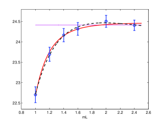
Figure 1: 4-loop plaquette vs $mL$ at fixed mass ($m=0.2$): the solid and the dashed lines correspond to different combinations of a constant plus a sum of negative exponentials and negative powers of $mL$; the horizontal line fits a constant.

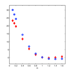
Figure 2: Infinite-volume 4-loop plaquette vs $m$: circles still contain $\ln(m)$ while diamonds are obtained after its subtraction (cf. eq. (7)).

5 Renormalization and improvement in the Electrostatic sector: setup

The EQCD action in the continuum is given by

$$S_{E}=\int\!{\rm d}^{d}x\,\biggl{\{}\frac{1}{2}\mathop{\textrm{Tr}}[F_{ij}^{2}(x)]+\mathop{\textrm{Tr}}[D_{i},A_{0}(x)]^{2}+m^{2}\mathop{\textrm{Tr}}[A_{0}^{2}(x)]+\lambda\big{(}\mathop{\textrm{Tr}}[A_{0}^{2}(x)]\big{)}^{\!2}\biggr{\}}~{},$$ (15)

where $F_{ij}(x)$ is the 3d field strength tensor, $D_{i}$ the covariant derivative and $A_{0}=\sum_{B=1}^{8}A_{0}^{B}T^{B}$, with $T^{B}$ normalised as before. Once again the strategy is to obtain the ${\overline{\mbox{\rm MS}}}$ scheme result starting from lattice measurements. Apart from the plaquette expectation value, this theory has however more condensates that play a role. In particular, derivatives with respect to the dimensionless variables $y$ and $x$, defined as $y=m^{2}/g_{E}^{4}$, $x=\lambda/g_{E}^{2}$ (with $g_{E}$ the EQCD gauge coupling), produce condensates quadratic and quartic in $A_{0}$ [10]. Subtracting the proper counterterms [21], and ${O}(a)$ or ${O}(a^{2})$ effects, which become important in the range of large $y$ where connection to the weak-coupling expansion can be made, we can extrapolate to the continuum, and finally obtain the pressure by integration [10].

The EQCD lattice action is given by

$$\nolinebreak\begin{array}[]{ccl}S_{\mbox{\scriptsize latt}}&=&\beta\sum_{x,~{}\!i<j}\Bigl{(}1-\frac{1}{3}\mathop{\textrm{Re}}\mathop{\textrm{Tr}}\big{[}P_{ij}(x)\big{]}\Bigr{)}-2\sum_{x,~{}\!i}\mathop{\textrm{Tr}}\big{[}\phi(x)~{}\!U_{i}(x)~{}\!\phi(x+i)~{}\!U_{i}^{{\dagger}}(x)\big{]}+\\ &+&\sum_{x}\bigg{\{}\alpha(\beta,\lambda,y_{\mbox{\scriptsize latt}})\mathop{\textrm{Tr}}\big{[}\phi^{2}(x)\big{]}+\lambda\Big{(}\!\mathop{\textrm{Tr}}\big{[}\phi^{2}(x)\big{]}\Big{)}^{2}\bigg{\}}~{},\end{array}$$ (16)

where now $\beta=2N_{\rm c}/ag_{E}^{2}$, $U_{i}$ is the link variable, $\phi=A_{0}\sqrt{6/\beta}$, and [21]

$$\nolinebreak\begin{array}[]{ccl}\alpha(\beta,\lambda,y_{\mbox{\scriptsize latt}})&=&6\bigg{\{}1+\frac{1}{6}y_{\mbox{\scriptsize latt}}-(6+\frac{5}{3}\lambda\beta)\frac{3.175911525625}{4\pi\beta}-\\ &-&\frac{3}{8\pi^{2}\beta^{2}}\Big{[}(10\lambda\beta-\frac{5}{9}\lambda^{2}\beta^{2})(\ln\beta+0.08849)+\frac{34.768}{6}\lambda\beta+36.130\Big{]}\bigg{\}}~{}.\end{array}$$ (17)

The first condensate we want to measure is the derivative with respect of $y_{\mbox{\scriptsize latt}}$: apart from a rescaling factor, it is equal to $\langle\mathop{\textrm{Tr}}[A_{0}^{2}]\rangle$ whose lattice counterpart has a perturbative expansion given by

$$\begin{array}[]{ccl}\langle~{}\!\mathop{\textrm{Tr}}~{}\![~{}\!\phi^{2}]~{}\!\rangle&=&d_{00}+d_{10}\frac{1}{\beta}+d_{11}\lambda+d_{20}\frac{1}{\beta{{}^{2}}}+d_{21}\frac{\lambda}{\beta}+d_{22}\lambda^{2}+\\ &+&d_{30}\frac{1}{\beta{{}^{3}}}+d_{31}\frac{\lambda}{\beta{{}^{2}}}+d_{32}\frac{\lambda^{2}}{\beta}+d_{33}\lambda^{3}+{O}\big{(}\frac{\lambda^{n}}{\beta{{}^{4-n}}}\big{)}~{}.\end{array}$$ (18)

These include the counterterms and lattice artifacts mentioned above: some of the coefficients ($d_{00}$, $d_{10}$, $d_{11}$, $d_{21}$, $d_{22}$) have already been estimated while the other ones (especially $d_{20}$ and $d_{30}$) are what we aim at computing by means of NSPT. We will again measure the observable for different values of the lattice extent $L$ and the parameters $\ln\beta$ and $y_{\mbox{\scriptsize latt}}$, and carry out an extrapolation in $L$ (at fixed $\ln\beta$ and $y_{\mbox{\scriptsize latt}}$) to get the infinite-volume results, from which we infer the behavior of the coefficients when varying the other variables.

6 Renormalization and improvement in the Electrostatic sector: first tests

The statistics we have collected so far is sufficient just to check the reliability of this approach. A first test is to compare our numerical estimates for the coefficient $d_{00}$ at fixed $L$ and $y_{\mbox{\scriptsize latt}}$ with the analytical results: this comparison is shown both in Table 2 and in Fig. 3 and appears satisfactory.

L	Exact result	NSPT estimate
5	0.6861	0.6867(11)
6	0.6833	0.6845(8)
7	0.6825	0.6837(6)
8	0.6822	0.6825(5)
9	0.6821	0.6822(4)
10	0.6821	0.6829(4)

Table 2: Comparison between exact and NSPT values of $d_{00}$, for $y_{\mbox{\scriptsize latt}}=1.0$.

As a second check, we inspect how our finite-volume data approach the infinite-volume limit at those orders for which we have a direct “exact” estimate of this limit: an example is given in Fig. 4 for the coefficient $d_{21}$ (whose infinite-volume value is 1.4072). Once again, the behavior looks encouraging; the same is observed for the terms not shown here.

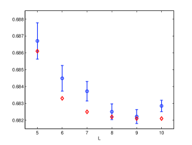
Figure 3: The coefficient $d_{00}$ vs $L$; exact (diamonds) and NSPT (circles) results.

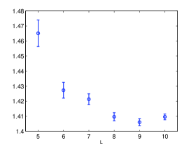
Figure 4: The coefficient $d_{21}$ vs $L$. The expected infinite-volume value is $1.4072$.

7 Conclusions and prospects

While our determination of the renormalization constant related to the ${O}(g^{6})$ contribution to the QCD pressure from the Magnetostatic sector has recently been completed [13], there is still work to do as regards the Electrostatic contributions. It is important to finalise this task, since the EQCD result has a wider range of applicability than the MQCD result alone. The first tests have produced encouraging results, so that there is every reason to believe that the determination of the most important new coefficients ($d_{20}$ and $d_{30}$) is also feasible, at least in a certain range of $y_{\mbox{\scriptsize latt}}$. With these results, the program initiated in ref. [10] could finally be carried out to completion.

References

- [1] P. Ginsparg, Nucl. Phys. B 170, 388 (1980); T. Appelquist and R.D. Pisarski, Phys. Rev. D 23, 2305.
- [2] K. Kajantie, M. Laine, K. Rummukainen and M. Shaposhnikov, Nucl. Phys. B 458, 90 (1996).
- [3] E. Braaten and A. Nieto, Phys. Rev. D 53, 3421 (1996).
- [4] P. Arnold and C. Zhai, Phys. Rev. D 50, 7603 (1994); ibid. 51, 1906 (1995).
- [5] G. Boyd et al., Nucl. Phys. B 469, 419 (1996).
- [6] A.D. Linde, Phys. Lett. B 96, 289 (1980).
- [7] A. Hietanen, K. Kajantie, M. Laine, K. Rummukainen and Y. Schröder, JHEP 01, 013 (2005).
- [8] K. Kajantie, M. Laine, K. Rummukainen and Y. Schröder, Phys. Rev. D 67, 105008 (2003).
- [9] M. Laine and Y. Schröder, Phys. Rev. D 73, 085009 (2006).
- [10] K. Kajantie, M. Laine, K. Rummukainen and Y. Schröder, Phys. Rev. Lett. 86, 10 (2001).
- [11] G. Parisi and Y.S. Wu, Sci. Sin. 24, 483 (1981).
- [12] F. Di Renzo, E. Onofri, G. Marchesini and P. Marenzoni, Nucl. Phys. B 426, 675 (1994).
- [13] F. Di Renzo, M. Laine, V. Miccio, Y. Schröder and C. Torrero, JHEP 07, 026 (2006).
- [14] A. Hietanen and A. Kurkela, hep-lat/0609015.
- [15] Y. Schröder, Nucl. Phys. B (Proc. Suppl.) 129, 572 (2004).
- [16] Y. Schröder and A. Vuorinen, hep-ph/0311323.
- [17] U.M. Heller and F. Karsch, Nucl. Phys. B 251, 254 (1985).
- [18] F. Di Renzo, A. Mantovi, V. Miccio and Y. Schröder, JHEP 05, 006 (2004).
- [19] H. Panagopoulos, A. Skouroupathis and A. Tsapalis, Phys. Rev. D 73, 054511 (2006).
- [20] H.J. Rothe, Lattice gauge theories: an introduction, World Sci. Lect. Notes Phys. 74, 1 (2005).
- [21] M. Laine and A. Rajantie, Nucl. Phys. B 513, 471 (1998).