CERN-PH-TH/2006-192

Lattice Gauge Theory Approach to Spontaneous

Symmetry Breaking from an Extra Dimension

Nikos Irges

Department of Physics and Institute of Plasma Physics,

University of Crete, GR-710 03 Heraklion, Crete, Greece

e-mail: irges@physics.uoc.gr

Francesco Knechtli

CERN, Physics Department, TH Division, 1211 Geneva 23, Switzerland

e-mail: knechtli@mail.cern.ch

 

Abstract

We present lattice simulation results corresponding to an $SU(2)$ pure gauge theory defined on the orbifold space $E_{4}\times I_{1}$, where $E_{4}$ is the four-dimensional Euclidean space and $I_{1}$ is an interval, with the gauge symmetry broken to a $U(1)$ subgroup at the two ends of the interval by appropriate boundary conditions. We demonstrate that the $U(1)$ gauge boson acquires a mass from a Higgs mechanism. The mechanism is driven by two of the extra-dimensional components of the five-dimensional gauge field which play respectively the role of the longitudinal component of the gauge boson and a massive real physical scalar, the Higgs particle. Despite the non-renormalizable nature of the theory, we observe only a mild cut-off dependence of the physical observables. We also show evidence that there is a region in the parameter space where the system behaves in a way consistent with dimensional reduction.

 

1 Introduction

Spontaneous symmetry breaking (SSB) is the phenomenon where the ground state of a system does not access all of its available symmetry, apparently breaking the symmetry group to a subgroup. In the Standard Model (SM) this is a crucial mechanism and it is not only responsible for predicting the existence of a fundamental scalar field, the Higgs particle, but also for the gauge bosons and fermions acquiring a mass. The somewhat unsatisfactory fact about this mechanism in the SM, is that the Higgs potential, which is the concrete object that drives SSB, is input by hand at tree level in the Lagrangian, simply because we do not have any more fundamental way to generate it. There are many ideas of course trying to suggest an origin for the Higgs and its potential, one of the most elegant being that the Higgs field is the extra dimensional component of a higher dimensional gauge field and that the potential is generated quantum mechanically [?]. The earliest scenarios considered as extra-dimensional space the sphere $S^{2}$ [?,?,?,?]. In later applications the extra-dimensional space was taken to be non-simply connected, like $S^{1}$ or $T^{2}$ [?,?,?], so that the (non-contractible) Polyakov loops are non-trivial. This is the general context where we would like to put ourselves in the present work. Alternative ways to achieve SSB in gauge theories with extra dimensions are discussed in [?,?–?].

There are enough motivations to take this idea seriously besides the economic way of generating the Higgs with its potential but the property that drew a lot of recent attention to these theories is the so claimed attractive possibility of all order finiteness of the physical scalar mass. This sounds like a paradox from the beginning since the very point which has kept many field theorists rather hesitant from taking such an idea seriously is that higher (than four) dimensional gauge theories are non-renormalizable and in a typical non-renormalizable theory one would expect that a mass parameter receives quantum corrections appearing in an arbitrary power of some dimensionless quantity built out of a dimensionful coupling and the cut-off. This is to be compared with the renormalizable SM where the couplings are dimensionless and the Higgs mass receives only a quadratic ultra-violet (UV) cut-off dependence under quantum corrections. Since even this quadratic UV sensitivity has been viewed as a drawback, supersymmetric generalizations of the SM were introduced and analyzed in detail, where the power like cut-off sensitivity is not present due to cancellations of infinities between superpartners. There is no doubt that supersymmetry is an elegant solution to the problem but it could happen that it is not realized at energies accessible in near future collider experiments so it is useful to be aware of alternative solutions. Back then to extra dimensions, in the case where the extra (fifth here) dimension is compactified on a circle, one can carry out a one-loop calculation of the Higgs mass and verify its aforementioned finiteness [?,?] and can even give all order arguments to that effect [?–?,?,?,?,?,?,?,?], but the problem with this solution is that a simple circle compactification can not be realistic for various reasons, the absence of chiral fermions being one of the main.

A way out is to compactify the extra dimension on an interval $I_{1}$ instead of a circle, which can support chiral fermions at the two ends of the interval. Since the interval can be obtained easily from the circle by ”orbifolding”, i.e. by identifying points and fields in the circle theory under the $Z_{2}$ reflection operator ${\cal R}:x^{5}\longrightarrow-x^{5}$, we will use the name orbifold when we refer to such a theory. A characteristic property of this orbifold is that it is defined on a space with two four dimensional boundaries at each of the fixed points of the reflection action, where the gauge symmetry is reduced, thus naturally differentiating the boundaries from the rest of the space, which we call the bulk. An unfortunate consequence of field theories defined in such spaces is that the all order finiteness of the Higgs mass arguments are not anymore applicable because of the bulk-boundary interactions appearing at higher orders in perturbation theory which start to infect the finite bulk mass with cut-off dependence [?]. This is not unexpected; it is known that handling non-renormalizable theories analytically is not easy, in fact there is no general prescription that can be used in these theories such that their predictions are trustworthy.

We would therefore like here to start a systematic investigation of higher dimensional orbifold gauge theories from the point of view of a lattice regularization [?,?,?]. The theory which will serve as our concrete example is an $SU(2)$ gauge theory which has the symmetry broken (by boundary conditions) to its $U(1)$ subgroup on the boundaries. This, we will argue, is a promising way of approaching extra dimensional theories: the goal is a non-perturbative understanding of a class of non-renormalizable theories and the hope is a non-perturbative understanding of the SM Higgs mechanism.

It turns out that phenomenology puts surprisingly tight constraints on models and we will concentrate here on the two most immediate ones as one proceeds with the construction. One is associated with the mere existence of a four dimensional effective action and the second, closely related to SM phenomenology, the expected hierarchy of masses between the physical Higgs and the massive gauge bosons in the broken phase of the SM.

1.1 Dimensional reduction

The first issue is to show that an extra dimensional theory possesses in its parameter space a regime where it undergoes some kind of effective dimensional reduction. This can happen, in principle, in more than one ways. Historically, the first mechanism of hiding the extra dimension is going to the ”Kaluza-Klein gauge” and making the size of the extra dimension small enough, so that its effects are negligible up to a certain energy scale and at the same time keeping the couplings perturbative so that the resulting effective theory can be useful for electroweak (or gravitational) physics. This is of course guaranteed as long as one treats the radius of the circle $R$, the cut-off $\Lambda$ and the gauge coupling $g_{5}$ as independent parameters which is perhaps justified to a certain extent – it depends essentially on how far one is willing to go in perturbation theory. In a non-perturbative formulation on the other hand it becomes right away obvious that these three parameters are tightly connected from the beginning and depending on where one sits in parameter space, a small change in one of the parameters could result in a dramatic change of the system. From this point of view, the region in parameter space where the theory describes the real world, (if it exists) could be only a small patch, which makes one wonder whether the free stretching of the dimensionful parameters sometimes employed to make a model phenomenologically viable is a valid operation.

More recently, mechanisms of dimensional reduction which depend on localization rather than compactification have been proposed. In the context of gauge theories, all of these mechanisms involve one way or another a strong coupling and therefore non-perturbative physics. One, is the so called layered phase originally proposed in [?]. The idea is to investigate a five-dimensional lattice model where the gauge coupling in the four dimensional slices along the extra dimension is different from the gauge coupling that describes the interaction between the slices. This anisotropy could give rise to a new, so-called layered, phase where the static force is of Coulomb type in the four-dimensional slices and confining along the extra dimension, thus providing a localization mechanism. Some evidence for the existence of the layered phase in Abelian gauge theory was recently given in [?]. Another similar idea was due to [?] where it is assumed that the system has a phase where the bulk is in a confined while the boundary (defined by a domain wall) is in a deconfined phase, which forces the boundary gauge fields to remain localized. This idea was investigated on the lattice [?] and it was found that the low-energy effective theory contains not only the localized zero-modes but also higher Kaluza–Klein modes.

A different mechanism of dimensional reduction was proposed in the context of the D-theory regularization of non-Abelian gauge theories [?,?,?]. Here a non-Abelian gauge theory in five dimensions arises as a low-energy effective description of a five-dimensional quantum link model. The size $L$ of four dimensions is taken to be infinity and the fifth dimension has a finite size $R$. If the five-dimensional theory happens to be in the Coulomb phase, the gluons are not massless but gain a mass which is exponentially small in the size of the extra-dimension. Thus by making $R$ larger the correlation length given by the inverse gluon mass grows exponentially fast in $R$ and therefore the extra-dimension disappears.

In this paper we will not be able to give a conclusive answer to this important issue since it would involve a very extensive scan of the parameter space. We will give though some indirect evidence for dimensional reduction in the orbifold theory and we will leave the question of which mechanism is responsible for it, for a future work. At a qualitative level, we will be able to map the part of the parameter space of our model where simulations were carried out onto the phase diagram of a known and well understood four dimensional theory, the Abelian Higgs model, which provides our first indirect evidence for an effective dimensional reduction. Our more quantitative, but still indirect, evidence for dimensional reduction will be the measurement of the static potential between two infinitely heavy charged particles placed on four-dimensional slices located at the origin and in the middle of the fifth-dimension, separated by a distance $r$. Using the fact that we measure a massive $U(1)$ gauge boson, we will fit the numerical data for the static potential to a five dimensional Yukawa potential and to a four dimensional Yukawa potential and compare the fits in both cases.

1.2 Hierarchy of masses

A universal feature that perturbative five dimensional orbifold pure gauge theories seem to posses is that the gauge bosons that survive on the boundaries are all massless and the mass of the Higgs turns out to be too low. In order to make some of the gauge bosons heavy one is forced to introduce fermions in the bulk [?], but still the ratio of the Higgs to the gauge boson mass is ${m_{h}}/{m_{\gamma}}<<1$ [?,?] and thus phenomenologically excluded, unless additional assumptions are made. This property has been traced to the fact that since in five dimensions gauge invariance forbids a tree level Higgs mass, it has to be generated quantum mechanically. This one-loop mass turns out to be suppressed compared to the gauge boson mass which is governed by a vacuum expectation value of order one. More concretely, at one loop, the Higgs mass is found to be $m_{h}\sim g_{5}/R^{3/2}$, where $g_{5}$ is the five-dimensional gauge coupling, whereas the gauge boson mass is basically $m_{\gamma}\sim\alpha/R$ where $\alpha$ is a dimensionless vacuum expectation value obtained from minimizing the potential (see Appendix A). Realistic models require a very small $\alpha$ even though typical one-loop potentials tend to yield an $\alpha$ which is either zero or of order $\sim 0.1$.

We will be able to compute the ratio $m_{h}/m_{\gamma}$ non-perturbatively and find that, contrary to perturbative expectations, a Higgs mechanism is at work, resulting into a non-zero gauge boson mass, for a large part of the parameter space (in fact for the whole range of parameters we were able to scan). Again, disentangling the precise dependence of this ratio on compactification and finite lattice size effects requires a larger scan of the parameter space, which will be the topic of a future work.

1.3 Organization of the paper

In this paper we investigate numerically a one dimensional subspace of the parameter space of a five dimensional lattice gauge theory, starting from the vicinity of a first order phase transition and approaching the perturbative domain. In section 2, using generic properties of the measured orbifold spectrum, we argue that the spectrum of the system in part of this region seems to be consistent with an effective dimensional reduction. In section 3 we construct in detail the lattice regulated theory and in particular its observables. In section 4 we present in detail our quantitative evidence for spontaneous symmetry breaking and dimensional reduction. In section 5 we state our conclusions. Finally, for completeness we provide two detailed appendices with some background, appendix A on 1-loop results and B on the derivation of the five-dimensional Yukawa potential.

2 The orbifold effective theory

We consider a pure $SU(2)$ Yang–Mills (YM) theory in five dimensions with gauge potential $A_{M}$, $M=0,1,2,3,5$. The fifth dimension is an interval, obtained by identifying points and fields on a circle of radius $R$ under the $Z_{2}$ reflection operator ${\cal R}:x^{5}\longrightarrow-x^{5}$. The projection breaks the gauge symmetry at the two ends of the interval according to

$$SU(2) \longrightarrow U(1)\,.$$ (2.1)

In the picture of dimensional reduction as it is known in finite temperature field theory [?–?] the five-dimensional fields are expanded in a Fourier series in the quantized momentum along the compact dimension. At low energies, in our case much below the compactification scale given by the inverse radius $1/R$, we have an effective four-dimensional theory of the zero-modes (i.e. constant along the fifth dimension) of the fields.

But the Fourier series that defines the Kaluza–Klein expansion breaks gauge invariance. This we cannot afford at the non-perturbative level. Here the particle spectrum is read off from correlations of five-dimensional, gauge invariant operators. These operators are classified according to specific symmetries. If dimensional reduction occurs, a mass gap in the various particle channels should be seen. The ground state of the operators which corresponds to the $A_{5}$ gauge field component has the quantum numbers of a complex scalar and the ground state of the $A_{\mu},\mu=0,1,2,3$ components have quantum numbers of a $U(1)$ gauge field from the point of view of four dimensions. Clearly, the lowest lying spectrum of the orbifold theory should coincide with the one of the four-dimensional Abelian Higgs model, if dimensional reduction works like in finite temperature field theory. The spectra with the higher excitations included will be different, as in the five-dimensional theory they are sensitive to the compactification scale $1/R$. Before defining the orbifold theory in great detail and present extensive simulation results (which will be the topic of the next sections), one would hope to be able to exploit this similarity of spectra by mapping the phase diagram of the orbifold simulation on the phase diagram of the Abelian Higgs model. Being able to do so, would be a first circumstantial evidence for an effective dimensional reduction.

Next, we define the parameter space of our model. In a lattice regularization, the cut-off is provided by the inverse lattice spacing $\Lambda=a^{-1}$ and it preserves gauge invariance. That is why the lattice formulation is particularly useful to study non-renormalizable theories, which requires a cut-off. The parameter space of the lattice theory is two dimensional . One of the parameters is the (dimensionless) number of lattice points in the fifth dimension

$$N_{5} = \frac{\pi R}{a}$$ (2.2)

and the second is the dimensionless five dimensional lattice coupling

$$\beta=\frac{2N}{g_{5}^{2}}a=\frac{2N}{g_{0}^{2}}\,,$$ (2.3)

where $g_{0}$ is the dimensionless bare gauge coupling. For later reference, notice that in regions of the parameter space where $g_{5}$ has a mild cut-off dependence, $\beta$ is inversely proportional to $\Lambda$. All observables are computed in units of the lattice spacing, or equivalently in units of $R$, and are thus functions of $N_{5}$ and $\beta$. One can also define a derived parameter, the coupling

$$\beta_{4}^{eff}\equiv\frac{1}{g_{4}^{2}}=\frac{\pi R}{g_{5}^{2}},$$ (2.4)

for the effective four-dimensional theory. It is also possible in principle to use an anisotropic lattice [?] in which case a lattice gauge coupling (and a different lattice spacing) is defined for the fifth dimension ($\beta_{5}$) and a different one for the four dimensional subspace ($\beta_{4}$). Here we will restrict ourselves to isotropic lattices for which $\beta_{4}=\beta_{5}=\beta$.

From simulations of the five dimensional $SU(2)$ gauge theory on the orbifold $S^{1}/\mathbb{Z}_{2}$ with the number of points in the extra dimension fixed to $N_{5}=4$, and on an isotropic lattice with an associated coupling $\beta$, the spectrum can be safely determined when $\beta$ is larger than a critical value $\beta_{c}=1.5975$, which separates a confined ($\beta<\beta_{c}$) from a deconfined ($\beta>\beta_{c}$) phase. The spectrum measured in simulations corresponding to the deconfined phase consists of a massive Higgs ground state and a massive Abelian gauge boson, along with their excitations [?] which implies that our system in this region of parameter space crosses from a confined phase into a Higgs phase. In order to be able to make a comparison with the Abelian Higgs model we now recall a few well known facts.

We summarize results from analytic [?,?] and numerical [?] studies of the four dimensional Abelian Higgs model. The Euclidean action may be written as

$$S = \sum_{x}\Bigg{\{}\lambda(\phi^{\dagger}(x)\phi(x)-1)^{2}+\phi^{\dagger}(x)\phi(x)$$ (2.5)

$$-\kappa\sum_{\mu}\left(\phi^{\dagger}(x){\rm e}^{iqA_{\mu}(x)}\phi(x+a\hat{\mu})+{\rm c.c.}\right)\Bigg{\}}-\frac{\beta}{2}\sum_{p}U_{p}\,.$$

Here, $\phi(x)$ is the complex Higgs field, $q$ is its charge and $\kappa$ the hopping parameter related to the bare mass $m_{0}$ through

$$a^{2}m_{0}^{2} = \frac{1-2\lambda}{\kappa}-8\,.$$ (2.6)

The analytic study in [?] was performed in the limit $\lambda\to\infty$ where the length of the Higgs field $\rho$ is frozen to 1. In the unitary gauge the action then reads

$$S = -\kappa\sum_{\mu}2\cos[qA_{\mu}(x)]-\frac{\beta}{2}\sum_{p}U_{p}\,.$$ (2.7)

There are two interesting cases. One is when the Higgs field is in the fundamental representation, that is it has charge $q=1$ and the second is when it has charge $q=2$. For us it is the second case that is relevant since, as will show in the next section, the lattice operator which is identified with the Higgs has charge two.

Figure 1: Phase diagram of the Abelian Higgs model for the Higgs field with charge $q=2$. From studies at $\lambda=\infty$ [?].

We inspect the action for $\lambda=\infty$ in the unitary gauge, Eq. (2.7), in the limit $\kappa\to\infty$. In this limit the gauge variable $A_{\mu}(x)$ can take, for $q=2$, two values, 0 or $\pi$, corresponding to $\mathbb{Z}_{2}$ gauge links $U(x,\mu)=\pm 1$. (For general charge $q$ it will be a $\mathbb{Z}_{q}$ gauge theory). The $\mathbb{Z}_{2}$ gauge theory has a second order phase transition. The analytic study of [?] in the $\lambda=\infty$ case concludes that there are three distinct phases, sketched in Fig. 1. The main difference compared to the $q=1$ case is a phase boundary that separates the Higgs from the confinement phase. The static potential in the Higgs phase is of Yukawa type. In the confinement phase it rises linearly (area law for Wilson loops) which is not the case in the confinement region for a fundamental Higgs.

Clearly, this is the version of the Abelian Higgs model on which the orbifold theory can be naturally mapped since the lowest lying spectra are the same and the part of the orbifold phase diagram we have investigated can be recognized inside the phase diagram of the $q=2$ Abelian Higgs model.

3 Orbifold on the lattice

Gauge theories on the orbifold can be discretized on the lattice [?,?]. One starts with a gauge theory formulated on a five-dimensional torus with lattice spacing $a$ and periodic boundary conditions in all directions $M=0,1,2,3,5$. The spatial directions ($M=1,2,3$) have length $L$, the time-like direction ($M=0$) has length $T$, and the extra dimension ($M=5$) has length $2\pi R$. The coordinates of the points are labelled by integers $n\equiv\{n_{M}\}$ and the gauge field is the set of link variables $\{U(n,M)\in SU(N)\}$. The latter are related to a gauge potential $A_{M}$ in the Lie algebra of $SU(N)$ by $U(n,M)=\exp\{aA_{M}(n)\}$. Embedding the orbifold action in the gauge field on the lattice amounts to imposing on the links the $\mathbb{Z}_{2}$ projection

$$(1-\Gamma)U(n,M)=0\,,$$ (3.8)

where $\Gamma={\cal R}{\cal T}_{g}$. Here, ${\cal R}$ is the reflection operator that acts as ${\cal R}\,n=(n_{\mu},-n_{5})\equiv{\bar{n}}\;(\mu=0,1,2,3)$ on the lattice and as ${\cal R}\,U(n,\mu)=U({\bar{n}},\mu)$ and ${\cal R}\,U(n,5)=U^{\dagger}({\bar{n}}-{\hat{5}},5)$ on the links. The group conjugation ${\cal T}_{g}$ acts only on the links, as ${\cal T}_{g}U(n,M)=gU(n,M)g^{-1}$, where $g$ is a constant $SU(N)$ matrix with the property that $g^{2}$ is an element of the centre of $SU(N)$. For $SU(2)$ we will take $g=-i\sigma^{3}$. Only gauge transformations $\{\Omega(n)\}$ satisfying $(1-\Gamma)\Omega=0$ are consistent with Eq. (3.8). This means that at the orbifold fixed points, for which $n_{5}=0$ or $n_{5}=N_{5}$, the gauge group is broken to the subgroup that commutes with $g$. For $SU(2)$ this is the $U(1)$ subgroup parametrized by $\exp(i\phi\sigma^{3})$, where $\phi$ are compact phases.

After the projection in Eq. (3.8), the fundamental domain is the strip $I_{1}=\{n_{\mu},0\leq n_{5}\leq N_{5}\}$. The gauge-field action on $I_{1}$ is taken to be the Wilson action

$$S_{W}^{\rm orb}[U]=\frac{\beta}{2N}\sum_{p}w(p)\;{{\rm tr}}\,\{1-U(p)\},$$ (3.9)

where the sum runs over all oriented plaquettes $U(p)$ in $I_{1}$. The weight $w(p)$ is 1/2 if $p$ is a plaquette in the $(\mu\nu)$ planes at $n_{5}=0$ and $n_{5}=N_{5}$, and 1 in all other cases. Dirichlet boundary conditions are imposed on the gauge links

$$U(n,\mu) = g\,U(n,\mu)\,g^{-1}\quad\mbox{at $n_{5}=0$ and $n_{5}=N_{5}$.}$$ (3.10)

The gauge variables at the boundaries are not fixed but are restricted to the subgroup of $SU(N)$, invariant under ${\cal T}_{g}$. The Wilson action together with these boundary conditions reproduce the correct naive continuum gauge action and boundary conditions on the components of the five-dimensional gauge potential [?]. For example, for $SU(2)$, $A_{\mu}^{3}$ (“photon”) and $A_{5}^{1,2}$ (“Higgs”) satisfy Neumann boundary conditions and $A_{\mu}^{1,2}$ and $A_{5}^{3}$ Dirichlet ones.

One of the main results of [?] was to show, through a geometrical construction, that the orbifold projection equation Eq. (3.8) implies the absence of a boundary counterterm for the Higgs mass. Given the explicit breaking of the gauge invariance at the boundaries, a boundary mass term for $A_{5}$ is invariant under the unbroken gauge group. In the continuum this mass term would be ${\rm tr}\{[A_{5},g][A_{5},g^{-1}]\}$ evaluated at the boundaries $x_{5}=0$ and $x_{5}=\pi R$. If present, such a term would imply a quadratic sensitivity of the Higgs mass to the cut-off. For the lattice action Eq. (3.9) this would require to add a boundary action term with an additional coefficient $\tilde{\mu}$. As the lattice spacing $a$ changes, a fine tuning of $\tilde{\mu}$ would be required to keep the Higgs mass finite. Fortunately this term is absent and the orbifold action is simply Eq. (3.9). Since five-dimensional theories are non-renormalizable, they make sense only as effective theories for energy scales much below the cut-off. On the lattice this is the Symanzik effective action [?,?,?,?], a continuum action which is a systematic expansion in the lattice spacing $a$. For the orbifold theory the Symanzik effective action is [?]

$$S = -\frac{1}{2g_{5}^{2}}\Bigg{[}\int{\rm d}^{5}z\,{\rm tr}\{F_{MN}F_{MN}\}$$ (3.11)

$$+ab_{1}\int_{z=\{0,\pi R\}}{\rm d}^{4}x\,{\rm Re}\,{\rm tr}\{gF_{MN}F_{MN}\}+ab_{2}\int_{z=\{0,\pi R\}}{\rm d}^{4}x\,{\rm Re}\,{\rm tr}\{gF_{MN}gF_{MN}\}$$

$$+a^{2}c\int{\rm d}^{5}z\,{\rm tr}\{D_{L}F_{MN}D_{L}F_{MN}\}+\ldots\Bigg{]}\,,$$

where $F_{MN}$ is the field strength tensor, $D_{L}$ its covariant derivative and the coefficients $b_{1},b_{2},c,\ldots$ are computable in perturbation theory. At 1-loop, $b_{1}\neq 0$ and $b_{2}=0$ [?]. A boundary mass term for the Higgs would appear with a coefficient $\tilde{\mu}/a^{2}$.

3.1 Operators for the Higgs

If the fifth dimension were infinite, the gauge links $U(n,5)$ would be gauge-equivalent to the identity, which corresponds to the continuum axial gauge $A_{5}\equiv 0$. On the circle $S^{1}$ one can gauge-transform $U(n,5)$ to an $n_{5}$-independent matrix $V(n_{\mu})$ that satisfies $P=V^{2N_{5}}$, where $P=P(n_{\mu})$ is the Polyakov line winding around the extra dimension at four-dimensional location $n_{\mu}$. Therefore an extra-dimensional potential $(A_{5})_{\rm lat}$ can be defined on the lattice, through $V=\exp\{a(A_{5})_{\rm lat}\}$, as

$$a(A_{5})_{\rm lat}=\frac{1}{4N_{5}}(P-P^{\dagger})+{\rm O}(a^{3})\,.$$ (3.12)

At finite lattice spacing the O($a^{3}$) corrections in Eq. (3.12) are neglected. One easily checks that ${\cal R}\,P\,=\,P^{\dagger}$ and so ${\cal R}\,(A_{5})_{\rm lat}=-(A_{5})_{\rm lat}$, as it should be to have the same transformation behaviour as $A_{5}$ in the continuum.

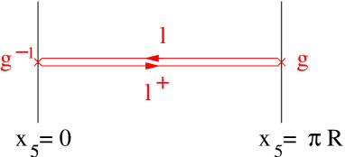
Figure 2: The Polyakov line $P$ on $S^{1}/\mathbb{Z}_{2}$.

In order to construct the gauge potential $A_{5}$ on the orbifold $S^{1}/\mathbb{Z}_{2}$ we start from the circle $S^{1}$ parametrized by the coordinates $n_{5}=-N_{5},\ldots,N_{5}-1$ ($N_{5}=\pi R/a$ is identified with $-N_{5}$). We impose on the links building the Polyakov line $P$

$$P(n_{\mu})\,=\,U((n_{\mu},0),5)\,\ldots\,U((n_{\mu},N_{5}-1),5)\,U((n_{\mu},-N_{5}),5)\,\ldots\,U((n_{\mu},-1),5)$$ (3.13)

the orbifold projection Eq. (3.8). The result is

$$P(n_{\mu}) = l(n_{\mu})\,g\,l^{\dagger}(n_{\mu})\,g^{-1}\,,$$ (3.14)

with

$$l(n_{\mu}) = U((n_{\mu},0),5)\,U((n_{\mu},1),5)\,\ldots\,U((n_{\mu},N_{5}-1),5)\,.$$ (3.15)

The Polyakov line Eq. (3.14) on $S^{1}/\mathbb{Z}_{2}$ is shown schematically in Fig. 2 and from it we define $(A_{5})_{\rm lat}(n_{\mu})=\{P(n_{\mu})-P^{\dagger}(n_{\mu})\}/(4N_{5})$. Being anti-Hermitian, the field $(A_{5})_{\rm lat}$ can be represented using the unit matrix and the Hermitian generators $T^{A}$ of $SU(N)$:

$$(A_{5})_{\rm lat} = -ig_{0}(A_{5}^{0}\,\mathbf{1}_{N}+A_{5}^{A}\,T^{A})\,.$$ (3.16)

In order to construct the Higgs field on $S^{1}/\mathbb{Z}_{2}$ we have to project $(A_{5})_{\rm lat}$ onto the components $A_{5}^{\hat{a}}$ for which $g\,T^{\hat{a}}\,g^{-1}=-T^{\hat{a}}$ (the other generators have $g\,T^{a}\,g^{-1}=T^{a}$). The Higgs field is now defined as in the continuum

$$\Phi(n_{\mu}) = [a(A_{5})_{\rm lat}(n_{\mu}),g]\,=\,2iag_{0}A_{5}^{\hat{a}}(n_{\mu})\,g\,T^{\hat{a}}\,.$$ (3.17)

Note that the commutator projects out the identity component of $(A_{5})_{\rm lat}$. Under gauge transformation $\Omega(n)$, $l(n_{\mu})\longrightarrow\Omega(n_{\mu},0)\,l(n_{\mu})\,\Omega(n_{\mu},N_{5})^{-1}$. Since $[\Omega(n),g]=0$ at the orbifold boundaries $n_{5}=0$ and $n_{5}=N_{5}$, it follows that

$$\Phi(n_{\mu}) \longrightarrow \Omega(n_{\mu},0)\,\Phi(n_{\mu})\,\Omega(n_{\mu},0)^{-1}\,.$$ (3.18)

The Higgs field $\Phi$ transforms like a field strength tensor at the boundary. In the special case of gauge group $SU(2)$ only a $U(1)$ gauge symmetry survives at the boundaries. If we parameterize the $U(1)$ boundary gauge transformations by $\Omega(n_{\mu},0)=\exp\{i\omega(n_{\mu})\sigma^{3}\}$, the Higgs field transforms as

$$\Phi\,=\,\left(\begin{array}[]{cc}0&h=\phi_{1}-i\phi_{2}\\ h^{\dagger}=\phi_{1}+i\phi_{2}&0\end{array}\right) \longrightarrow \left(\begin{array}[]{cc}0&{\rm e}^{2i\omega}h\\ {\rm e}^{-2i\omega}h^{\dagger}&0\end{array}\right)\,.$$ (3.23)

showing that it has charge 2 under the $U(1)$ gauge group.

Since ${\rm tr}\{\Phi\}=0$, in order to extract the Higgs mass we define

$$H(n_{0}) = \left(\frac{a}{L}\right)^{3}\sum_{n_{1},n_{2},n_{3}}{\rm tr}\{\Phi(n_{\mu})\,\Phi^{\dagger}(n_{\mu})\}$$ (3.24)

and build the connected correlation

$$C(t) = \frac{a}{T}\sum_{n_{0}}\left\{\langle H(n_{0})\,H(n_{0}+t/a)\rangle-\langle H(n_{0})\rangle\,\langle H(n_{0}+t/a)\rangle\right\}$$

$$\stackrel{{\scriptstyle t\to\infty}}{{\longrightarrow}} {\rm const.}\times{\rm e}^{-m_{h}t}\,,$$

and the Higgs mass $m_{h}$ can be extracted from the effective masses $am_{h,{\rm eff}}(t+a/2)\,=\,\ln\{C(t)/C(t+a)\}$. Writing the correlation $C(t)$ as

$$C(t) = \langle\left(H(t)-\langle H\rangle\right)\left(H(0)-\langle H\rangle\right)\rangle$$ (3.26)

one can see that it is a sum of positive and negative numbers of order one, the result being a small number due to cancellations. On the other hand, the variation

$$\Delta C = \langle\left(H(t)-\langle H\rangle\right)^{2}\left(H(0)-\langle H\rangle\right)^{2}\rangle-C^{2}$$ (3.27)

is a sum of positive numbers of order one minus a very small number and hence of order one. Furthermore, $\Delta C$ is essentially independent of $t$. This means that the error in the effective Higgs masses is approximately

$$\Delta am_{h,{\rm eff}} \simeq \Delta C\sqrt{\left(\frac{1}{C(t)}\right)^{2}+\left(\frac{1}{C(t+a)}\right)^{2}}\,,$$ (3.28)

and, since $C(t)\sim e^{-m_{h}t}$, its $t$–dependence is

$$\Delta am_{h,{\rm eff}} \sim e^{m_{h}t}.$$ (3.29)

In the above, $m_{h}$ is the plateau value of the Higgs mass which is constant and therefore one expects that the error in $m_{h}$ increases with $t$ exponentially.

3.1.1 Variational technique

It turns out that the correlation function Eq. (3.1) suffers from a loss of significance in numerical simulation. This is the, unfortunately, common problem of signals, which are exponentially small in the time $t$, with an almost constant variance, and hence constant statistical error. The ratio of the signal to the error falls off exponentially in the time $t$; in the large-$t$ region, where the leading exponential decay Eq. (3.1) due to the Higgs mass should be seen, the signal is lost. This is reflected in the exponentially growing error of the effective masses Eq. (3.29).

To cure this problem we employ the variational technique of [?]. A basis of Higgs operators is constructed and the best operator to capture the Higgs mass in Eq. (3.1), i.e. whose overlap with the eigenstate of the Hamiltonian is the largest, will be a linear combination of these basis fields. If the contributions from excited states are suppressed then the leading exponential Eq. (3.1) can be extracted at smaller values of $t$, where the signal might not be lost.

Here we sketch how this works; more details can be found in [?]. We construct a set of Euclidean fields $\mathcal{O}_{i}$, $i=1,\ldots,r$ with the same quantum numbers as $H\equiv\mathcal{O}_{1}$ in Eq. (3.24). Then we build the matrix correlation function

$$C_{ij}(t) = \langle\mathcal{O}_{i}(t)\mathcal{O}_{j}(0)^{*}\rangle-\langle\mathcal{O}_{i}(t)\rangle\,\langle\mathcal{O}_{j}(0)^{*}\rangle\,,$$ (3.30)

and write the spectral decompositions

$$\langle\mathcal{O}_{i}(t)\mathcal{O}_{j}(0)^{*}\rangle = \frac{1}{Z}\sum_{m,n}{\rm e}^{-E_{n}T-t(E_{m}-E_{n})}A_{nm}^{(i)}A_{nm}^{(j)\,*}\,$$ (3.31)

$$\langle\mathcal{O}_{i}(t)\rangle = \frac{1}{Z}\sum_{n}{\rm e}^{-E_{n}T}A_{nn}^{(i)}\,,$$ (3.32)

where

$$Z\,=\,\sum_{n}{\rm e}^{-E_{n}T} A_{mn}^{(i)}\,=\,\langle m|\mathcal{O}_{i}(0)|n\rangle\,.$$ and (3.33)

Here $m,n=0,1,2,...$ label the eigenstates $|m\rangle$ with energy eigenvalue $E_{m}$ of the Hamiltonian $\mathbb{H}$ and $T$ is the temporal size of the lattice. We use the same symbol $\mathcal{O}_{i}$ to denote the Euclidean field and the corresponding operator in the Hamiltonian formulation.

There are two effects, which derive from the finiteness of $T$ and the periodic boundary conditions in time (which imply taking the overall trace in the spectral decomposition) [?]. Firstly, if the operators $\mathcal{O}_{i}$ have a non-vanishing expectation value the connected correlation functions Eq. (3.30) have in general t-independent contributions

$${\rm e}^{-m_{h}T}\,\left[A_{00}^{(i)}-A_{11}^{(i)}\right]\,\left[A_{00}^{(j)}-A_{11}^{(j)}\right]^{*}\,,$$ (3.34)

where $m_{h}=E_{1}-E_{0}$ is the mass gap, i.e. the Higgs ground state mass.

Secondly, in the limit that $T$, $t$ are both large and the difference $T-t$ is close to $t$, the matrix correlation function Eq. (3.30) has the leading behavior

$$C_{ij}(t) \longrightarrow \sum_{n>0}\left[{\rm e}^{-(E_{n}-E_{0})t}+{\rm e}^{-(E_{n}-E_{0})(T-t)}\right]A_{n0}^{(i)}A_{n0}^{(j)\,*}+$$ (3.35)

$$\sum_{m,n>0}{\rm e}^{-(E_{n}-E_{0})T-(E_{m}-E_{n})t}A_{nm}^{(i)}A_{nm}^{(j)\,*}\,.$$

Here we have assumed that $A_{mn}=A_{nm}^{*}$ and $C_{ij}(t)$ is real, which is true if the operators $\mathcal{O}_{i}$ are Hermitian. If we take $t=T/2$, the contribution of the second term in Eq. (3.35) goes like $\exp\{-[(E_{n}+E_{m})/2-E_{0}]T\}$ compared to $\exp\{-(E_{n}-E_{0})T/2\}$ of the first term. The second term is hence subleading and can be neglected. We get

$$C_{ij}(t) \longrightarrow C_{ij}^{\prime}(t)+C_{ij}^{\prime}(T-t)\,,\quad C_{ij}^{\prime}(t)=\sum_{n>0}A_{n0}^{(i)}A_{n0}^{(j)\,*}{\rm e}^{-(E_{n}-E_{0})t}\,.$$ (3.36)

The correlation function is a sum of two contributions and is symmetric about $t=T/2$.

First we assume that $T$ is large enough so that the t-independent contribution Eq. (3.34) is negligible and that $t$ is small enough so that the contribution $T-t$ is also negligible. Then the correlations Eq. (3.30) have the $T=\infty$ behavior (assumed in [?])

$$C_{ij}(t) = \sum_{\alpha=1}^{\infty}A_{\alpha 0}^{(i)}A_{\alpha 0}^{(j)*}{\rm e}^{-tW_{\alpha}}\,,\quad W_{\alpha}=E_{\alpha}-E_{0}\,.$$ (3.37)

The lowest masses $W_{\alpha}$ can be extracted by solving the generalized eigenvalue problem

$$C(t)_{ij}\psi_{\alpha,j}(t,t_{0}) = \lambda_{\alpha}(t,t_{0})C_{ij}(t_{0})\psi_{\alpha,j}(t,t_{0})\,,$$ (3.38)

where the correlation matrix is taken at variable time $t$ and at fixed time $t_{0}$ (we may set $t_{0}=0$). From a mathematical lemma proved in [?] it follows that

$$\lambda_{\alpha}(t,t_{0}) \stackrel{{\scriptstyle t\to\infty}}{{=}}c_{\alpha}{\rm e}^{-tW_{\alpha}}\left[1+{\rm O}(e^{-t\Delta W_{\alpha}})\right]\,,\quad\alpha=1,\ldots,r\,,$$ (3.39)

where $c_{\alpha}>0$ and $\Delta W_{\alpha}=\min_{\beta\neq\alpha}|W_{\alpha}-W_{\beta}|$. One expects that $c_{\alpha}\simeq{\rm e}^{t_{0}W_{\alpha}}$ and that the coefficients of the correction terms in Eq. (3.39), because of the excited states, are suppressed. The masses can be extracted from

$$aW_{\alpha}(t+a/2) = \ln\left(\frac{\lambda_{\alpha}(t,t_{0})}{\lambda_{\alpha}(t+a,t_{0})}\right)$$ (3.40)

at moderately large value of $t$.

If the contribution $T-t$ is not negligible, as it happens when $t$ approaches $T/2$ (and we might be forced to go to such large values of $t$ to find a plateau), then a different formula has to be used. The starting point is Eq. (3.36). If we say that $\lambda_{\alpha}^{\prime}(t,t_{0})$ solves the generalized eigenvalue problem Eq. (3.38) for the matrix $C^{\prime}$ defined in Eq. (3.36), then it is straightforward to show that

$$\lambda_{\alpha}(t,t_{0}) = \lambda_{\alpha}^{\prime}(t,t_{0})+\lambda_{\alpha}^{\prime}(T-t,t_{0})$$ (3.41)

solves the generalized eigenvalue problem for the full matrix $C$. Using Eq. (3.39) for $\lambda^{\prime}$ we get the formula

$$\lambda_{\alpha}(t,t_{0}) = 2c_{\alpha}{\rm e}^{-W_{\alpha}T/2}\cosh[(T/2-t)W_{\alpha}]\,.$$ (3.42)

By using the ratio $r_{12}=\lambda_{\alpha}(t_{1},t_{0})/\lambda_{\alpha}(t_{2},t_{0})$ and the definitions

$$x={\rm e}^{-W_{\alpha}}\,, \tau_{1}=T/2-t_{1}\,, \tau_{2}=T/2-t_{2}\,,$$ (3.43)

it is easy to arrive at the equation

$$r_{12}\left(x^{\tau_{2}}+x^{-\tau_{2}}\right)-\left(x^{\tau_{1}}+x^{-\tau_{1}}\right) = 0$$ (3.44)

to be solved numerically (Newton-Raphson) for $x$. We take $t_{0}=0$, $t_{1}=t$ and $t_{2}=t+a$ for $t=a,2a,\ldots,T/2-a$.

3.1.2 Higgs operators

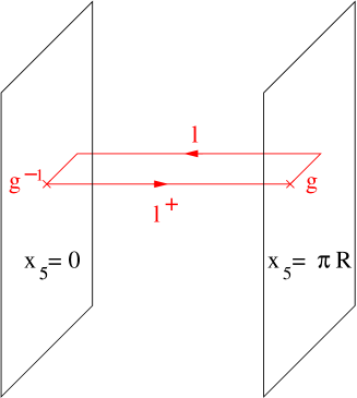
Figure 3: The displaced Polyakov line $L$ on $S^{1}/\mathbb{Z}_{2}$.

A basis of Higgs operators $\mathcal{O}_{i}=H_{i}$, defined as in Eq. (3.24), can be constructed by modifying the definition of the Higgs field $\Phi$ to create a set of fields $\Phi_{i}$. We can for example consider displaced Polyakov lines on $S^{1}/\mathbb{Z}_{2}$ as shown in Fig. 3. The position where the displacement in one of the spatial directions $k=1,2,3$ takes place can be varied along the extra coordinate $n_{5}=0,1,\ldots,\lfloor N_{5}/2\rfloor$. The displacements at the other $n_{5}$ values are equivalent by symmetry with respect to reflection $n_{5}\longrightarrow N_{5}-n_{5}$. For the displacement at $n_{5}=0$ Eq. (3.14) is replaced by

$$P^{(0)}(n_{\mu}) = \frac{1}{6}\sum_{\stackrel{{\scriptstyle n_{0}=n^{\prime}_{0}}}{{|n-n^{\prime}|=a}}}U(n_{\mu},n^{\prime}_{\mu})|_{n_{5}=0}\,l(n^{\prime}_{\mu})\,U^{\dagger}(n_{\mu},n^{\prime}_{\mu})|_{n_{5}=N_{5}}\,g\,l^{\dagger}(n_{\mu})\,g^{-1}\,,$$ (3.45)

and similar expressions $P^{(n_{5})}$ for $n_{5}=1,\ldots,\lfloor N_{5}/2\rfloor$. In Eq. (3.45) $U(n_{\mu},n_{\mu}^{\prime})$ is the parallel transporter from the four-dimensional point $n_{\mu}^{\prime}$ to $n_{\mu}$ in the indicated slice $n_{5}$ in the extra dimension.

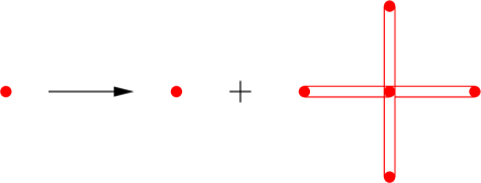
Figure 4: A smearing procedure for the Higgs field $\Phi$.

Yet another possibility to create fields for the variational basis is to consider smeared Higgs fields. The simplest is shown in Fig. 4: the field $\Phi(n_{\mu})$ (represented by a thick point) is replaced by a smeared field $\Phi^{\prime}(n_{\mu})$ made of a linear combination of $\Phi(n_{\mu})$ and the nearest neighbour fields in the three dimensional space

$$\Phi^{\prime}(n_{\mu}) = (1-\alpha)\,\Phi(n_{\mu})+\frac{\alpha}{6}\sum_{\stackrel{{\scriptstyle n_{0}=n^{\prime}_{0}}}{{|n-n^{\prime}|=a}}}U(n_{\mu},n_{\mu}^{\prime})|_{n_{5}=0}\,\Phi(n_{\mu}^{\prime})\,U^{\dagger}(n_{\mu},n_{\mu}^{\prime})|_{n_{5}=0}\,.$$ (3.46)

The smearing parameter is $\alpha$. The definition of Eq. (3.46) ensures that $\Phi^{\prime}$ transforms as $\Phi$ under the gauge transformation in Eq. (3.18). Variants of the smearing technique can be found in [?]. The smearing procedure Eq. (3.46) can be iterated a number of times, which we take to be 3. We set $\alpha=0.7$.

Finally, the gauge links used to construct all the Higgs fields $\Phi_{i}$ are replaced by smeared gauge links. This is a very simple procedure to create extended operators. We have implemented APE smearing [?] for the spatial links, i.e. $U(z,k)$, $k=1,2,3$ and $U(z,5)$. The links are decorated with staples in the spatial directions $l=1,2,3$, clearly with the restriction $l\neq k$ for $U(z,k)$. The smeared link $U^{\prime}$ is obtained by adding to $(1-\alpha)U$ the sum of the decorating staples multiplied by $\alpha$/(number of staples), where $\alpha$ is the smearing parameter. The smeared link is projected back onto $SU(2)$. The smearing of the gauge links is iterated 3 times with $\alpha=0.75$.

3.2 Photon operators

In this section we describe the construction of operators in the $SU(2)$ orbifold, which create the gauge boson (photon) associated with the unbroken $U(1)$ gauge group on the boundaries. For each Higgs field $\Phi_{i}$ constructed as described in Section 3.1.2 we define the $SU(2)$ valued quantity (in the following we suppress the index $i$)

$$\alpha(n_{\mu}) = \frac{\Phi(n_{\mu})}{\sqrt{\det(\Phi(n_{\mu}))}}\,.$$ (3.47)

We note that from Eq. (3.17) and $g^{\dagger}=-g$ (which holds for SU(2)) it follows $\alpha^{\dagger}=-\alpha$. For the three spatial directions $k=1,2,3$ we define a “decorated double link”

$$V(n_{\mu},k) = U(n_{\mu},k)\,\alpha(n_{\mu}+a{\hat{k}})\,U^{\dagger}(n_{\mu},k)\,\alpha(n_{\mu})\quad\mbox{(no sum over $k$)}\,,$$ (3.48)

which transforms like $\Phi$ under gauge transformations. In analogy with the definition [?] in the standard $SU(2)$ Higgs model, we define an operator for the photon field

$$W_{k}(n_{\mu}) = -i{\rm tr}\{\sigma^{3}\,V(n_{\mu},k)\}\,.$$ (3.49)

We will consider this field projected to zero three-dimensional momentum

$$W_{k}(n_{0}) = \left(\frac{a}{L}\right)^{3}\sum_{n_{1},n_{2},n_{3}}W_{k}(n_{\mu})\,.$$ (3.50)

It is not difficult to show that the operator $W_{k}(n_{0})$ is real, invariant under the group conjugation ${\cal T}_{g}$ and odd under the three-dimensional parity transformation. In order to study the naive continuum limit, we define a continuum gauge potential at the boundaries through

$$U(x,k) = {\rm e}^{aA_{k}(x)}\,=\,\mathbf{1}_{2}+aA_{k}(x)+{\rm O}(a^{2})\,,$$ (3.51)

where $A_{k}=-ig_{0}A_{k}^{3}\sigma_{3}$. Here we use the continuum notation to label the lattice points, $x_{\mu}=n_{\mu}a$. Using the definition of lattice derivative $\alpha(x+a{\hat{k}})=\alpha(x)+a\partial_{k}\alpha(x)$ and the properties $\alpha(x)^{2}=-\mathbf{1}_{2}$ and $\{A_{k}(x),\alpha(x)\}=0$ we get up to O($a^{2}$) corrections

$$W_{k}(x) = ia{\rm tr}\{\sigma_{3}\alpha(x)\underbrace{[\partial_{k}+2A_{k}(x)]}_{\displaystyle D_{k}}\alpha(x)\}\,.$$ (3.52)

Consistently with Eq. (3.23) the covariant derivative $D_{k}$ has a charge 2 in front of $A_{k}$. In summary, in the naive continuum limit $W_{k}(x)$ corresponds to a covariant derivative term for the Higgs field and is hence a vector in the representation of spin 1.

The photon mass can be extracted as follows: for each Higgs field $\Phi_{i}$ in the variational basis discussed above we construct using Eq. (3.49) the corresponding photon field $W_{k}^{(i)}(n_{0})$. Then we build the matrix of connected correlation functions

$$C^{W}_{ij}(t) = \frac{1}{3}\sum_{k}\left\{\left\langle\frac{a}{T}\sum_{n_{0}}W_{k}^{(i)}(n_{0}+t/a)W_{k}^{(j)}(n_{0})\right\rangle\right.$$ (3.53)

$$\left.-\left\langle\frac{a}{T}\sum_{n_{0}}W_{k}^{(i)}(n_{0})\right\rangle\left\langle\frac{a}{T}\sum_{n_{0}}W_{k}^{(j)}(n_{0})\right\rangle\right\}\,.$$

The expectation value of $W_{k}^{(i)}(n_{0})$ is zero on average, nevertheless it is subtracted to possibly reduce the statistical noise. The matrix $C^{W}_{ij}(t)$ is treated as its counterpart for the Higgs to finally get the masses.

3.3 The static quark potential

We measure the potential between a static quark and a static antiquark placed in the four-dimensional slices as we vary the location $n_{5}=0,1,\ldots,\lfloor N_{5}/2\rfloor$ of the slice. The potential is extracted from the expectation values of the traces of rectangular Wilson loops $W(t,r)$ of size $r$ in three-dimensional space and $t$ in time direction. The Wilson loops are averaged over the three spatial directions and smeared gauge links, constructed like it is explained in Section 3.1.2, are used for the spatial Wilson lines. The potential $V(r)$ is then defined as the plateau value at large time $t$ of the effective masses

$$aV_{\rm eff}(r,t+a/2) = \ln\left(\frac{{\rm tr}\{W(r,t)\}}{{\rm tr}\{W(r,t+a)\}}\right)\,.$$ (3.54)

In the boundary slices of the orbifold the gauge links belong to gauge group $U(1)$, whereas in the bulk slices they are $SU(2)$ gauge links. Since the links on the boundary are “colder” (i.e. the boundary four-dimensional plaquettes have a larger value) [?], the potential turns out to be more precise on the boundary. Also, as the value of $N_{5}$ is increased, the statistical errors on the potential also increase. This calls for improving the extraction of the potential and there are methods to do this.

4 Numerical results

We present detailed simulation results of the $SU(2)$ gauge theory on the orbifold. The main part of the simulations is a scan in $\beta$ at fixed $N_{5}=4$. The three-dimensional space size is $L/a=8$ and the temporal size is $T/a=96$. The large value of the latter was necessary in order to extract reliably the Higgs mass, which turns out to be very close to the 1-loop perturbative value. To check for finite $L$ effects we also performed for some $\beta$ values simulations at $L/a=12$. The algorithm is based on $SU(2)$ heatbath and overrelaxation updates in the bulk and U(1) heatbath and overrelaxation updates on the boundaries. The statistics of the simulations at $L/a=8$ varies between 90’000 and 260’000 measurements of the observables, at $L/a=12$ it is of 32’000 measurements. Each measurement is separated by one heatbath and $L/2a$ overrelaxation sweeps (i.e. updates of all the gauge links).

We have also run some simulations to measure the static potential in the four-dimensional slices along the extra dimension. For these runs the orbifold geometry was chosen to be $T/a=32$ and $L/a=16$ and we compare the potentials with $N_{5}=4$ and $N_{5}=6$ at $\beta=1.609$. This $\beta$ value was chosen, since the mass spectrum there resembles more what we expect in a compactification scenario.

4.1 Phase transition

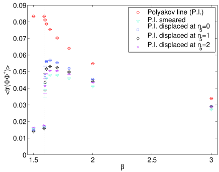
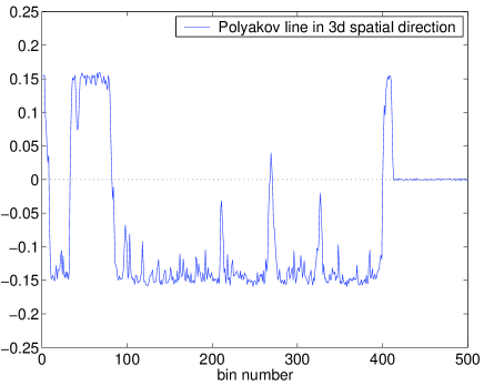
Figure 5: The phase transition on the orbifold at $N_{5}=4$. The plot on the left hand side shows the behaviour of vacuum expectations values $\langle{\rm tr}\{\Phi^{\dagger}\Phi\}\rangle$ for different Higgs fields. The plot on the right hand side shows a metastability in the Polyakov line in one of the three-dimensional directions right at the phase transition $\beta_{c}=1.5975$.

In infinite volume or with periodic boundary conditions on a finite torus five-dimensional $SU(N)$ gauge theories have at least two phases [?,?,?], a confinement massive phase at small values of $\beta$ and a deconfinement or Coulomb massless phase at large values of $\beta$. For $SU(2)$ the phase transition is located at $\beta_{c}=1.64$ [?,?]. With orbifold boundary conditions this phase transition persists but the critical value $\beta_{c}$ depends on $N_{5}$ and on $L/a$. It is signalled by a jump in the expectation values of plaquettes, see [?]. In Fig. 5 the plot on the left hand side shows what happens on the orbifold with $N_{5}=4$ and $L/a=8$ with vacuum expectation values ${\rm tr}\{\Phi\Phi^{\dagger}\}$, where for $\Phi$ we take some of the Higgs fields as explained in the legend and in Section 3. There is a clear discontinuity in the vacuum expectation values at $\beta_{c}=1.5975$.

There is a strong indication that the phase transition is of first order. The plot on the right hand side of Fig. 5 shows the history of the expectation value of the Polyakov line in one of the three-dimensional space directions evaluated at the boundary $n_{5}=0$ of the orbifold. As it was shown in early Monte Carlo study of $SU(2)$ gauge theory at finite temperature [?,?] the expectation value of the Polyakov line is zero in the confined phase and it becomes nonzero in the deconfinement phase, thereby breaking spontaneously a $\mathbb{Z}_{2}$ symmetry which changed the sign of the Polyakov line. In finite volume one actually observes in the Monte Carlo history jumps between the $\mathbb{Z}_{2}$ states. Precisely both of these behaviours can be seen on the right hand side of Fig. 5. Until about bin number 400 the system was in the deconfined phase and then it changes into the confined phase.

The location of the phase transition depends not only on $N_{5}$ but also on the ratio $L/a/N_{5}$. In principle we would like to be in a situation where $N_{5}\ll L/a$ in order to have a compact extra dimension. But the meaning of compactification will have to be qualified by looking at the results for the particle spectrum.

4.2 Higgs and photon spectra

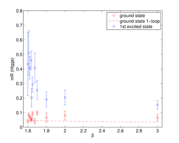
Figure 6: The ground and first excited state of the Higgs. Scan in $\beta$ at fixed $N_{5}=4$. Masses are in units of $1/R$. The dashed line represents the 1-loop result for the ground state.

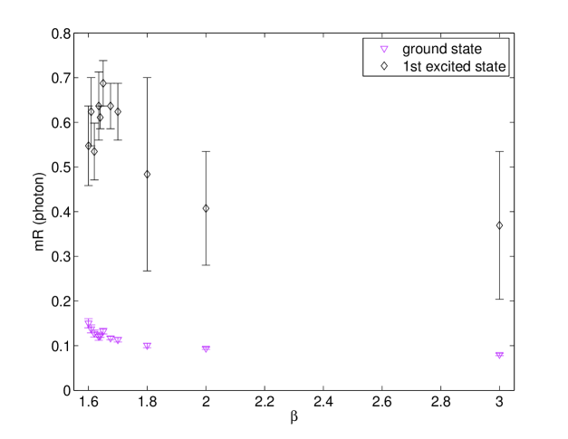
Figure 7: The ground and first excited state of the photon. Scan in $\beta$ at fixed $N_{5}=4$. Masses are in units of $1/R$.

In Fig. 6 and Fig. 7 the Higgs and photon masses for the ground state and the first excited state are shown as a function of $\beta$ in units of $1/R$ for the $N_{5}=4$, $L/a=8$ and $T/a=96$ orbifold geometry. It was not possible to extract these masses for $\beta<\beta_{c}=1.5975$. In the confined phase the signal for the effective masses disappears immediately in noise. Right above the phase transition the signal for the particle masses is there.

The first observation, looking at Fig. 6, concerns the Higgs ground state mass $m_{h}$. For all $\beta>\beta_{c}$ the Higgs mass is consistent with its value computed in 1-loop perturbation theory: for general gauge group $G=SU(N)$ this is

$$m_{h}R = \frac{c}{\sqrt{N_{5}\beta}}\,,$$ (4.55)

where $c=3/(4\pi^{2})\sqrt{N\zeta(3)C_{2}(G)/2}$ and $C_{2}(G)=N$ ($c=0.1178$ for $SU(2)$). Here we have taken the continuum result in [?] and replaced the dimensionful coupling $g_{5}$ by its lattice definition Eq. (2.3).

The second observation, looking at Fig. 7, concerns the photon ground state mass $m_{\gamma}$. Contrary to the 1-loop prediction [?] the photon mass is non-zero for all $\beta>\beta_{c}$. The photon mass even increases as the phase transition is approached. This means that there is spontaneous symmetry breaking in the pure gauge theory. This is, to our best knowledge, the first non-perturbative evidence for the Higgs mechanism originating from an extra dimension.

The third observation, looking at both Fig. 6 and Fig. 7, concerns the excited state masses for the Higgs $m_{h}^{\star}$ and the photon $m_{\gamma}^{*}$. In perturbation theory, the first excited (Kaluza–Klein) states are expected to appear split from the ground states by $(\Delta m)R=1$, the second with a mass splitting twice that, and so forth. In no range of $\beta$ we see excited states at about 1 in units of $1/R$. Close to the phase transition the excited states are separated from the ground state, especially in the case of the photon. Instead for larger $\beta$ they get closer in mass to the ground states. This is an indication that at fixed $N_{5}=4$ the system behaves more like a compact system close to the phase transition rather than for large $\beta$.

$\beta$	$L/a$	$m_{h}R$	$m_{\gamma}R$	$m_{\gamma}^{*}R$
1.609	8	0.085(13)	0.138(9)	0.62(8)
1.609	12	0.075(10)	0.202(20)	0.48(8)
1.65	8	0.093(14)	0.132(6)	0.69(5)
1.65	12	0.120(14)	0.120(13)	0.61(5)
1.80	8	0.052(24)	0.079(4)	0.38(17)
1.80	12	0.048(13)	0.097(5)	0.70(6)

Table 1: Finite volume study of the spectrum at $N_{5}=4$. The excited state of the Higgs could not be determined at $L/a=12$.

At this point one might worry about finite $L$ effects in the particle masses. Especially so for the photon mass, since its non-zero value contradicts perturbation theory. In Table 1 we offer a comparison at several $\beta$ values of the particle masses between $L/a=8$ and $L/a=12$. One can see that finite $L$ effects are small and in most cases not significant. For sure there is no variation that could be explained with a behaviour $m\propto 1/L$ which is characteristic of finite volume effects.

4.3 Static potential in the four-dimensional slices

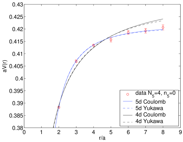
Figure 8: The static potential at $\beta=1.609$ and $N_{5}=4$ between static charges on the boundary. The five-dimensional fits are clearly favoured.

In this section we present simulation data for the static potential in the boundary slice, see Section 3.3, together with the results of various fits. Since we know from the results in Section 4.2 that the gauge boson associated with the $U(1)$ gauge symmetry on the boundary is massive, the physically motivated fits are Yukawa potentials

$$aV(r) = -c_{1}\exp(-m_{\gamma}r)/(r/a)+c_{0}\qquad\mbox{in four dimensions}\,,$$ (4.56)

$$aV(r) = -d_{1}K_{1}(m_{\gamma}r)/(r/a)+d_{0}\qquad\mbox{in five dimensions}\,,$$ (4.57)

where $c_{0},c_{1}$ and $d_{0},d_{1}$ are the fit parameters and the photon mass $m_{\gamma}$ is the one measured in the simulations. In Appendix B we derive the five-dimensional form of Yukawa potentials. It is interesting to compare the Yukawa fits with Coulomb fits

$$aV(r) = -f_{1}/(r/a)+f_{0}\qquad\mbox{in four dimensions}\,,$$ (4.58)

$$aV(r) = -e_{1}/(r/a)^{2}+e_{0}\qquad\mbox{in five dimensions}\,,$$ (4.59)

where $f_{0},f_{1}$ and $e_{0},e_{1}$ are the fits parameters.

$N_{5}$	5d Coulomb	5d Yukawa	4d Coulomb	4d Yukawa
4	0.4	0.6	14	10
6	1.1	1.9	4.2	1.7

Table 2: The values of $\chi^{2}$/(degrees of freedom) for the various fits to the static potential at the boundary at $\beta=1.609$. A comparison between $N_{5}=4$ and $N_{5}=6$ is made.

In Fig. 8 we present results from a simulation of the orbifold geometry $T/a=32$, $L/a=16$ and $N_{5}=4$. The statistics is of 20’000 measurements of the potential. The photon mass is $am_{\gamma}=0.108(7)$ (for the fits we neglect its error), measured in the simulations described in Section 4.2. In the fits only the points $r/a=2,\ldots,8$ are included. The $\chi^{2}$ per degree of freedom are listed in Table 2. The four-dimensional fits are excluded whereas the five-dimensional ones are very good.

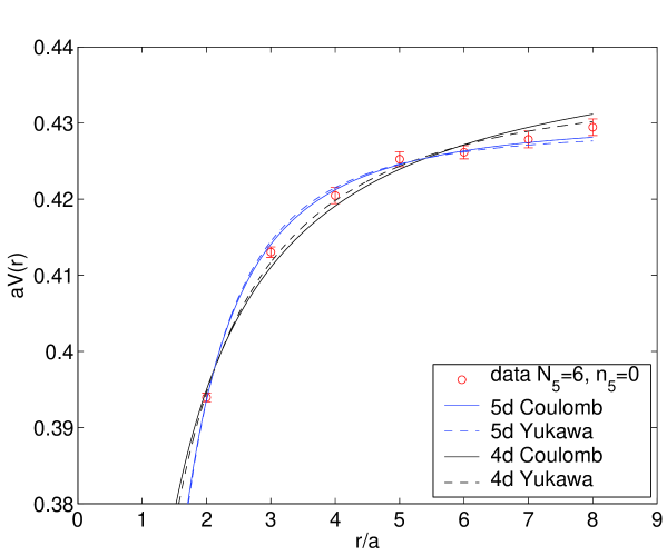
Figure 9: The static potential at $\beta=1.609$ and $N_{5}=6$ between static charges on the boundary. Besides the five-dimensional fits also a four-dimensional Yukawa fit can describe the data.

The data at $N_{5}=4$ might suffer from the fact that the ratio between the cut-off and the compactification scale is only $R/a=N_{5}/\pi\simeq 1.3$. In Fig. 9 we present results from a simulation of the orbifold geometry $T/a=32$, $L/a=16$ and $N_{5}=6$. The statistics is of 9’000 measurements of the potential. The photon mass is $am_{\gamma}=0.173(18)$, taken from a simulation at the same $\beta$ and $N_{5}$ values but with $T/a=96$ and $L/a=12$. In Table 2 we can compare the $\chi^{2}$ per degree of freedom. We see that at $N_{5}=6$ together with the five-dimensional fits also the four-dimensional Yukawa form is a good fit. The four-dimensional Coulomb fit is instead excluded. It should be noted that the errors on the potential data are comparable at both values of $N_{5}$.

We also measured the static potential in the middle slice at $n_{5}=2$. The results of the fits confirm the conclusions from the fits in the boundary slice at $N_{5}=4$, that is the four-dimensional forms are disfavoured. The $\chi^{2}$ values are now about 3 for the four-dimensional forms and 0.3 for the five-dimensional forms. At $N_{5}=6$ the statistical errors are too large and all the fits are equally good. As was discussed in Section 3.3 we have to improve the measurements of the static potential, especially for the middle slice. It is important to have precise data for the latter, since any difference with respect to the potential on the boundary might be a hint of localization effects.

4.4 Discussion

A certainly surprising feature of these models emerges when we look at the mass spectrum itself, measured in $R$-units. We have seen in Fig. 6 that when the compactification scale is lower than the cut-off scale by a fixed gap (i.e. for $N_{5}$ fixed), the Higgs ground state mass is consistent with its 1-loop perturbative value not only at large values of $\beta$ but also in the definitely non-perturbative region when $\beta$ is close to its critical value at the phase transition. Moreover also the photon mass has a mild dependence on $\beta$, see Fig. 7. Since we do not have at present any powerful analytical tools to explain these observations, we will keep our discussion at a qualitative level.

We would like to argue that one way to interpret this peculiar phenomenon is by a very mild cut-off dependence of the five-dimensional bare coupling $g_{5}^{2}$ in the non-perturbative regime. The generic situation observed in our simulations, as far as the spectrum is concerned, can be translated in an effective field theory language by saying that the theory possesses a region in its parameter space such that any operator of dimension $5+p$ appearing in the effective action and effective operators scales as

$$\frac{{\cal Z}(g_{0},g_{4})}{\Lambda^{p}}{\cal O}^{(5+p)}\,,$$ (4.60)

with ${\cal Z}(g_{0},g_{4})$ a very slowly varying function of the dimensionless bare couplings $g_{0}=g_{5}\sqrt{\Lambda}$ and $g_{4}=g_{5}/\sqrt{\pi R}$, at least as long as the ratio $\Lambda/(1/R)$ is kept fixed. In the orbifold theory, taking the Higgs mass as an example, we recall that a boundary counterterm is non-perturbatively excluded and thus all possible corrections come from either pure bulk effects or bulk effects with boundary insertions, both of which descend directly from the circle.

In an attempt to predict the explicit cut-off dependence in Eq. (4.60), we note that naive dimensional analysis tells us that as $\beta$ decreases with $g_{5}$ fixed, the cut-off increases, see Eq. (2.3). The compactification scale is $1/R$ and a wide separation from the cut-off scale requires $\Lambda>>1/R$. Increasing $\beta$ while keeping the gap between the compactification and cut-off scales fixed, would require decreasing $\Lambda$ (at fixed $g_{5}$) and therefore an increase of $R$, which drives the fifth dimension to its decompactification limit. A general lesson then is that for fixed $N_{5}$, moving towards the large $\beta$ regime is expected to enhance the cut-off effects (appearing as $E/\Lambda$ at low energies $E$ in the sense of an effective action) and decompactify the theory, whereas moving in the opposite direction, i.e. towards smaller $\beta$, is expected to suppress the cut-off effects and drive the system into a compactified but non-perturbative regime. Eventually the phase transition is reached at the critical value of $\beta=\beta_{c}$, where the cut-off reaches its maximal value. There is a possible caveat though in this argument: we have implicitly assumed that it makes sense to vary the cut-off while keeping the dimensionful coupling $g_{5}$ fixed for all values $\beta_{c}<\beta<\infty$.

If we look at the spectrum of the excited states of the Higgs and the photon in Fig. 6 and Fig. 7, we see that as $\beta$ grows their masses decrease, thus deviating more and more from their expected perturbative value as Kaluza–Klein states of mass $\simeq 1/R$. This fact could be explained with our argument that cut-off effects increase at large $\beta$. We cannot at the moment explain why these cut-off effects would affect the excited states but not the ground states.

Next, let us see what happens when we start changing $N_{5}$ while keeping $\beta$ fixed. The cut-off $\Lambda$ depends only on $\beta$ and is also fixed. Using Eq. (2.2) we obtain that

$$\frac{\delta N_{5}}{N_{5}}=\frac{\delta R}{R}$$ (4.61)

which implies that increasing $N_{5}$ amounts to increasing also $R$. Thus, in a compactified scenario we expect to be able to approach an effective dimensional reduction by decreasing $N_{5}$. It is interesting to note that according to our potential data we observe an opposite effect: the fit to a four dimensional Yukawa law becomes much better when we increase $N_{5}$ from 4 to 6 at fixed $\beta$, namely when we decompactify the extra dimension. Therefore, to the extent that this result can be considered as a firm physical property of the system in this region of the parameter space, we are lead to the conclusion that the fact that we start observing an effective dimensional reduction at $N_{5}=6$ is more likely to be a consequence of a localization mechanism rather than an effect of compactification. It is possible that the region that corresponds to dimensional reduction from compactification is located at much smaller $N_{5}$ which would however require an anisotropic lattice to be probed.

Finally, regarding the applicability of the vicinity of the phase transition in model building, we would like to point out that even though it clearly corresponds to a strong coupling regime from the point of view of five dimensions, viewed from the point of view of the four-dimensional effective theory with an effective coupling defined as in Eq. (2.4), it could correspond to a weakly coupled regime, if for example large renormalization factors change Eq. (2.4).

5 Conclusions

The first results for the spectrum of the orbifold theory simulated on a lattice with an extra dimension of the size of $N_{5}=4$ lattice spacings, show that there is spontaneous symmetry breaking, which manifests in a massive gauge boson associated with the $U(1)$ boundary gauge group. This result was unexpected from computations at 1-loop in perturbation theory, where the photon remains massless. Moreover, the Higgs mass is also measured in a large range of gauge coupling and it is always close to its perturbative value. The excited state masses for the Higgs and the photon are not at the scale of the inverse compactification radius, where they are expected to be in a scenario of dimensional reduction like in finite temperature field theory. But close to the orbifold phase transition the mass splitting between the ground states and the first excited states increases. Data for the static potential strongly suggest five-dimensional potential forms, both when the static potential is measured with the charges on the boundary slice or in the middle slice along the extra dimension. We have also presented potential data at $N_{5}=6$. They indicate that a four-dimensional Yukawa form, with the vector boson mass equal to the measured photon mass, is a good fit to the potential on the boundary together with the five-dimensional forms.

The results we have so far give a consistent picture and they motivate for further work to explore the phase diagram of the orbifold theory. Despite its non-renormalizability, the theory makes finite predictions for the mass spectrum and we would like to understand better how to change the lattice parameters to study the scaling properties. This also requires technical improvements, for the basis of Higgs operators and for the static potential.

Acknowledgement. We thank B. Bunk for his help in the construction of the programming code. We are grateful to P. de Forcrand, M. Della Morte, P. Hasenfratz, Y. Hosotani, M. Lüscher and U.-J. Wiese for discussions and helpful suggestions. We thank the Swiss National Supercomputing Centre (CSCS) in Manno (Switzerland) for allocating computer resources to this project. N. Irges thanks CERN for hospitality.

Appendix A Higgs potential from extra dimension(s)

In this Appendix we review the calculation of 1-loop potentials in orbifold gauge theories. This material is already well known in the hep-ph community but since it is perhaps less familiar in the lattice community, for completeness we reproduce here in detail the perturbative arguments for the existence or not of spontaneous symmetry breaking, reproducing essentially some of the the results of [?].

Consider a (massive) free field theory for a one–component real scalar field in D-dimensions with action $S$. After a Euclidean rotation, the path intergral that defines the vacuum energy $\Gamma$ is [?]:

$${\rm e}^{-\Gamma}=\int[D\phi]\;e^{-S_{E}}\sim\frac{1}{\sqrt{\det{[\Box+M^{2}]}}}\,,\quad\Box=-\partial_{\mu}\partial_{\mu}\,.$$ (A.62)

The mass (M) dependence of the above can be extracted by using the identity

$$\log\left(\det A\right)=-\int_{\epsilon}^{\infty}\frac{{\rm d}t}{t}{\rm tr}\left({\rm e}^{-tA}\right).$$ (A.63)

We obtain

$$\Gamma=-\log\left[\frac{1}{\sqrt{\det{[\Box+M^{2}]}}}\right]=-\frac{1}{2}\frac{\pi^{D/2}}{(2\pi)^{D}}\int_{0}^{\infty}\frac{{\rm d}t}{t^{\frac{D+2}{2}}}{\rm e}^{-tM^{2}}$$ (A.64)

For a fermionic free field we have

$${\rm e}^{-\Gamma}=\det(D)\,,\quad D=\gamma_{\mu}\partial_{\mu}+M\,.$$ (A.65)

The nonzero eigenvalues of the Dirac operator come in complex conjugate pairs $\pm i\alpha+M$, hence

$$\det(D)=\sqrt{\det(DD^{\dagger})}=\sqrt{\det[\Box+M^{2}]}\,.$$ (A.66)

We can therefore summarize the contributions to the effective action, setting $D=4$, as

$$\Gamma = -\frac{1}{32\pi^{2}}\sum_{I}(-)^{F_{I}}\int_{0}^{\infty}{\rm d}l\;l\;{\rm e}^{-\frac{M_{I}^{2}}{l}}\,,$$ (A.67)

where $F_{I}$ is 0 for bosonic and 1 for fermionic degrees of freedom of mass $M_{I}$.

Let us apply the above for the case where there are $d$ extra compact toroidal directions. For the four-dimensional theory, after dimensional reduction, i.e. Kaluza–Klein decomposition, we obtain the mass formula

$$M^{2}_{I}=m^{2}_{I}+\sum_{i=1}^{d}\left(\frac{n_{i}+a_{i}^{I}}{R_{i}}\right)^{2},$$ (A.68)

where

• $R_{i}$ are the radii of the $d$ circles of the torus.

• $\{n_{i}\},\;i=1,\ldots,d$ are integers.

• $m^{2}_{I}$ is a $4+d$-dimensional mass which remains in the $R_{i}\longrightarrow\infty$ limit. This is zero for a pure gauge theory.

• The shifts $a_{i}^{I}$ originate from the possible failure for periodicity of the $4+d$ dimensional field $\Phi_{I}$:

  $$\Phi_{I}(x^{\mu},y^{i}+2\pi k_{i}R_{i})=e^{2i\pi\sum_{i}k_{i}a_{i}^{I}}\Phi_{I}(x^{\mu},y^{i}),$$ (A.69)

  where $y_{i}$ are the coordinates of the circles.

According to the above, for the $T^{d}$ torus we have the expression for the potential

$$V_{eff}^{T^{d}}=-\sum_{I}\sum_{\{n_{i}\}}(-)^{F_{I}}\frac{1}{32\pi^{2}}\int_{0}^{\infty}{\rm d}l\,l\,e^{-\sum_{i}\frac{(n_{i}+a_{i}^{I})^{2}}{R_{i}^{2}l}}.$$ (A.70)

By commuting the integral with the sum over $n_{i}$ and then performing a Poisson resummation using the formula

$$\sum_{\{n_{i}\}}e^{{-\pi\;{\bf n}^{T}{\bf A}{\bf n}}+2i\pi{\bf b}^{T}{\bf n}}=\frac{1}{\sqrt{\det{\bf A}}}\sum_{\{m_{i}\}}e^{-\pi\;({\bf m-b})^{T}{\bf A}^{-1}({\bf m-b})}$$ (A.71)

where ${\bf A}$ is a $d\times d$ (invertible) matrix and ${\bf n}$ and ${\bf m}$ are $d$ dimensional KK number vectors, we find

$$V_{eff}^{T^{d}}=-\sum_{I}(-)^{F_{I}}\frac{\left(\prod_{i}R_{i}\right)}{32\pi^{\frac{4-d}{2}}}\sum_{\{n_{i}\}}{\rm e}^{2i\pi\sum_{i}n_{i}a_{i}^{I}}\int_{0}^{\infty}{\rm d}l\,l^{\frac{2+d}{2}}\,e^{-\pi^{2}l\sum_{i}n_{i}^{2}R_{i}^{2}}.$$ (A.72)

The terms with $n_{i}=0$ give rise to a divergent contribution to the vacum energy. They represent a contribution to the cosmological constant and can be neglected for the present discussion. For all other non-vanishing vectors $\vec{n}$ we perform the integral explicitly. This leads to the finite result

$$V_{eff}^{T^{d}}=-\sum_{I}(-)^{F_{I}}\frac{\Gamma\left(\frac{4+d}{2}\right)}{32\pi^{\frac{12+d}{2}}}\left(\prod_{i}R_{i}\right)\sum_{\vec{n}\neq 0}\frac{e^{2\pi i\sum_{i}n_{i}a_{i}^{I}}}{\left(\sum_{i}n_{i}^{2}R_{i}^{2}\right)^{\frac{4+d}{2}}}.$$ (A.73)

A.1 5D $SU(2)$ gauge theory on $S^{1}/Z_{2}$

For a 5D theory compactified on the 1 dimensional torus, the circle, we have $d=1$. Then

$$V_{eff}^{S^{1}}=-\sum_{I}(-)^{F_{I}}\frac{\Gamma\left(\frac{5}{2}\right)}{32\pi^{\frac{13}{2}}}\,R\,\sum_{n\neq 0}\frac{e^{2\pi ina^{I}}}{\left(n^{2}R^{2}\right)^{\frac{5}{2}}}=-\frac{3}{64\pi^{6}R^{4}}\sum_{I}(-)^{F_{I}}\left[\sum_{n=1}^{\infty}\frac{\cos{(2\pi na^{I})}}{n^{5}}\right].$$ (A.74)

For a pure gauge theory we have in addition that $F_{I}=0$. We then finally obtain for the vacuum energy

$$V_{eff}^{S^{1}}=-\frac{3}{64\pi^{6}R^{4}}\sum_{A}\sum_{n=1}^{\infty}\frac{\cos{(2\pi na^{A})}}{n^{5}}$$ (A.75)

where the index $I$ has been changed to $A$, indicating the adjoint representation of some gauge group. This potential may have a minimum that leads to an extra dimensional version of the Higgs mechanism.

There are different cases where a failure of periodicity can happen and a shift in the KK formula is generated. One particularly interesting example is the presence of a Wilson line in an extra dimensional gauge theory

$$a^{A}=q^{A}\,g_{5}\,\int_{S^{1}}\frac{dy}{2\pi}\,A_{5}^{A},$$ (A.76)

where $A_{5}^{A}$ is the internal component of the gauge field with gauge coupling $g_{5}$ and $q_{A}$ the charge of the $A$th field under the corresponding generator. To be more concrete, let us look at an example. Consider a 5D $SU(2)$ gauge theory compactified on the circle. In order to compute the vacuum energy, according to eq. (A.75) the only quantity we need to compute are the $a^{A}$. To compute the $a^{A}$ we have to compute the eigenvalues of the mass-squared operator [?]

$$-D_{M}D_{M}=-D_{\mu}D_{\mu}-D_{5}D_{5}\quad\mbox{(in Euclidean space)}$$ (A.77)

in the vacuum, with $D_{M}$ acting on fields $F=F^{A}T^{A}$ in the adjoint representation as

$$D_{M}F = \partial_{M}F+[B_{M},F]\,,\quad B_{M}=\langle A_{M}\rangle\,.$$ (A.78)

$B_{M}$ is a constant background field given by the vacuum expectation value (vev) of $A_{M}$.

After orbifolding, which breaks $SU(2)\longrightarrow U(1)$ the only fields that can take a vev are $A_{5}^{1}(x^{5})$ and $A_{5}^{2}(x^{5})$. The unbroken $U(1)$ invariance can be used to rotate the vev’s in such a way that we have

$$B_{5}^{1}=H\,,\quad B_{5}^{2}=B_{5}^{3}=0\,,\quad B_{5}=-ig_{5}B_{5}^{A}T^{A}\,.$$ (A.79)

The non-trivial part comes from the $D_{5}D_{5}$ part of the operator acting on $x^{5}$ dependent parts of the gauge fields. Writing out this explicitly in the vacuum acting on an adjoint field $F$,

$$D_{5}D_{5}F = \partial_{5}\partial_{5}F+2[B_{5},\partial_{5}F]+[B_{5},[B_{5},F]]\,,$$ (A.80)

gives the operator

$$\left(D_{5}D_{5}\right)_{AB}=\pmatrix{\partial_{5}\partial_{5}&0&0\cr 0&\partial_{5}\partial_{5}-g_{5}^{2}HH&-2g_{5}H\partial_{5}\cr 0&2g_{5}H\partial_{5}&\partial_{5}\partial_{5}-g_{5}^{2}HH}.$$ (A.81)

Since this operator does not mix different KK modes we can diagonalize it separately for each level $n$.

• Eigenvalues of $A_{\mu}^{A}$.

  The matrix elements of the $-D_{5}D^{5}$ operator

  $$\langle f|-D_{5}D_{5}|g\rangle = \int_{0}^{2\pi R}{\rm d}x^{5}\,f^{*}(x^{5})(-D_{5}D_{5})g(x^{5})$$ (A.82)

  can be easily obtained by using the basis of orthonormal functions

  $$\frac{1}{\sqrt{\pi R}}\cos{\frac{n}{R}x^{5}},\hskip 14.22636pt{\rm for}\;A,B=3$$ (A.83)

  since $A_{\mu}^{3}$ is even under the orbifold, and

  $$\frac{1}{\sqrt{\pi R}}\sin{\frac{n}{R}x^{5}},\hskip 14.22636pt{\rm for}\;A,B=1,2$$ (A.84)

  since $A_{\mu}^{1,2}$ are odd under the orbifold. The matrix we obtain for $n\neq 0$ is

  $$A_{\mu}^{A\,(n\neq 0)}\longrightarrow\pmatrix{\frac{n^{2}}{R^{2}}&0&0\cr 0&\frac{n^{2}}{R^{2}}+\frac{\alpha^{2}}{R^{2}}&-2\frac{\alpha n}{R^{2}}\cr 0&-2\frac{\alpha n}{R^{2}}&\frac{n^{2}}{R^{2}}+\frac{\alpha^{2}}{R^{2}}}\longrightarrow\frac{n^{2}}{R^{2}},\frac{(|n|+\alpha)^{2}}{R^{2}},\frac{(|n|-\alpha)^{2}}{R^{2}}\,,$$ (A.85)

  where

  $$\alpha=g_{5}\,H\,R$$ (A.86)

  and on the right we have given the eigenvalues. For $n=0$, the $A_{\mu}^{1,2}$ do not have zero modes but $A_{\mu}^{3}$ does have a zero mode whose eigenvalue is

  $$A_{\mu}^{3,(0)}\longrightarrow\frac{\alpha^{2}}{R^{2}}.$$ (A.87)

• Eigenvalues of ghosts.

  We notice that the ghosts have the same $Z_{2}$ parity assignement as the gauge fields $A_{\mu}$ therefore the effect of the ghosts is to just reduce the degree of polarization as $4\rightarrow 2$.

• Eigenvalues of $A_{5}^{A}$.

  Since the $Z_{2}$ parities of the $A_{5}^{A}$ are the opposite from those of $A_{\mu}^{A}$, we will obtain

  $$A_{\mu}^{1,2,(0)}\longrightarrow\frac{\alpha^{2}}{R^{2}}$$ (A.88)

  and

  $$A_{5}^{A\,(n\neq 0)}\longrightarrow\frac{n^{2}}{R^{2}},\frac{(|n|+\alpha)^{2}}{R^{2}},\frac{(|n|-\alpha)^{2}}{R^{2}}\,.$$ (A.89)

By comparing with Eq. (A.68) we see that non-zero shifts $a^{I}$ are given by $\pm\alpha$ in Eq. (A.85) and Eq. (A.89). As we have argued, only the non-zero modes are relevant for the vacuum energy. We count $2+1$ (2 from physical degrees of polarization of $A_{\mu}$, 1 from $A_{5}$) eigenvalues $(n+\alpha)^{2}/R^{2}$ (with $a^{I}=\alpha$) and an equal number of eigenvalues $(n-\alpha)^{2}/R^{2}$ (with $a^{I}=-\alpha$). Furthermore, as can be seen from eq. (A.75) the $a^{I}=-\alpha$ contribution is the same as the $a^{I}=+\alpha$ contribution. We then obtain for the vacum energy the final result

$$V_{eff}^{S^{1}}(SU(2))=-\frac{3\cdot 3\cdot 2}{64\pi^{6}R^{4}}\sum_{n=1}^{\infty}\frac{\cos{(2\pi n\alpha)}}{n^{5}}\,.$$ (A.90)

This potential could, in principle break the remaining $U(1)$ down to nothing on the branes. Plotting the potential one can see that it has two degenerate minima at $\alpha=0$ and $\alpha=1$, none of which breaks $U(1)$.

A similar computation gives for the $SU(3)\longrightarrow SU(2)\times U(1)$ model the potential

$$V_{eff}^{S^{1}}(SU(3))=-\frac{3\cdot 3\cdot 2}{64\pi^{6}R^{4}}\sum_{n=1}^{\infty}\frac{1}{n^{5}}\left[\cos{(2\pi n\alpha)}+2\cos{(\pi n\alpha)}\right].$$ (A.91)

The latter can be seen by noticing that the eigenvalues for the adjoint of $SU(3)$ are

$$2\times\frac{n^{2}}{R^{2}},\hskip 14.22636pt\frac{(n\pm\alpha)^{2}}{R^{2}}\hskip 14.22636pt2\times\frac{(n\pm\frac{\alpha}{2})^{2}}{R^{2}}.$$ (A.92)

Again, the minimum is at $\alpha=0$ which does not break $SU(2)\times U(1)$.

In fact, in some cases a useful criterion to see if it is possible to break the symmetry by the Hosotani mechanism is to use the statement proven in [?]: The Hosotani mechanism does not reduce the rank of ${\cal H}$ if the symmetry breaking global minimum is at $\alpha=1$. To show this statement, we can compute the Wilson line due to the vev $H=\frac{1}{g_{5}R}$ of a scalar along the $T^{A}$ direction:

$$\langle W\rangle={\mathcal{P}}{\rm e}^{-ig_{5}\oint{\rm d}x^{5}\,H\,T^{A}}={\rm e}^{-2\pi iT^{A}}\,.$$ (A.93)

It is straightforward to show that $\exp(-2\pi iT^{A})$ is a diagonal matrix. In the case of $SU(2)$: $\exp(-i\pi\sigma_{1})=-\mathbf{1}_{2}=\exp(-i\pi\sigma_{2})$. For $SU(N)$, the non-diagonal generators are obtained embedding $\sigma_{1,2}$. Thus, we always have that

$$[\langle W\rangle,H_{i}]=0,$$ (A.94)

where $H_{i}$ are the generators corresponding to the Cartan subalgebra of ${\cal G}$, i.e. that the Wilson loop commutes with at least those generators and therefore it leaves at least a $U(1)_{1}\times\cdots\times U(1)_{rank({\cal H})}$ unbroken. From this it is clear that in the $SU(2)$ model, $U(1)$ can not break further with $\alpha=1$. For the $SU(3)$ model $\alpha=1$ could break $SU(2)\times U(1)$ down to $U(1)\times U(1)$ by the Hosotani mechanism. In both cases, it is not clear what $\alpha\neq 1$ would do.

Appendix B The Yukawa potential in 5D

The potential is given by the integral

$$V(x)=\int\frac{d^{4}q}{(2\pi)^{4}}\frac{e^{iq\cdot x}}{q^{2}+m^{2}}$$ (B.95)

where $|x|=r$, $q=|q|q^{\prime}$, $|q^{\prime}|=1$ and

$$q_{1}^{\prime}=\cos{\phi_{1}}$$

$$q_{2}^{\prime}=\sin{\phi_{1}}\cos{\phi_{2}}$$

$$q_{3}^{\prime}=\sin{\phi_{1}}\sin{\phi_{2}}\cos{\theta}$$

$$q_{4}^{\prime}=\sin{\phi_{1}}\sin{\phi_{2}}\sin{\theta}$$ (B.96)

where $0\leq\phi_{j}\leq\pi,0\leq\theta\leq 2\pi$. Then the potential can be written as

$$V(x)=\frac{1}{(2\pi)^{4}}\int_{0}^{\infty}d|q||q|^{3}\int_{0}^{2\pi}d\theta\int_{0}^{\pi}d\phi_{1}\int_{0}^{\pi}d\phi_{2}\sin^{2}\phi_{1}\sin\phi_{2}\frac{e^{iq\cdot x}}{q^{2}+m^{2}}.$$ (B.97)

Choosing coordinates such that $x=r\cdot e_{1}$ with $e_{1}$ a unit vector, we have that $q\cdot x=|q|r\cos\phi_{1}$ and then

$$V(x)=\frac{1}{(2\pi)^{4}}\int_{0}^{\infty}d|q|\frac{|q|^{3}}{|q|^{2}+m^{2}}\int_{0}^{2\pi}d\theta\int_{0}^{\pi}d\phi_{2}\sin\phi_{2}\int_{0}^{\pi}d\phi_{1}\sin^{2}\phi_{1}e^{i|q|r\cos\phi_{1}}.$$ (B.98)

Performing the angular integrals we obtain

$$V(x)=\frac{1}{(2\pi)^{2}}\frac{1}{r}\int_{0}^{\infty}d|q|\frac{|q|^{2}}{|q|^{2}+m^{2}}J_{1}(|q|r).$$ (B.99)

Finally, changing variables as $y=|q|r$ one has the left over radial integral

$$V(x)=\frac{1}{(2\pi)^{2}r^{2}}\int_{0}^{\infty}dy\frac{y^{2}}{y^{2}+(mr)^{2}}J_{1}(y),$$ (B.100)

which can be done, yielding the result

$$V(x)\sim\frac{1}{(2\pi)^{2}r^{2}}(mr)K_{1}(mr).$$ (B.101)

As $r\longrightarrow 0$, the Bessel function $(mr)K_{1}(mr)\longrightarrow 1$ so we have at short distances

$$r\longrightarrow 0:\hskip 28.45274ptV(x)=\frac{1}{(2\pi)^{2}r^{2}}.$$ (B.102)

For large $r$ on the other hand we have

$$r\longrightarrow\infty:\hskip 28.45274ptV(x)=\sqrt{\frac{{\pi m}}{2}}\frac{1}{(2\pi)^{2}}\frac{e^{-mr}}{r^{3/2}}.$$ (B.103)

References

- [1] S.R. Coleman and E. Weinberg, Phys. Rev. D7 (1973) 1888.
- [2] D.B. Fairlie, Phys. Lett. B82 (1979) 97.
- [3] D.B. Fairlie, J. Phys. G5 (1979) L55.
- [4] N.S. Manton, Nucl. Phys. B158 (1979) 141.
- [5] P. Forgacs and N.S. Manton, Commun. Math. Phys. 72 (1980) 15.
- [6] Y. Hosotani, Phys. Lett. B126 (1983) 309.
- [7] Y. Hosotani, Ann. Phys. 190 (1989) 233.
- [8] I. Antoniadis, K. Benakli and M. Quiros, New J. Phys. 3 (2001) 20, hep-th/0108005.
- [9] G.R. Dvali, S. Randjbar-Daemi and R. Tabbash, Phys. Rev. D65 (2002) 064021, hep-ph/0102307.
- [10] N. Arkani-Hamed, A.G. Cohen and H. Georgi, Phys. Lett. B513 (2001) 232, hep-ph/0105239.
- [11] G. von Gersdorff, N. Irges and M. Quiros, Nucl. Phys. B635 (2002) 127, hep-th/0204223.
- [12] H.C. Cheng, K.T. Matchev and M. Schmaltz, Phys. Rev. D66 (2002) 036005, hep-ph/0204342.
- [13] N. Arkani-Hamed, L.J. Hall, Y. Nomura, D.R. Smith and N. Weiner, Nucl. Phys. B605 (2001) 81, hep-ph/0102090.
- [14] A. Masiero, C.A. Scrucca, M. Serone and L. Silvestrini, Phys. Rev. Lett. 87 (2001) 251601, hep-ph/0107201.
- [15] G. von Gersdorff, N. Irges and M. Quiros, (2002), hep-ph/0206029.
- [16] G. von Gersdorff, N. Irges and M. Quiros, Phys. Lett. B551 (2003) 351, hep-ph/0210134.
- [17] N. Irges and F. Knechtli, Nucl. Phys. B719 (2005) 121, hep-lat/0411018.
- [18] G. Martinelli, M. Salvatori, C.A. Scrucca and L. Silvestrini, (2005), hep-ph/0503179.
- [19] C.S. Lim, N. Maru and K. Hasegawa, (2006), hep-th/0605180.
- [20] Y. Hosotani, (2006), hep-ph/0607064.
- [21] G. von Gersdorff and A. Hebecker, Nucl. Phys. B720 (2005) 211, hep-th/0504002.
- [22] F. Knechtli, B. Bunk and N. Irges, PoS LAT2005 (2005) 280, hep-lat/0509071.
- [23] N. Irges and F. Knechtli, (2006), hep-lat/0604006.
- [24] Y.K. Fu and H.B. Nielsen, Nucl. Phys. B236 (1984) 167.
- [25] P. Dimopoulos, K. Farakos and S. Vrentzos, (2006), hep-lat/0607033.
- [26] G.R. Dvali and M.A. Shifman, Phys. Lett. B396 (1997) 64, hep-th/9612128.
- [27] M. Laine, H.B. Meyer, K. Rummukainen and M. Shaposhnikov, JHEP 04 (2004) 027, hep-ph/0404058.
- [28] S. Chandrasekharan and U.J. Wiese, Nucl. Phys. B492 (1997) 455, hep-lat/9609042.
- [29] R. Brower, S. Chandrasekharan and U.J. Wiese, Phys. Rev. D60 (1999) 094502, hep-th/9704106.
- [30] B. Schlittgen and U.J. Wiese, Phys. Rev. D63 (2001) 085007, hep-lat/0012014.
- [31] M. Kubo, C.S. Lim and H. Yamashita, Mod. Phys. Lett. A17 (2002) 2249, hep-ph/0111327.
- [32] C.A. Scrucca, M. Serone and L. Silvestrini, Nucl. Phys. B669 (2003) 128, hep-ph/0304220.
- [33] G. Panico, M. Serone and A. Wulzer, Nucl. Phys. B739 (2006) 186, hep-ph/0510373.
- [34] J. Zinn-Justin, Quantum Field Theory and Critical Phenomena, 4th ed. (International Series of Monographs on Physics — Vol. 113, Clarendon Press, Oxford, 2002).
- [35] I. Montvay, Phys. Lett. B150 (1985) 441.
- [36] S. Ejiri, J. Kubo and M. Murata, Phys. Rev. D62 (2000) 105025, hep-ph/0006217.
- [37] G. Arnold, B. Bunk, T. Lippert and K. Schilling, Nucl. Phys. Proc. Suppl. 119 (2003) 864, hep-lat/0210010.
- [38] E.H. Fradkin and S.H. Shenker, Phys. Rev. D19 (1979) 3682.
- [39] K. Osterwalder and E. Seiler, Ann. Phys. 110 (1978) 440.
- [40] K. Jansen, J. Jersak, C.B. Lang, T. Neuhaus and G. Vones, Phys. Lett. B155 (1985) 268.
- [41] K. Symanzik, Mathematical Problems in Theoretical Physics, eds. R. Schrader et al., Lecture Notes in Physics 153 (1982) 47, Presented at 6th Int. Conf. on Mathematical Physics, Berlin, West Germany, Aug 11-21, 1981.
- [42] K. Symanzik, Nucl. Phys. B226 (1983) 187.
- [43] K. Symanzik, Nucl. Phys. B226 (1983) 205.
- [44] M. Lüscher, (1998), hep-lat/9802029.
- [45] M. Luscher and U. Wolff, Nucl. Phys. B339 (1990) 222.
- [46] I. Montvay and P. Weisz, Nucl. Phys. B290 (1987) 327.
- [47] F. Knechtli, (1999), hep-lat/9910044.
- [48] APE, M. Albanese et al., Phys. Lett. B192 (1987) 163.
- [49] M. Creutz, Phys. Rev. Lett. 43 (1979) 553.
- [50] B.B. Beard et al., Nucl. Phys. Proc. Suppl. 63 (1998) 775, hep-lat/9709120.
- [51] L.D. McLerran and B. Svetitsky, Phys. Lett. B98 (1981) 195.
- [52] J. Kuti, J. Polonyi and K. Szlachanyi, Phys. Lett. B98 (1981) 199.
- [53] K.R. Dienes, E. Dudas and T. Gherghetta, Nucl. Phys. B537 (1999) 47, hep-ph/9806292.