Exploring the infrared gluon and ghost propagators using large asymmetric lattices

Abstract

We report on the infrared limit of the quenched lattice Landau gauge gluon propagator computed from large asymmetric lattices. In particular, the compatibility of the pure power law infrared solution $(q^{2})^{2\kappa}$ of the Dyson-Schwinger equations is investigated and the exponent $\kappa$ is measured. The lattice data favours $\kappa\sim 0.52$, which would imply a vanishing zero momentum gluon propagator as predicted by the Kugo-Ojima confinement mechanism and the Zwanziger horizon condition. Results for the ghost propagator and for the running coupling constant are shown.

PACS numbers:12.38.-t; 11.15.Ha; 12.38.Gc; 12.38.Aw; 14.70.Dj; 14.80.-j

Keyword: lattice QCD; Landau gauge; confinement; gluon propagator; ghost propagator; running coupling constant.

I Introduction and motivation

The mechanism of quark and gluon confinement is not fully understood yet. The study of the fundamental Green’s functions of Quantum Chromodynamics (QCD), namely the gluon and ghost propagators, can help in the understanding of such mechanism. Indeed, there are gluon confinement criteria connected with the behaviour of the propagators at zero momentum. In particular, the Zwanziger horizon condition implies a null zero momentum gluon propagator $D(q^{2})$, and the Kugo-Ojima confinement mechanism requires an infinite zero momentum ghost propagator $G(q^{2})$. The violation of positivity for the gluon propagator can also be seen as a signal for confinement .

In QCD, the investigation of its infrared limit has to rely on non-perturbative methods like the Dyson-Schwinger equations (DSE) and lattice QCD. Both methods have good and bad features, namely we can solve analitically the DSE in the infrared, but one has to rely on a truncation of an infinite tower of equations. On the lattice, one includes all non-perturbative physics, but one has to care about finite volume and finite lattice spacing effects.

Recent studies of Dyson-Schwinger equations obtained a pure power law behaviour for the infrared gluon and ghost dressing functions,

$$Z_{gluon}(q^{2})\equiv q^{2}D(q^{2})\sim(q^{2})^{2\kappa}$$ (1)

$$Z_{ghost}(q^{2})\equiv q^{2}G(q^{2})\sim(q^{2})^{-\kappa},$$ (2)

with $\kappa=0.595$ lerche , which implies a vanishing (infinite) gluon (ghost) propagator for zero momentum. Studies using functional renormalization equations pawl ; gies provided bounds in the possible values of the infrared exponent $0.52<\kappa<0.595$. The infrared exponent obtained from time independent stochastic quantisation tisq is within these bounds ($\kappa=0.52145$).

As an infrared (IR) analytical solution of DSE, the pure power law is valid only for very low momenta. In figure 1, the DSE gluon and ghost propagators fish.penn are compared with the corresponding pure power law solution. Note that for the gluon propagator the power law is valid only for momenta below 200 MeV, and for the ghost the infrared solution is restricted to even lower momenta. If one wants to use lattice QCD to check for a pure power law behaviour, certainly one should consider a lattice volume sufficiently large to accomodate a minimum number of points in the region of interest. For symmetric lattices this would require a too large volume. A cheaper solution is the use of large asymmetric lattices $L_{s}^{3}\times L_{t}$, with $L_{t}\gg L_{s}$. For example, in sardenha ; dublin ; finvol ; nossoprd ; madrid ; tucson we use a set of asymmetric lattices with $L_{t}=256$ and $L_{s}=8,10,\ldots,18$ (see nossoprd for the technical details of the simulations). The large temporal size of these lattices allow to access to momenta as low as 48 MeV. Of course, the price to pay are finite volume effects caused by the small value of $L_{s}$.

\psfrag{EIXOX}{{\small$q(GeV)$}}\psfrag{EIXOY}{{\small$Z_{gluon}(q^{2})$}}\psfrag{GEIXY}{{\small$Z_{ghost}(q^{2})$}}\includegraphics[width=227.62204pt]{dse_powerlaw_glgh2.eps}

Figure 1: The DSE solution for the gluon and ghost dressing functions fish.penn compared with the corresponding pure power laws.

Recently, some criticism have been raised against the use of asymmetric lattices to study the infrared limit of QCD Green’s functions. In cucc06 , the authors studied the gluon and ghost propagators in SU(2) 3-d theory and reported systematic effects due to the asymmetry of the lattice, if one compares with a symmetric one. Of course, this comparison cannot be done in our case. Also in phdstern the author reported asymmetry effects in the propagators. However, in what concerns the gluon propagator, such effects have been already investigated in finvol . Furthermore, in finvol ; nossoprd it is shown that the approach $L_{s}\to+\infty$ is smooth. Indeed, a quick look at the gluon and ghost data in cucc06 , again, suggests that the approach $L_{s}\to+\infty$ is smooth, i. e. that the largest symmetric propagators can be obtained by extrapolation of the asymmetric ones. In what concerns the quantitative results coming from a single large asymmetric lattice, all the above studies show that they provide, at least, a bound on the infinite volume limit. Here we report on the status of our investigations concerning the use of asymmetric lattices to study the infrared properties of QCD. In what concerns the positivity violation of the gluon propagator, our results can be seen in tucson .

II Extracting the infrared exponent $\kappa$ from the gluon propagator

In nossoprd , we have computed the gluon propagator

$$D^{ab}_{\mu\nu}(q)=\delta^{ab}\Big{(}\delta_{\mu\nu}-\frac{q_{\mu}q_{\nu}}{q^{2}}\Big{)}D(q^{2})$$ (3)

for SU(3) four-dimensional asymmetric lattices $L_{s}^{3}\times 256$, with $L_{s}=8,10,\ldots,18$. To check that the temporal size is large enough, 164 $16^{3}\times 128$ Wilson action gauge configurations were generated. In what concerns the gluon propagator for time-like momenta, there are no differences between the $16^{3}\times 128$ and $16^{3}\times 256$ data (see figure 2). This gives us confidence that the temporal extension of our lattices is sufficiently large.

\psfrag{EIXOX}{{$q(GeV)$}}\psfrag{EIXOY}{{$D(q^{2})$}}\includegraphics[width=227.62204pt]{raw_Ls_16.eps}

Figure 2: The gluon propagator for $16^{3}\times 128$ and $16^{3}\times 256$ lattices.

In what concerns the spatial size, it was observed that the propagator depends on the spatial size of the lattice (see figure 3). The gluon propagator decreases with the volume for the smallest momenta and increases with the volume for higher momenta.

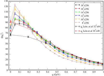
Figure 3: The gluon propagator for all lattices $L_{s}^{3}\times 256$, considering only pure temporal momenta. For comparisation, we also show the $16^{3}\times 48$ and $32^{3}\times 64$ propagators computed in lein99 .

In order to compute the infrared exponent $\kappa$ from the lattice data, we considered fits of the smallest temporal momenta of the gluon dressing function $Z_{gluon}(q^{2})$ to a pure power law with and without polinomial corrections. The results are in table 1. In general, the $\kappa$ values increase with the volume of the lattice. So, our $\kappa$ can be read as lower bounds in the infinite volume figure $\kappa_{\hskip 2.84526pt\infty}$.

$L_{s}$	$z(q^{2})^{2\kappa}$		$z(q^{2})^{2\kappa}(1+aq^{2})$		$z(q^{2})^{2\kappa}(1+aq^{2}+bq^{4})$
$8$	$0.4496^{+22}_{-29}$	2.14	$0.4773^{+37}_{-52}$	0.02	$0.4827^{+75}_{-74}$	0.00
$10$	$0.4650^{+31}_{-37}$	0.10	$0.4827^{+49}_{-68}$	0.25	$0.4765^{+104}_{-99}$	0.14
$12$	$0.4663^{+30}_{-36}$	1.19	$0.4822^{+51}_{-69}$	0.21	$0.4849^{+94}_{-97}$	0.18
$14$	$0.4918^{+26}_{-40}$	0.09	$0.5053^{+52}_{-67}$	0.16	$0.4992^{+100}_{-80}$	0.06
$16$	$0.4859^{+22}_{-24}$	0.40	$0.5070^{+36}_{-50}$	0.44	$0.5131^{+67}_{-64}$	1.03
$18$	$0.5017^{+49}_{-40}$	0.20	$0.5169^{+89}_{-70}$	0.00	$0.514^{+12}_{-15}$	0.00

Table 1: $\kappa$ and $\chi^{2}/d.o.f.$ from fitting the gluon dressing function computed from the different lattices $L_{s}^{3}\times 256$. In all fits, the range of momenta was chosen such that the fits have one degree of freedom. The lowest momentum considered being always the first nonvanishing momentum. The errors shown are statistical and were computed using the bootstrap method, with the number of bootstrap samples being about ten times the number of configurations.

Considering a linear or quadratic dependence on the inverse of the volume for the infrared exponent, we can try to extrapolate the figures of table 1. In what concerns the results for the pure power law fits, they are not described by these functional forms. Using the corrections to the pure power law, one gets values for $\kappa_{\infty}$ in the interval $[0.51,0.56]$; the weighted mean value being $\bar{\kappa}_{\infty}=0.5246(46)$.

On the other hand, one can also extrapolate directly the gluon propagator, as a function of the inverse of the volume, to the infinite volume limit, fitting each timelike momentum propagator separately. Doing so, we are taking the limit $L_{s}\to\infty$ , assuming a sufficient number of points in the temporal direction. Several types of polinomial extrapolations were tried, using different sets of lattices, and we conclude that the data is better described by quadratic extrapolations of the data from the 4th and 5th largest lattices. In figure 4 the two extrapolations of the gluon propagator are shown. For comparisation, we also include the $16^{3}\times 48$ and $32^{3}\times 64$ propagators computed in lein99 .

The values of $\kappa$ extracted from these extrapolated propagators are $\kappa=0.5215(29)$, with a $\chi^{2}/d.o.f.=0.02$, using the largest 5 lattices in the extrapolation, and $\kappa=0.4979(66)$, $\chi^{2}/d.o.f.=0.27$ using the largest 4 lattices. Fitting the extrapolated data to the polinomial corrections to the pure power law, one can get higher values for $\kappa$. Note that the first value is on the top of the value obtained from extrapolating directly $\kappa$ as a function of the volume. In conclusion, one can claim a $\kappa\in[0.49,0.53]$, with the lattice data favouring the right hand side of the interval.

\psfrag{EIXOX}{{\Large$q(GeV)$}}\psfrag{EIXOY}{{\Large$D(q^{2})$}}\includegraphics[width=227.62204pt]{prop_ext.v2.2.ZIR.eps}

Figure 4: The bare extrapolated gluon propagator for momenta below $500MeV$. The errors on the propagator were computed assuming a gaussian error propagation.

III Are DSE fitting forms reproduced by lattice data?

In this section we will try to check if the pure temporal lattice data of the gluon propagator can be described by some functional forms that fitted the solution for the gluon propagator in Landau gauge of the Dyson-Schwinger equations reported in fischer04 ; fischer03 . Only the largest lattices will be considered.

III.1 The infrared region

In the IR region, the continuum DSE solution is well described by the following expressions fischer04 ,

$$Z_{cut}(q^{2})=\omega\left(\frac{q^{2}}{\Lambda_{QCD}^{2}+q^{2}}\right)^{2\kappa}\,,$$ (4)

$$Z_{pole}(q^{2})=\omega\frac{\left(q^{2}\right)^{2\kappa}}{\left(\Lambda_{QCD}^{2}\right)^{2\kappa}+\left(q^{2}\right)^{2\kappa}}\,.$$ (5)

The first functional form has a branch cut in the IR region. The last one has a pole in the IR region.

In what concerns the lattice propagator, both formulas provide good fits up to the maximum of the dressing function — see table 2 and figure 5. However, the measured infrared exponents are larger than those obtained assuming a pure power law for the IR region nossoprd , and support an infrared vanishing gluon propagator.

	Lattice	$q_{max}$	$\kappa$	$\Lambda_{QCD}$	$\chi^{2}/d.o.f.$
$Z_{cut}$	$16^{3}\times 128$	$570$	$0.5117^{+48}_{-46}$	$417^{+8}_{-8}$	$1.25$
	$16^{3}\times 256$	$664$	$0.5090^{+19}_{-20}$	$409^{+4}_{-4}$	$0.71$
	$18^{3}\times 256$	$711$	$0.5320^{+28}_{-30}$	$389^{+5}_{-6}$	$1.14$
$Z_{pole}$	$16^{3}\times 128$	$570$	$0.5100^{+38}_{-31}$	$416^{+6}_{-8}$	$1.15$
	$16^{3}\times 256$	$664$	$0.5077^{+16}_{-17}$	$409^{+4}_{-3}$	$0.69$
	$18^{3}\times 256$	$711$	$0.5266^{+29}_{-21}$	$391^{+3}_{-7}$	$1.09$

Table 2: IR fits. $q_{max}$ is the highest momenta considered in the fit. $q_{max}$ and $\Lambda_{QCD}$ are given in MeV.

\psfrag{EIXOX}{$q(GeV)$}\psfrag{EIXOY}{$q^{2}D(q^{2})$}\includegraphics[width=227.62204pt]{compat18_ir.eps}

Figure 5: The lattice gluon dressing function compared with IR fits.

III.2 The full range of momenta

The lattice propagator, for the full range of pure temporal momenta, was fitted to

$$Z_{fit}(q^{2})~{}=~{}B(q^{2})\,\left(\alpha(q^{2})\right)^{-\gamma}\,,\hskip 5.69046pt\gamma=-13/22\,,$$ (6)

with $B(q^{2})=Z_{pole,cut}$. Two different definitions for the running coupling were considered fischer04 ; fischer03 :

$$\alpha_{P}(q^{2}) = \frac{1}{1+\frac{q^{2}}{\Lambda_{QCD}^{2}}}\bigg{[}\alpha(0)+(q^{2}/\Lambda_{QCD}^{2})\times$$ (7)

$$\frac{4\pi}{\beta_{0}}\Big{(}\frac{1}{\ln(q^{2}/\Lambda_{QCD}^{2})}-\frac{1}{q^{2}/\Lambda_{QCD}^{2}-1}\Big{)}\bigg{]}\,;$$

$$\alpha_{LN}(q^{2}) = \frac{\alpha(0)}{\ln\left[e+a_{1}(q^{2}/\Lambda_{QCD}^{2})^{a_{2}}\right]}\,.$$ (8)

The fits using $\alpha_{\hskip 2.84526ptP}(q^{2})$ (using $\beta_{0}=11$) for the running coupling have a $\chi^{2}/d.o.f.\geq 2$ for $L_{s}=16$. However, for the largest lattice, $18^{3}\times 256$, the data is well described; see table 3 and figure 6.

$18^{3}\times 256$	$\alpha(0)$	$\kappa$	$\Lambda_{QCD}$	$\chi^{2}/d.o.f.$
$B=Z_{cut}$	$10.92^{+13}_{-18}$	$0.5280^{+30}_{-22}$	$549^{+2}_{-3}$	$1.61$
$B=Z_{pole}$	$10.01^{+14}_{-17}$	$0.5263^{+19}_{-22}$	$550^{+2}_{-3}$	$1.54$

Table 3: Fits to all lattice data using $\alpha_{P}(q^{2})$.

Note that only when one uses $B=Z_{pole}$ the $\kappa$ values agree with those from the IR fits. However, $\Lambda_{QCD}$ is not compatible with the IR values. The fitting form differs from the lattice data mainly at the maximum of the dressing function ($\sim 0.8$ GeV).

\psfrag{EIXOX}{{\small$q(GeV)$}}\psfrag{EIXOY}{{\small$q^{2}D(q^{2})$}}\includegraphics[width=227.62204pt]{18_glob_alpha1.eps}

Figure 6: Compatibility between our lattice data and global fits using $\alpha_{P}(q^{2})$.

The lattice data adjusts better to $\alpha_{LN}(q^{2})$ than to the previously considered running coupling. Indeed, looking at the fitting results for our largest lattice (see tables 4 and 5), the values of $\kappa$ and $\Lambda_{QCD}$ are essentially the values obtained in the IR study. Moreover, on overall there is good agreement between the fitting function and the lattice data, see figure 7.

\psfrag{EIXOX}{{\small$q(GeV)$}}\psfrag{EIXOY}{{\small$q^{2}D(q^{2})$}}\includegraphics[width=227.62204pt]{compat_18_alpha2.eps}

Figure 7: Compatibility between our lattice data and global fits using $\alpha_{LN}(q^{2})$.

$B=Z_{cut}$	$\kappa$	$\Lambda_{QCD}$	$a_{1}$	$a_{2}$	$\chi^{2}/d.o.f.$
$16^{3}\times 128$	$0.5435^{+36}_{-41}$	$364^{+4}_{-4}$	$0.0062^{+3}_{-3}$	$2.44^{+2}_{-1}$	$1.82$
$16^{3}\times 256$	$0.5244^{+21}_{-15}$	$374^{+2}_{-2}$	$0.0072^{+3}_{-3}$	$2.42^{+1}_{-1}$	$1.73$
$18^{3}\times 256$	$0.5368^{+25}_{-24}$	$381^{+3}_{-4}$	$0.0067^{+4}_{-5}$	$2.55^{+2}_{-2}$	$1.23$

Table 4: Fits to all lattice data using $\alpha_{LN}(q^{2})$ and $B=Z_{cut}$.

$B=Z_{pole}$	$\kappa$	$\Lambda_{QCD}$	$a_{1}$	$a_{2}$	$\chi^{2}/d.o.f.$
$16^{3}\times 128$	$0.5335^{+23}_{-26}$	$373^{+3}_{-3}$	$0.0081^{+3}_{-3}$	$2.36^{+2}_{-2}$	$1.65$
$16^{3}\times 256$	$0.5217^{+14}_{-14}$	$377^{+2}_{-2}$	$0.0082^{+3}_{-3}$	$2.36^{+1}_{-1}$	$1.61$
$18^{3}\times 256$	$0.5300^{+17}_{-21}$	$388^{+3}_{-3}$	$0.0085^{+6}_{-4}$	$2.46^{+2}_{-3}$	$1.20$

Table 5: Fits to all lattice data using $\alpha_{LN}(q^{2})$ and $B=Z_{pole}$.

The running coupling at zero momentum can be measured from $\alpha_{LN}(q^{2})$ sardenha ; dublin and is related with the high momentum behaviour of the running coupling, $\alpha(0)~{}=~{}(4\pi/\beta_{0})\,a_{2}\,$. The measured $\alpha(0)$ are reported in table 6. Note that the values from the $16^{3}\times 128$ and $16^{3}\times 256$ data agree within one standard deviation. Furthermore, $\alpha(0)$ increases with $L_{s}$ and the fitted values reported in table 6 are around the original DSE estimation for $\alpha(0)=2.972$ lerche .

$\alpha(0)$	$Z_{cut}$	$Z_{pole}$
$16^{3}\times 128$	$2.79^{+2}_{-1}$	$2.70^{+2}_{-2}$
$16^{3}\times 256$	$2.77^{+1}_{-1}$	$2.70^{+1}_{-1}$
$18^{3}\times 256$	$2.91^{+2}_{-3}$	$2.81^{+2}_{-3}$

Table 6: Values of $\alpha(0)$ measured from $\alpha_{LN}(q^{2})$.

IV Gribov copies effects in the propagators

The propagators are gauge dependent quantities. To compute them, one has to choose a gauge. For the Landau gauge on the lattice, the procedure consists in maximizing the functional,

$$F_{U}[g]~{}=~{}C_{F}\sum_{x,\mu}\,\mbox{Re}\,\{\,\mbox{Tr}\,[g(x)U_{\mu}(x)g^{\dagger}(x+\hat{\mu})]\,\}$$ (9)

It is well known that this functional has, in general, several maxima, the Gribov copies gribov . To properly define a non-perturbative gauge fixing, one should choose the gauge transformation $g(x)$ that globally maximizes (9). This is a global optimization problem and it is not easy to find the global maximum of (9). In most studies of the gluon and ghost propagators one chooses a local maximum of (9), hoping that the Gribov copy effects in the propagators are small.

On the lattice, several studies reported Gribov effects in the ghost propagator (see, for example, cucc97 ; stern05 ; madrid , and the next section), but it is generally accepted that Gribov copies do not change significantly the gluon propagator.

However, there are some studies reporting Gribov copy effects in the gluon propagator. In npb04 , the problem of the Gribov copies effects on the gluon propagator was studied, and some differences were found. It was claimed a two to three $\sigma$ effect due to Gribov copies in the low momentum region. Furthermore, it was observed, by sorting the different Gribov copies according to the value of the gauge fixing functional, that the propagator for the lowest momenta behaves monotonically as a function of $<F_{U}>$: for zero momentum, the propagator increases with $<F_{U}>$, and for some small non-zero momenta the propagator decreases with $<F_{U}>$. There is also a study bbmpm05 where the authors claim that the enlargement of the gauge orbits allows for Gribov effects in the gluon propagator.

In what concerns asymmetric lattices, CEASD gauge fixing method ceasd was applied to the $16^{3}\times 128$ configurations. This global optimization method for Landau gauge fixing combines a genetic algorithm with a local gauge fixing method, aiming to find the global maximum of (9). The obtained gluon propagator was compared with the one computed from a local maximum of (9); this local maximum is obtained using the local gauge fixing method described in davies . In fig. 8, we can see the ratio between the two propagators.

\psfrag{EIXOX}{{\small$\hat{n}_{t}$}}\psfrag{EIXOY}{{\small$D_{ID}/D_{CEASD}$}}\includegraphics[width=227.62204pt]{gribov.eps}

Figure 8: Gribov copy effects in the gluon propagator computed from $16^{3}\times 128$ configurations.

Although there are many momenta for which the ratio is not compatible with one, we cannot conclude in favour of any systematic effect.

V Ghost propagator and running coupling constant

V.1 Ghost propagator

For our smallest lattices ($10^{3}\times 256$, $12^{3}\times 256$, $16^{3}\times 128$), we have computed the ghost propagator madrid ,

$$G^{ab}(q)=-\delta^{ab}G(q^{2})$$ (10)

using both a point source method suman (we averaged over 7 different point sources to get a better statistics), and a plane-wave source cucc97 . In both cases we used the preconditioned conjugate algorithm, as described in stern05 . The advantage of using a plane-wave source being that the statistical accuracy is much better, but we can only obtain one momentum component at a time. Using a point source method one can get all the momenta in once, but with larger statistical errors.

In figures 9 and 10 it is shown the ghost dressing function $Z_{ghost}(q^{2})$ for $12^{3}\times 256$ and $16^{3}\times 128$ computed with both methods. For the $12^{3}\times 256$, the point source data is not smooth for a large range of momenta. This is true also for $10^{3}\times 256$ lattice , but this effect is significantly reduced for $16^{3}\times 128$. In what concerns finite volume effects, we see differences, in the infrared, between pure temporal and pure spatial data, as in the gluon case.

\psfrag{EIXOX}{$q(GeV)$}\psfrag{EIXOY}{ $Z_{ghost}(q^{2})$}\includegraphics[width=227.62204pt]{dress.12.3.256.eps}

Figure 9: Bare ghost dressing function for a $12^{3}\times 256$ lattice; “p2p” (“pws”) stands for the ghost components computed using a point (plane wave) source.

\psfrag{EIXOX}{$q(GeV)$}\psfrag{EIXOY}{$Z_{ghost}(q^{2})$}\includegraphics[width=227.62204pt]{dress.16.3.128.eps}

Figure 10: Bare ghost dressing function for a $16^{3}\times 128$ lattice.

In figure 11 one can see the ghost dressing function only for the plane-wave data. As in the gluon case, we are able to evaluate the effect of Gribov copies on the lattice $16^{3}\times 128$ by considering different gauge fixing methods. One can see clear effects of Gribov copies, as expected from other studies cucc97 ; stern05 . Also, we see finite volume effects if one compares propagators computed from lattices with different spatial sizes.

In what concerns the infrared region, we were unable to fit a pure power law, even considering polinomial corrections madrid . This negative result can be due either to the finite volume effects caused by the small spatial extension of our lattices, or to an insufficient number of points in the infrared region — note that for the ghost propagator, the pure power law lacks validity well below 200 MeV (see figure 1).

\psfrag{EIXOX}{$q(GeV)$}\psfrag{EIXOY}{$Z_{ghost}(q^{2})$}\includegraphics[width=227.62204pt]{cucc.eps}

Figure 11: Bare ghost dressing function for all lattices. The data were computed using a plane wave method.

V.2 Running coupling constant

Using the gluon and ghost dressing functions, one can define a running coupling constant as

$$\alpha_{S}(q^{2})=\alpha(\mu^{2})Z_{ghost}^{2}(q^{2})Z_{gluon}(q^{2}).$$ (11)

The DSE infrared analysis predicts a running coupling constant at zero momentum different from zero, $\alpha_{S}(0)=2.972$ lerche . On the other hand, the DSE solution on a torus dsetorus , and results from lattice simulations stern05 ; furui1 ; furui2 ; madrid , shows a decreasing coupling constant for small momenta. Using an asymmetric lattice allow us to study smaller momenta having in mind to provide, at least, a hint to this puzzle.

Again, our lattice data shows finite volume effects, if one compares pure temporal and pure spatial momenta, see figure 12. Comparing the results for all available lattices (plane-wave source), see figure 13, we can see, as in the ghost case, finite volume effects, and clear Gribov copies effects.

\psfrag{EIXOX}{$q(GeV)$}\psfrag{EIXOY}{$\alpha(q^{2})/\alpha(\mu^{2})$}\includegraphics[width=227.62204pt]{alpha.16.3.128.eps}

Figure 12: Running coupling constant for a $16^{3}\times 128$ lattice.

\psfrag{EIXOX}{$q(GeV)$}\psfrag{EIXOY}{$\alpha(q^{2})/\alpha(\mu^{2})$}\includegraphics[width=227.62204pt]{alpha.cucc.eps}

Figure 13: Running coupling constant for all lattices. The data were computed using a plane wave method.

In what concerns the infrared behaviour, we tried to fit the lowest momenta to a pure power law, $(q^{2})^{\kappa_{\alpha}}$. We concluded that this power law is only compatible with the data from $16^{3}\times 128$ lattice, gauge fixed with CEASD method, giving $\kappa_{\alpha}\sim 0.688$, with $\chi^{2}/d.o.f.\sim 0.011$. The reader should be aware that it is also possible, in some cases, to fit the infrared data to $\alpha(0)(1+aq^{2}+\ldots)$ and get a $\alpha(0)\neq 0$. Therefore, we can not give a definitive answer about the behaviour of the running coupling constant for $q=0$. Note, however, that $\alpha_{S}(q^{2})$ for the smallest momenta, seems to increase as a function of the volume.

VI Conclusions

In this work asymmetric lattices were used to study the infrared behaviour of QCD propagators.

In what concerns the gluon propagator, the lattice data is well described by a pure power law $(q^{2})^{2\kappa}$ for momenta below 150 MeV. The value of the infrared exponent increases with the volume, so our $\kappa$’s can be read as lower bounds of the infinite volume figure. Extrapolating the gluon propagator to the infinite volume limit, assuming a sufficient temporal size of our lattices, one gets $\kappa\in[0.49,0.53]$. Unfortunately, we can not give a definitive answer about the behaviour of the gluon propagator at zero momentum. Note, however, that the lattice data favours the right hand side of the given interval, and that using other fitting forms and a larger range of momenta, one always get $\kappa>0.5$.

In what concerns the ghost propagator, we were not able to extract a pure power law on the available results. We observed finite volume effects and clear Gribov copies effects on this propagator, in agreement with other studies.

Finally, we observed a decreasing running coupling for low momenta, in agreement with previous simulations.

References

- (1) R. Alkofer, L. von Smekal, Phys. Rept. 353 (2001) 281 [hep-ph/0007355].
- (2) C. Lerche, L. von Smekal, Phys. Rev. D65 (2002) 125006 [hep-ph/0202194].
- (3) J. M. Pawlowski, D. F. Litim, S. Nedelko, L. von Smekal, Phys. Rev. Lett. 93 (2004) 152002 [hep-th/0312324].
- (4) C. S. Fischer, H. Gies, JHEP 0410 (2004) 048 [hep-ph/0408089].
- (5) D. Zwanziger, Phys. Rev. D67 (2003) 105001 [hep-th/0206053].
- (6) C. S. Fischer, M. R. Pennington, Phys. Rev. D73 (2006) 034029 [hep-ph/0512233].
- (7) O. Oliveira, P. J. Silva, AIP Conf. Proc. 756 (2005) 290 [hep-lat/0410048].
- (8) P. J. Silva, O. Oliveira, PoS(LAT2005)286 [hep-lat/0509034].
- (9) O. Oliveira, P. J. Silva, PoS(LAT2005)287 [hep-lat/0509037].
- (10) P. J. Silva, O. Oliveira, Phys. Rev. D74 (2006) 034513 [hep-lat/0511043].
- (11) O. Oliveira, P. J. Silva, hep-lat/0609027.
- (12) O. Oliveira, P. J. Silva, PoS(LAT2006)075 [hep-lat/0609069].
- (13) A. Cucchieri, T. Mendes, Phys. Rev. D73 (2006) 071502 [hep-lat/0602012].
- (14) Andre Sternbeck, PhD thesis, hep-lat/0609016.
- (15) R. Alkofer, W. Detmold, C.S. Fischer, P. Maris, Phys. Rev. D70 (2004) 014014 [hep-ph/0309077].
- (16) C. S. Fischer, R. Alkofer, Phys. Rev. D67 (2003) 094020 [hep-ph/0301094].
- (17) A. Cucchieri, Nucl. Phys. B508 (1997) 353 [hep-lat/9705005].
- (18) A. Sternbeck, E.-M. Ilgenfritz, M. Muller-Preussker, A. Schiller, Phys. Rev. D72 (2005) 014507 [hep-lat/0506007].
- (19) V. N. Gribov, Nucl. Phys. B139 (1978) 1.
- (20) P. J. Silva, O. Oliveira, Nucl. Phys. B690 (2004) 177 [hep-lat/0403026].
- (21) I. L. Bogolubsky, G. Burgio, V. K. Mitrjushkin, M. Mueller-Preussker, Phys.Rev. D74 (2006) 034503 [hep-lat/0511056].
- (22) O.Oliveira, P.J.Silva, Comp. Phys. Comm. 158 (2004) 73 [hep-lat/0309184].
- (23) H. Suman, K. Schilling, Phys.Lett. B373 (1996) 314 [hep-lat/9512003].
- (24) C. S. Fischer, B. Gruter, R. Alkofer, Annals Phys. 321 (2006) 1918 [hep-ph/0506053].
- (25) D. B. Leinweber, J. I. Skullerud, A. G. Williams, and C. Parrinello, Phys. Rev. D 60, 094507 (1999);61, 079901 (2000) [hep-lat/9811027].
- (26) S. Furui, H. Nakajima, Phys. Rev. D 69, 074505 (2004) [hep-lat/0305010].
- (27) S. Furui, H. Nakajima, Phys. Rev. D 70, 094504 (2004) [hep-lat/0403021].
- (28) C. H. T. Davies, G. G. Batrouni, G. P. Katz, A. S. Kronfeld, G. P. Lepage, P. Rossi, B. Svetitsky and K. G. Wilson, Phys. Rev.D37 (1988) 1581.