On the Locality and Scaling of Overlap Fermions at Coarse Lattice Spacings

Abstract

The overlap fermion offers the considerable advantage of exact chiral symmetry on the lattice, but is numerically intensive. This can be made affordable while still providing large lattice volumes, by using coarse lattice spacing, given that good scaling and localization properties are established. Here, using overlap fermions on quenched Iwasaki gauge configurations, we demonstrate directly that, with appropriate choice of negative Wilson’s mass, the overlap Dirac operator’s range is comfortably small in lattice units for each of the lattice spacings 0.20 fm, 0.17 fm, and 0.13 fm (and scales to zero in physical units in the continuum limit). In particular, our direct results contradict recent speculation that an inverse lattice spacing of $1\,{\rm GeV}$ is too low to have satisfactory localization. Furthermore, hadronic masses (available on the two coarser lattices) scale very well.

UK/06-11

1 Locality

In the last several years the use of the overlap lattice fermion has become more popular because the conceptual and technical clarity that results from its exact chiral symmetry is seen to overcome its superficially higher computational cost as compared to conventional lattice formulations of the fermion. Furthermore, the disparity in numerical intensity can be mitigated by using coarse lattice spacing, given that good scaling and localization properties are established.

Hernández, Jansen, and Lüscher [1] have shown numerically that Neuberger’s overlap operator is local on pure-glue backgrounds (using the Wilson gauge action on fine lattices). The decay rate (inverse of the range) $r_{\rm ov}^{-1}$ of the overlap kernel can be interpreted as the mass of unphysical degrees of freedom. Recently, Golterman, Shamir, and Svetitsky [2] have argued that, in practice, these can be dangerously light. They provide an indirect estimate for pure-gauge ensembles (for Wilson, Iwasaki, and DBW2 gauge actions) at different lattice spacings. For cutoff $a^{-1}\sim 2\,{\rm GeV}$ they estimate $r_{\rm ov}^{-1}\approx 0.4\times 2{\rm GeV}=800\,{\rm MeV}$, which is acceptably large. For $a^{-1}\sim 1\,{\rm GeV}$, however, they raise an alarm with their estimate of $r_{\rm ov}^{-1}\approx 0.25\times 1{\rm GeV}=250\,{\rm MeV}$ for the Wilson case, $270\,{\rm MeV}$ for Iwasaki, and $320\,{\rm MeV}$ for DBW2.

However, their estimate is indirect, and follows a chain of approximations at the end of which they assume that $r_{\rm ov}^{-1}\approx\lambda_{c}^{-1}$, where $\lambda_{c}$ is the “mobility edge” of a Dirac spectrum. Here we come to a very different conclusion using the most direct approach which takes advantage of the fact that it is not expensive to calculate, rather than estimate, $<D_{\rm ov}(x,y)>$. (By comparison, it would be much more expensive to calculate the overlap propagator $D_{\rm ov}^{-1}$ which must be computed by nested iterations.)

In contrast to the results of Golterman, Shamir, and Svetitsky [2], who speculate that overlap simulations with a cutoff of $1\,{\rm GeV}$ (such as [3]) might have a range as long as 4 lattice units, here we show directly that such is not the case; with appropriate choice of negative Wilson’s mass, the range is about 1 lattice unit (in Euclidean distance or 2 units of “taxi-driver” distance). All is well.

A preliminary version of these results was presented in [4]. Durr, Hoelbling, and Wenger [5] came to similar conclusions using the overlap operator with a UV filtered (“thick link”) Wilson kernel.

1.1 Lattice Details

We use the renormalization-group-improved Iwasaki [6] gauge action, on three different lattices; for each, the lattice size, lattice spacing, and number of configurations used are tabulated in Table 1.

$N_{s}\times N_{t}$	$a(r_{0})$	$a(f_{\pi})$	$N_{\rm cfg}$
$16^{3}\times 28$	$0.175\,{\rm fm}$	$0.20\,{\rm fm}$	$300/10$
$20^{3}\times 32$	$0.153\,{\rm fm}$	$0.17\,{\rm fm}$	$98/10$
$28^{3}\times 44$	$0.113\,{\rm fm}$	$0.13\,{\rm fm}$	$0/10$

Table 1: Lattice size, lattice spacing (as set by the Sommer parameter $r_{0}$ [7]), lattice spacing (as set by $f_{\pi}(m_{\pi})$ [3]), and number of configurations (for scaling/locality).

For the associated scaling study of hadron masses, we use the overlap fermion [8, 9] and massive overlap operator [10, 11, 12, 13]

$$D(m_{0})=(\rho+\frac{m_{0}a}{2})+(\rho-\frac{m_{0}a}{2})\gamma_{5}\epsilon(H)$$ (1)

where $\epsilon(H)=H/\sqrt{H^{2}}$, $H=\gamma_{5}D_{w}$, and $D_{w}$ is the usual Wilson fermion operator, except with a negative mass parameter $-\rho=1/2\kappa-4$ in which $\kappa_{c}<\kappa<0.25$; we take $\kappa=0.19$ in our calculation which corresponds to $\rho=1.368$. For the locality study, we set $m_{0}=0$ to look at the properties of the massless operator $D(0)$. Complete details are described in [3].

1.2 Locality as Measured by Taxi-Driver Distance

It has been convenient to discuss locality in terms of a “taxi-driver” distance [1], rather than the standard Euclidean distance.

$$r_{\rm TD}\equiv||x-y||_{1}=\sum_{\mu}|x_{\mu}-y_{\mu}|$$ (2)

The locality of the overlap operator is then studied by plotting the quantity $\mathcal{D}_{\rm max}(r)$ ($f(r)$ in the notation of [1]) as a function of the taxi-driver distance for a localized source, $\psi_{\alpha}(x)=\delta(x)\delta_{\alpha\beta}$ for fixed Dirac-color index $\beta$.

$$\mathcal{D}_{\rm max}(r)\equiv\max\{||D\psi(x)||\,\,|\,\,\sum_{\mu}x_{\mu}=r\}$$ (3)

For large $r$, the Dirac-overlap operator decays exponentially with decay rate $\nu=r_{\rm ov}^{-1}$, where $r_{\rm ov}$ is the range (characteristic decay distance) measured in lattice units.

1.3 Results

In Fig. 1, we plot $\mathcal{D}_{\rm max}(r)$ as a function of taxi-driver distance for the $16^{3}\times 28$ lattice. At large distances, we fit to an exponentially decreasing function to extract the range $r_{\rm ov}$.

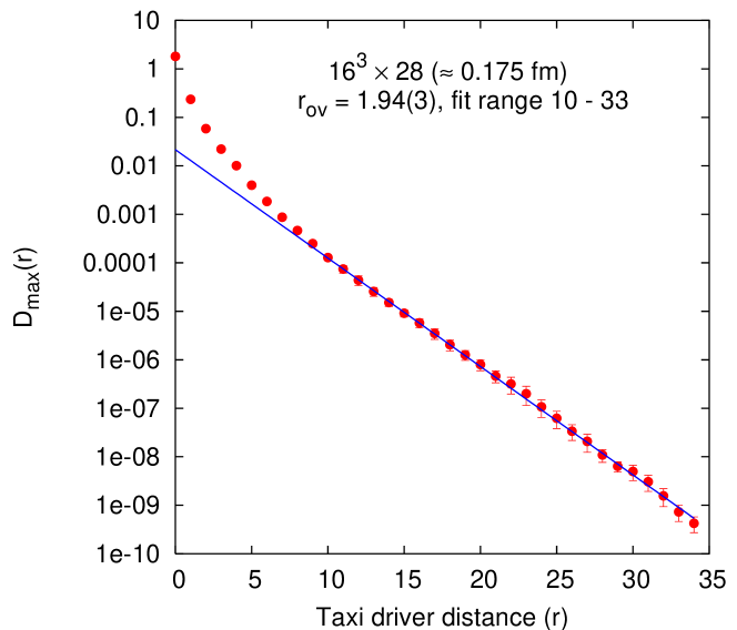
Figure 1: For the $16^{3}\times 28$ lattice, the expectation value of $\mathcal{D}_{\rm max}(r)$ as a function of the taxi-driver distance, $r$. For large $r$, $\mathcal{D}_{\rm max}(r)$ falls exponentially, with range $r_{\rm ov}$. The fitted value of $r_{\rm ov}$ is shown with the chosen fit interval.

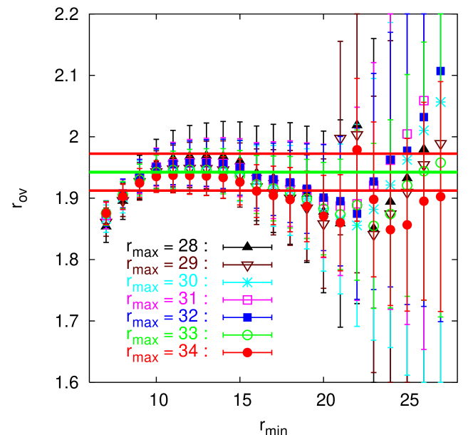
Figure 2: For the $16^{3}\times 28$ lattice, the fitted values of $r_{\rm ov}$ for various choices of fit interval ($r_{\rm min}$,$r_{\rm max}$) are displayed as a function of $r_{\rm min}$ for each $r_{\rm max}$, to help choose the best fit.

To help choose the optimal fit interval, we display in Fig. 2 the fitted values of $r_{\rm ov}$ for various choices of fit interval ($r_{\rm min}$,$r_{\rm max}$) as a function of $r_{\rm min}$ for each $r_{\rm max}$. In analogy with one’s experience fitting the ground state mass of a two-point hadronic correlation function, for sufficiently large $r_{\rm max}$ one would expect to see the fitted value of the range $r_{\rm ov}$ increase (since $1/r_{\rm ov}$ is a mass) toward a plateau as $r_{\rm min}$ is increased. And as $r_{\rm min}$ is increased further one would expect to see the plateau disappear into noise. This is what we see in Fig. 2. We choose the least value of $r_{\rm min}$ for which the plateau is established, and a value $r_{\rm max}$ for which the fit errors fairly represent the dispersion of results from various other acceptable fit intervals.

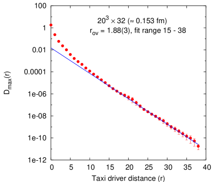
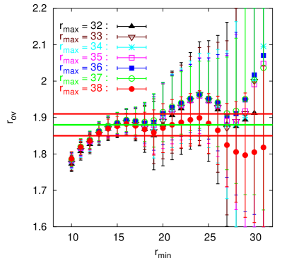
Figure 3: Same as figures 1 and 2 but for the $20^{3}\times 32$ lattice.

In Fig. 3 (left pane), we plot $\mathcal{D}_{\rm max}(r)$ as a function of taxi-driver distance for the $20^{3}\times 32$ lattice, showing the fit of $r_{\rm ov}$ for this lattice. The fit interval is chosen upon analysis of Fig. 3 (right pane).

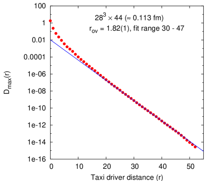
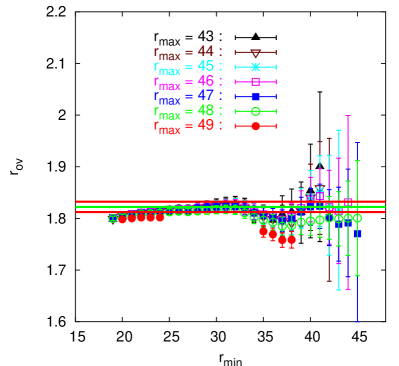
Figure 4: Same as figures 1 and 2 but for the $28^{3}\times 44$ lattice.

Finally, in Fig. 4 (left pane), we plot $\mathcal{D}_{\rm max}(r)$ as a function of taxi-driver distance for the $28^{3}\times 44$ lattice, showing the fit of $r_{\rm ov}$ for this lattice. Again, the fit interval is chosen from analysis of an “$r_{\rm min}$” plot, Fig. 4 (right pane).

Our fitted values of $r_{\rm ov}$ for each of our three lattices are tabulated in Table 2. We note that our results are similar to the results of Hernández, Jansen and Lüscher [1] obtained on finer lattices for the overlap operator ($\rho=1.4$) with Wilson action at $\beta=6.0$, $6.2$, and $6.4$; they find $r_{\rm ov}=\nu^{-1}=1/0.49\approx 2.0$.

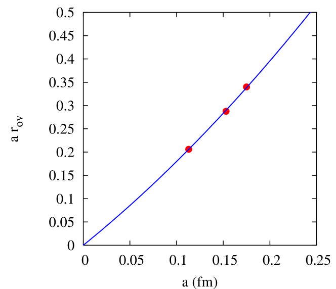
Figure 5: Taxi driver range in physical units (fm) as a function of lattice spacing ($r_{0}$ scale). The range is small even at coarse lattice spacing and trends to zero in the continuum limit.

$a(r_{0})$	$r_{\rm ov}$
$0.175\,{\rm fm}$	$1.94(3)$
$0.153\,{\rm fm}$	$1.88(3)$
$0.113\,{\rm fm}$	$1.82(1)$

Table 2: The range (taxi driver metric) for three lattice spacings. It is less than two lattice units on a lattice as coarse as $0.20\,{\rm fm}$ ($f_{\pi}$ scale).

Furthermore, it is gratifying to see that even for our coarsest lattice, $0.20\,{\rm fm}$ ($f_{\pi}$ scale), the measured range is less than two lattice units. In Fig. 5 we plot the range in physical units as a function of lattice spacing ($r_{0}$ scale). It trends to zero in the continuum limit; a quadratic fit restrained to go through the origin has a satisfactory $\chi^{2}/dof=0.31$.

1.3.1 Wrap-around Effects

In this section, we delve further into some of the details used in extracting the overlap range. In particular, the raw data needs to be cut in order to reduce wrap-around effects to an acceptable and conservative level.

Our raw data is displayed in Fig. 6. This includes data at all taxi-driver distances except for some at very large distances on the largest lattice where the numerical precision used in calculating $D$ may be inadequate.

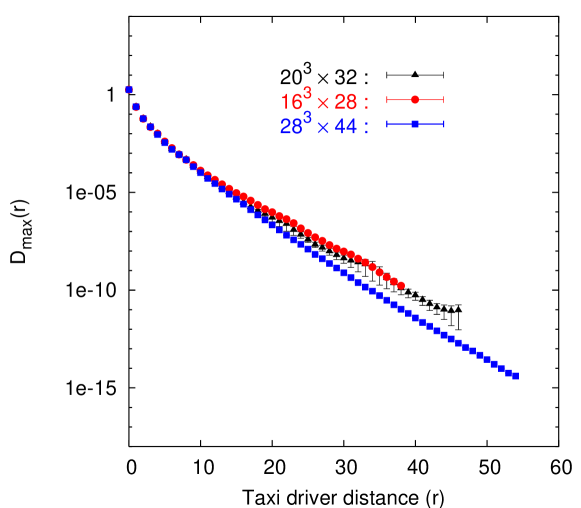
Figure 6: Raw data (at all taxi-driver distances except for some at very large distances on the largest lattice where the precision is inadequate). This includes distances contaminated by wrap-around effects.

This raw data includes values at large distances which are contaminated by wrap-around effects, due to the finite volume of the lattices; these must be accounted for in order to extract the range of the overlap operator. To quantify the extent of the wrap-around effects, we consider first a subset of data restricted to be along the $t$ axis. If the lattice were infinite in time extent, one could extract the inverse range $\nu\equiv r_{\rm ov}^{-1}$ by defining an “effective inverse range” $\nu_{\rm exp}(t)\equiv\ln\left(D\psi(t-1)/D\psi(t)\right)$ (like an “effective mass” [14]), based on the fit-model $D\psi(t)\sim\exp{(-\nu t)}$ for the exponential tail. At large time $t$, a “plateau” is seen where $\nu_{\rm exp}(t)$ is independent of $t$. However, for a finite lattice of time extent $T$, the exponential fit model breaks down due to additive contributions $\sim\exp{\left(-\nu(T-t)\right)}$ from wrap around and, instead, the fit model $D\psi(t)\sim\cosh{(-\nu(t-T/2))}$ is appropriate for times $t$ near the middle of the lattice ($1\ll t\ll T$). But still, one can define another “effective inverse range” $\nu_{\rm cosh}(t)$, appropriate for the new fit model; this forms a plateau in the middle of the periodic lattice. For small $t$ on a periodic finite lattice, $\nu_{\rm exp}(t)\approx\nu_{\rm cosh}(t)$ with exponentially small difference as the wrap-around effects are negligible. But near the middle of the lattice, while the cosh effective range forms a plateau, the exponential effective range deviates exponentially due to the wrap-around effects.

One can then define a figure of merit $\left(\nu_{\rm cosh}(t)-\nu_{\rm exp}(t)\right)/\nu_{\rm cosh}(t)$. For the $28^{3}\times 44$ lattice, this is plotted (and labeled “(cosh-exp)/cosh”) in Fig. 7 with either a linear (left pane) or logarithmic scale (right pane). This figure of merit can be used to identify those times $t$ which are too close to the middle of the lattice and which suffer substantial contributions from wrap-around effects.

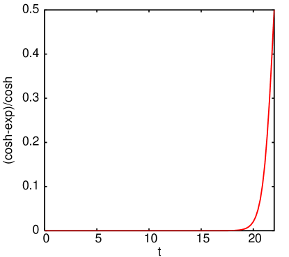
Figure 7: Data restricted to be along the $t$ axis reveals the extent of the wrap-around artifacts (for the $28^{3}\times 44$ lattice). A figure of merit $\left(\nu_{\rm cosh}(t)-\nu_{\rm exp}(t)\right)/\nu_{\rm cosh}(t)$ is plotted on a linear scale (left pane) and on a logarithmic scale (right pane). A threshold of 1% contamination occurs at two sites from the lattice midpoint.

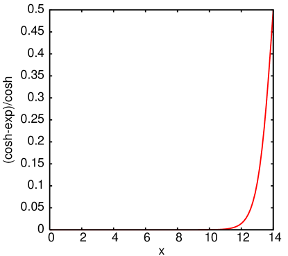
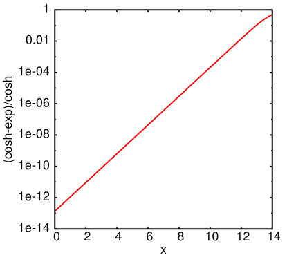
Figure 8: Same as for Fig. 7 but for data restricted to be along the $x$ axis.

Since our lattices are asymmetric, we repeat the procedure for data restricted to lie along the $x$ axis; the corresponding figure of merit is plotted in Fig. 8. These graphs reveal the extent of the wrap-around artifacts. To reduce them to a harmless level, we choose to cut the data using a threshold of 1% contamination. From figures Fig. 7 and Fig. 8, we see that this occurs at two sites from the lattice midpoint (for either the $t$ or $x$ direction).

We define $cut=0$ to mean that no data is removed, and likewise define $cut=1$ to mean that data at a point with time coordinate $t$ at the midpoint of the lattice $t=T/2$ are removed, but data at $|t-T/2|=1,2,\cdots$ are retained. From Fig. 7 and Fig. 8 then, we find that $cut=3$ (for the $28^{3}\times 44$ lattice).

Returning the the full data set with lattice points specified by coordinates $(x,y,z,t)$, we demand that data with any Cartesian component within a distance of $cut-1=2$ of the midpoint be rejected to ensure that the data that survives the cut is uncontaminated at about the 1% level. Similarly, for the $20^{3}\times 32$ lattice, we find that $cut=2$ corresponds to the 1% threshold. For the $16^{3}\times 28$ lattice, $cut=1$.

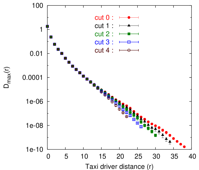
Figure 9: For the $16^{3}\times 28$ lattice, the expectation value of $\mathcal{D}_{\rm max}(r)$ as a function of taxi-driver distance, $r$, for all data ($cut=0$), and for data discarded if within $cut-1$ of any lattice midpoint. $cut=1$ is chosen as our central value wherein wrap-around effects are smaller than 1%. This is the worst-case scenario; cutting any more would reduce the fitted decay distance $r_{\rm ov}$ further.

Next, we investigate the consequences of choosing various values for the cut. As $cut$ increases, more data is discarded and wrap-around effects are further diminished, but less data is available at large distances from which to extract the range. In Fig. 9 we plot, for the $16^{3}\times 28$ lattice, the expectation value of $\mathcal{D}_{\rm max}(r)$ as a function of taxi-driver distance, $r$, for all data ($cut=0$), and for data discarded if within $cut-1$ of any lattice midpoint. We have chosen $cut=1$ as our preferred value wherein wrap-around effects are smaller than 1%. This is a conservative choice — the worst-case scenario; cutting any more would reduce the fitted decay distance $r_{\rm ov}$ further, and runs the risk of increasing the systematic error of the fitted range due to discarding data in the large-distance plateau.

1.4 Locality as Measured by Euclidean Distance

We conclude that it is perfectly acceptable to simulate overlap fermions with lattice spacing as coarse as $0.20\,{\rm fm}$ ($f_{\pi}$ scale), since for this we find that the range is not greater than two lattice units when measured in taxi-driver distance. In fact, the situation is even better than it seems. To see this, we consider the more familiar standard Euclidean metric

$$r_{\rm E}\equiv||x-y||_{2}=\sqrt{\sum_{\mu}|x_{\mu}-y_{\mu}|^{2}}$$ (4)

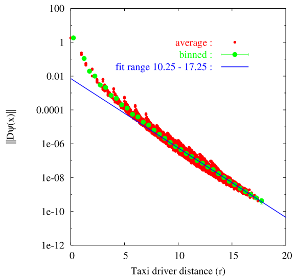
Figure 10: For the $16^{3}\times 28$ lattice, the expectation value of $||D\psi(x)||$ versus Euclidean distance $r$ (for data cut to remove wrap-around effects). Data plotted in red (darker shade of gray) are averages over configurations; however, the maximum has not been taken over points with equal Euclidean distance. The (many fewer) green (lighter shade of gray) points are averages of these within bins of width $0.5$. For large $r$, these averages fall exponentially, with range $r_{\rm ov}$.

In Fig. 10 we plot, for our coarsest lattice, $||D\psi(x)||$ (for localized source $\psi_{\alpha}(x)=\delta(x)\delta_{\alpha\beta}$ with fixed Dirac-color index $\beta$) versus the Euclidean distance. Here all data (averaged over configurations) are shown as the profuse red points, without a maximum taken over points with equal Euclidean distance, in contrast to Eq. 3. Said maxima do not form as smooth an envelope as in the taxi-driver case; there are many more possible values of Euclidean distance than taxi-driver distance, which leads to more jitter and sensitivity to violations of rotational symmetry. Nevertheless, data are still clearly contained with a worst-case decay rate.

To obtain an estimate of the range in this case, the data are first smoothed by averaging over bins of width $0.5$ (in lattice Euclidean distance) to obtain $\mathcal{D}_{\rm avg}(r)$. (Taking the maximum over bins, in the spirit of Eq. 3 results in an envelope which is too sensitive to the choice of bin size and position.) The resulting data do have a smooth dependence as a function of Euclidean distance, and exhibit an exponential tail which is then fitted.

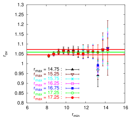
Figure 11: For the $16^{3}\times 28$ lattice, the fitted values of $r_{\rm ov}$ for various choices of fit interval ($r_{\rm min}$,$r_{\rm max}$) are displayed as a function of $r_{\rm min}$ for each $r_{\rm max}$, to help choose the best fit.

As was done for the taxi-driver case, the fit range is chosen from various alternatives, as shown in Fig. 11. As before, we choose the least value of $r_{\rm min}$ for which the plateau is clearly and definitely established, and a value $r_{\rm max}$ for which the fit errors fairly represent the dispersion of results from various other acceptable fit intervals.

Choosing a fit range with the above criteria, we fit the tail of the function with a decaying exponential to extract the range for each of our three lattices. We tabulate the results in Table 3. In comparing Tables 2 and 3, note that although the two ranges (taxi-driver and Euclidean) differ by a factor of about two, they are quite compatible heuristically; on a $L^{4}$ hypercube, the maximum taxi-driver distance is $4(L/2)=2L$, and the maximum Euclidean distance is $\sqrt{4(L/2)^{2}}=L$.

$a$	$r_{\rm ov}$
$0.175\,{\rm fm}$	$1.06(1)$
$0.153\,{\rm fm}$	$0.98(2)$
$0.113\,{\rm fm}$	$0.94(6)$

Table 3: The range (Euclidean metric) at three values of lattice spacing. It is less than about 1 lattice unit with lattice spacing as coarse as $0.20\,{\rm fm}$ ($f_{\pi}$ scale).

So even at lattices as coarse as $a=0.20\,{\rm fm}$ ($f_{\pi}$ scale), the range is about 1 lattice unit (measured using Euclidean distance, or 2 units using taxi-driver distance). No unphysical degrees of freedom are induced at distances longer than the lattice cutoff.

1.5 A Check: Free Field

We include here a useful check of our calculations and expectations. With the same program used for the interacting-field case, we have calculated $D(x,y)$ for source $y$ and sink $x$ for the free-field case, that is, with all $SU(3)$ matrices on the links set equal to the identity matrix. We compared the output with an alternative calculation in terms of Fourier series and found complete agreement. As an aside, we then repeated the calculation of the overlap operator range for the free-field case.

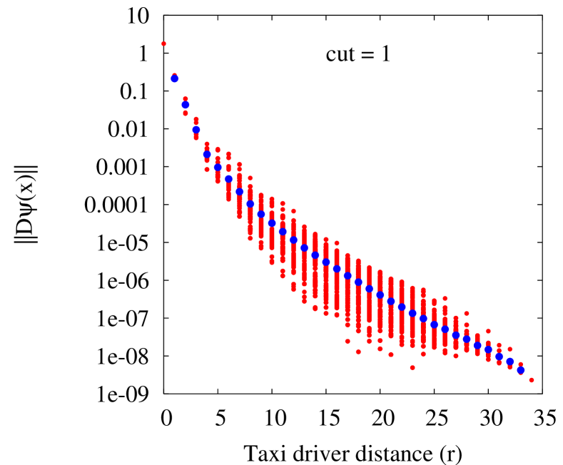
Figure 12: Free field case for the $16^{3}\times 28$ lattice (cut=1). $||D\psi(x)||$ is displayed (red points) for all coordinates; the average $\mathcal{D}_{\rm avg}(r)$ over all equivalent points with a given taxi-driver distance $r$ is shown in blue.

For the $16^{3}\times 28$ lattice, we display in Fig. 12 a plot for the free-field case similar to that of the interacting case (Fig. 1), and using the same value to cut the data. An important difference, however, is that we display the value of $||D\psi(x)||$ for all points, that is, the maximum is not taken as in Eq. 3. One sees in Fig. 12 that, in contrast to the interacting case, the maximum values for each taxi-driver distance do not form a smooth envelope. Presumably, this is a consequence of the lack of rotational invariance for the free case. This lack of smoothness makes it difficult to obtain a quantitative estimate of the range. A much smoother curve is obtained by taking the average (mean) $\mathcal{D}_{\rm avg}(r)$, rather than the maximum, of all equivalent points which have the same taxi-driver distance. But alas, this is different from what has been presented for the interacting case.

To make a direct comparison of the interacting to the free case, we plot in Fig. 13 the ratio of $\mathcal{D}_{\rm avg}^{\rm int}(r)$ for the interacting to $\mathcal{D}_{\rm avg}^{\rm free}(r)$ for the free-field case. Here, for each configuration, the average is taken over all coordinates which have a given taxi-driver distance $r$. Then an average and standard error are calculated over all configurations.

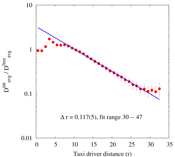
Figure 13: Ratio of interacting to free field case (cut=1).

For large taxi-driver distance $r$, we expect an exponential decay $\mathcal{D}_{\rm avg}(r)\sim\exp(-r/r_{\rm ov})$, and thus expect the ratio to decay exponentially as

$$\mathcal{D}_{\rm avg}^{\rm int}(r)/\mathcal{D}_{\rm avg}^{\rm free}(r)\sim\exp(-r/\Delta r)$$ (5)

where

$$\frac{1}{\Delta r}\equiv\left(\frac{1}{r_{\rm int}}-\frac{1}{r_{\rm free}}\right)$$ (6)

The graph is fit quite nicely with a long straight line giving a value $\Delta r=0.117(5)$. Notice that a positive value indicates that $r_{\rm int}<r_{\rm free}$. Initially, this was not expected from preliminary mobility-edge arguments [2]. But it is now acknowledged that the connection between mobility edge and overlap range is severed already in the free-field case [15]. Furthermore, a crude heuristic argument in support of the observation can be made. To wit, regard $D(x,y)$ as a sum of contributions from various paths of links connecting source $y$ to sink $x$. In the free case, the product of these links is the identity. In the interacting case, it is a path-dependent matrix with norm less than one. Then one would expect ${\mathcal{D}}^{int}(r)<{\mathcal{D}}^{free}(r)$ for each $r$. If each decays exponentially at large $r$, then one cannot have $r_{\rm int}>r_{\rm free}$ without contradiction.

2 Scaling

At Lattice 2004, Davies et al. [16] collected world data to demonstrate that different quenched quark formulations could have a consistent continuum limit.

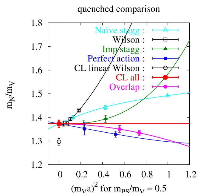
Figure 14: “Aoki” plot for various quenched data, as obtained from [16]. Our data (solid circles) are labeled “overlap”.

The conclusion, as illustrated in Fig. 14, is that they could. But we emphasize that the constrained fit demanded that there exist a global continuum limit (by design). Furthermore, the global continuum limit differed substantially from the continuum limit obtained solely from the Wilson formulation where the discretization errors are the largest. The lesson learned is that with large discretization errors, it is quite possible to be misled when extrapolating to the continuum limit, even with high statistics and many lattice spacings. It is important to seek a formulation with very small discretization errors to be able to trust the continuum extrapolation.

Here we add our data “overlap” (solid circles in Fig. 14) to the global quenched spectrum data and find that of all the formulations, its discretization errors are smallest, allowing for viable computation at surprisingly coarse lattice spacing.

As another example of the efficacy of the overlap formulation, we made a non-perturbative computation [17] of the renormalization constants of composite operators on the $16^{3}\times 28$ lattice using the regularization independent scheme.

We found that the relations $Z_{A}=Z_{V}$ and $Z_{S}=Z_{P}$ agree well (within 1%) above the renormalization point $p=1.6\,{\rm GeV}$. The $m\Lambda_{\rm QCD}a^{2}$ and $(ma)^{2}$ corrections of the renormalization are small; the mass dependence is less than about 3% up to $ma=0.6$.

3 Conclusions

It is viable to simulate quenched overlap fermions at surprisingly coarse lattice spacing. Locality is well under control; the range (characteristic exponential decay length) is about one lattice unit (of Euclidean distance, or about two lattice units of Taxi-driver distance) for lattice spacing as coarse as $0.20\,{\rm fm}$ ($f_{\pi}$ scale), such as that used in [3], and trends to zero (in physical units) in the continuum limit. Scaling is excellent; the Aoki plot is almost flat up to $0.20\,{\rm fm}$. The overlap fermion outperforms the other formulations, that is, discretization errors are the smallest for overlap. Non-perturbative renormalization of operators show little mass dependence [17]; e.g. less than about 3% up to $ma=0.6$ for the renormalization factors.

4 Acknowledgments

This work is supported in part by the U.S. Department of Energy under grant DE-FG05-84ER40154. The work of NM is supported by U.S. DOE Contract No. DE-AC05-06OR23177, under which Jefferson Science Associates, LLC operates Jefferson Lab.

References

- [1] P. Hernandez, K. Jansen, and M. Luscher, Nucl. Phys. B552, 363 (1999), hep-lat/9808010.
- [2] M. Golterman, Y. Shamir, and B. Svetitsky, Phys. Rev. D72, 034501 (2005), hep-lat/0503037.
- [3] Y. Chen, S.J. Dong, T. Draper, I. Horvath, F.X. Lee, K.F. Liu, N. Mathur, and J.B. Zhang, Phys. Rev. D70, 034502 (2004), hep-lat/0304005.
- [4] T. Draper, N. Mathur, J. Zhang, A. Alexandru, Y. Chen, S.-J. Dong, I. Horvath, F.X. Lee, and S. Tamhankar, PoS LAT2005, 120 (2006), hep-lat/0510075.
- [5] S. Durr, C. Hoelbling, and U. Wenger, JHEP 09, 030 (2005), hep-lat/0506027.
- [6] Y. Iwasaki, Nucl. Phys. B258, 141 (1985).
- [7] R. Sommer, Nucl. Phys. B411, 839 (1994), hep-lat/9310022.
- [8] H. Neuberger, Phys. Lett. B417, 141 (1998), hep-lat/9707022.
- [9] R. Narayanan and H. Neuberger, Nucl. Phys. B443, 305 (1995), hep-th/9411108.
- [10] C. Alexandrou, E. Follana, H. Panagopoulos, and E. Vicari, Nucl. Phys. B580, 394 (2000), hep-lat/0002010.
- [11] S. Capitani, Nucl. Phys. B592, 183 (2001), hep-lat/0005008.
- [12] P. Hernandez, K. Jansen, L. Lellouch, and H. Wittig, JHEP 07, 018 (2001), hep-lat/0106011.
- [13] S.J. Dong, T. Draper, I. Horvath, F.X. Lee, K.F. Liu, J.B. Zhang, Phys. Rev. D65, 054507 (2002), hep-lat/0108020.
- [14] C. W. Bernard, T. Draper, and K. Olynyk, Phys. Rev. D27, 227 (1983).
- [15] Y. Shamir, private communication.
- [16] C. T. H. Davies, G. P. Lepage, F. Niedermayer, and D. Toussaint, Nucl. Phys. Proc. Suppl. 140, 261 (2005), hep-lat/0409039.
- [17] J.B. Zhang, N. Mathur, S.J. Dong, T. Draper, I. Horvath, F.X. Lee, D.B. Leinweber, K.F. Liu, A.G. Williams, Phys. Rev. D72, 114509 (2005), hep-lat/0507022.