Thermodynamics of (2+1)-flavor QCD

Abstract

BNL-NT-06/31

We report on the status of our QCD thermodynamics project. It is performed on the QCDOC machine at Brookhaven National Laboratory and the APEnext machine at Bielefeld University. Using a 2+1 flavor formulation of QCD at almost realistic quark masses we calculated several thermodynamical quantities. In this proceeding we show the susceptibilites of the chiral condensate and the Polyakov loop, the static quark potential and the spatial string tension.

1 Introduction and Lattice Setup

The calculation of QCD thermodynamics from first principle is important for various research areas such as Heavy Ion Phenomenology, Cosmology and Astrophysics. Lattice QCD enables us to carry out such calculations. Especially for HIC phenomenology it is mandatory to improve estimates on some basic thermodynamic quantities which have been obtained in previous lattice calculations. Since thermodynamics of lattice QCD requires huge computational resources, it is difficult to perform an ideal simulation. Recent studies tell us that quark masses and the number of flavors strongly affect thermodynamic quantities [1]. Reliable continuum extrapolations are of tremendous importance as well [2]. Therefore, it is our goal to study QCD thermodynamics with almost realistic quark masses on the QCDOC machine at Brookhaven National Laboratory and the APEnext machine at Bielefeld University. The calculation is performed with $N_{f}=2+1$, which means 2 degenerate light quarks and one heavier quark on lattices with $N_{t}=4$ and 6. The lightest quark masses of our simulation yields a pion mass of about 150 MeV and kaon mass of about 500 MeV.

For such calculations we adopt the p4fat3 quark action, which is an improved Staggered quark action [3], with a tree-level improved Symanzik gauge action. By using the p4fat3 action, the free quark dispersion relation has the continuum form up to $O(p^{4})$, and taste symmetry breaking is suppressed by a 3-link fattening term. The action also improves bulk thermodynamical quantities in the high temperature limit [3]. The improvements are essential to control the continuum extrapolation on rather coarse lattices, i.e. $N_{t}=4$ and 6. The gauge ensembles are generated by an exact RHMC algorithm [4].

As a status report of the project, in this proceeding, we present several thermodynamics quantities, which are susceptibilities of the light and strange quark chiral condensate, the Polyakov loop susceptibility, the static quark potential, and the spatial string tension. The details of the critical temperature calculation are given in our recent paper [5].

2 Order Parameters and Susceptibilities

To investigate the QCD critical temperature and phase diagram, order parameter of the QCD transition are indispensable. In the chiral limit the chiral condensate $\langle\bar{\psi}\psi\rangle$ is the order parameter for the spontaneous chiral symmetry breaking of QCD. On the other hand in the heavy quark limit the Polyakov loop $\langle L\rangle$ is the order parameter of the deconfinement phase transition. For finite quark masses, these observables remain good indicators for the (pseudo) critical point. Especially their susceptibilities are useful to determine the critical coupling $\beta_{c}$ in numerical simulations.

Figure 1 shows the susceptibilities of the chiral condensate and the Polyakov loop. Their peak positions define the point of most drastic change of each order parameters, i.e. the (pseudo) critical point of the QCD transition. The results are interpolated in the coupling $\beta$ by using the multi-histogram re-weighting technique [6].

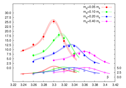
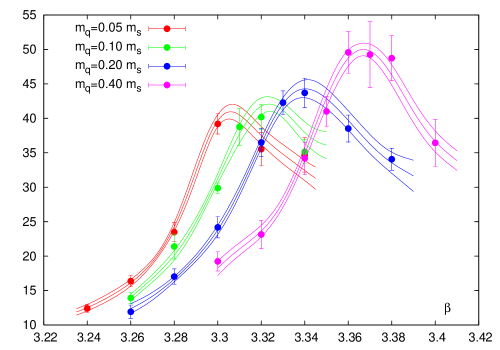
Figure 1: The susceptibility of the chiral condensate (left) and the susceptibility of the Polyakov loop (right) on $8^{3}\times 4$ lattices. In the left panel filled and open symbols are results for light and strange quarks, respectively. The lines are calculated by the multi-histogram re-weighting technique.

The strength of the transition decreases with increasing quark masses, this is reflected in the decreasing peak height of the chiral susceptibilities. We calculate these susceptibilities on lattices with aspect ratios of $N_{s}/N_{t}=2$ and 4. Since we see a rather small volume dependence the results suggest that the transition is in fact not a true phase transition in the thermodynamic sense but a rapid crossover. The peak position of the chiral and Polyakov loop susceptibilities are almost identical, i.e. the chiral and deconfinement transition occur at almost the same temperature. The discrepancy between the peak positions shrinks with increasing volume.

3 Scale Setting and the Heavy Quark Potential

The lattice scale is determined from the heavy quark potential $V(r)$ which is extracted from Wilson loops. The Wilson loop expectation values are calculated on $16^{3}\times 32$ lattices with APE smearing in spatial direction. The spatial path in a loop is determined by the Bresenham algorithm [8]. We calculate the string tension, $\sigma$ and Sommer scale $r_{0}$, which is defined [7] as the distance where the corresponding force of the static quark potential matches a certain value suggested by phenomenology: $r^{2}\frac{\partial V}{\partial r}\mid_{r=r_{0}}=1.65$. To remove short range lattice artifacts we use the improved distance, $r_{imp}$, which is defined as

$$\frac{1}{4\pi r_{imp}}\equiv\int\frac{d^{3}k}{(2\pi)^{3}}\frac{e^{ikr}}{4\sum_{i}(\sin^{2}{\frac{k_{i}}{2}})+\frac{1}{3}\sin^{4}{\frac{k_{i}}{2}}}.$$ (1)

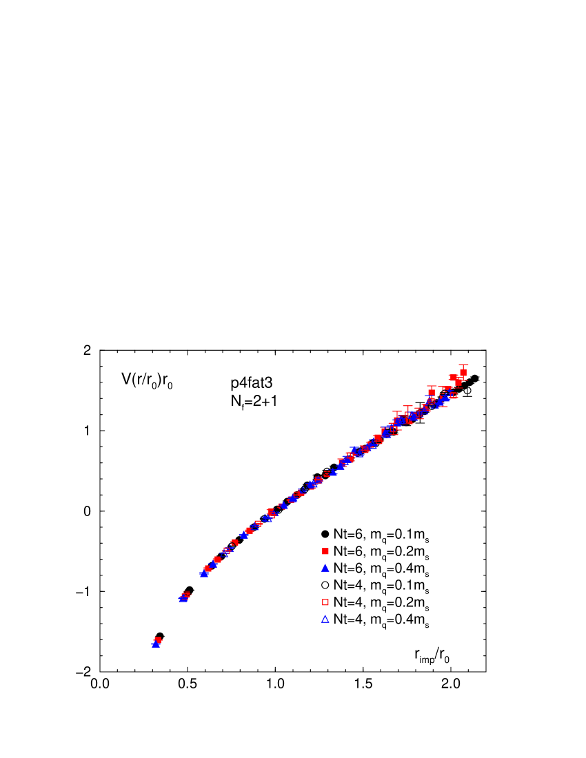
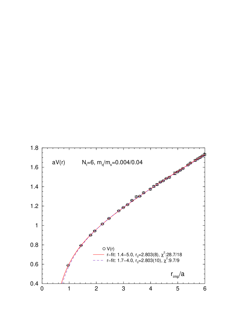
Figure 2: Heavy quark potentials scaled by $r_{0}$ for various cut-offs and quark masses (left) and the fit-range dependence of $r_{0}$ (right). The latter shows the result for $N_{t}=4,m_{q}/m_{s}=0.026/0.065$ and fits with the 3-params. fit-form.

In our lattice setup, we find almost no mass and cutoff dependence in the potential scaled by $r_{0}$ at $N_{\tau}=4$ and 6 (Fig.2(left)). As discussed in previous studies [9], we also find no string breaking effects even at large $r$.

To estimate systematic uncertainties of the potential fit, we performed several types of fits, e.g. different fit-ranges in $r$ (see Fig.2(right)) and fit-forms (3 & 4 params. fits),

$$V(r)=C+\frac{\alpha}{r_{imp}}+\sigma r_{imp},~{}~{}~{}V(r)=C+\frac{\alpha}{r}+\sigma r+d(\frac{\alpha}{r_{imp}}-\frac{\alpha}{r}).$$ (2)

The differences in the mean values of the fits are evaluated as a systematic uncertainty of the scale setting. From a combined quark mass and cut off extrapolation of $r_{0}T_{c}\equiv(r_{0}/a)(aT_{c})$ we finally obtain a critical temperature of $T_{c}=192(7)(4)$ MeV at the physical point [5]. Here we used $r_{0}=0.469$ fm to set the scale. The first error summarizes all statistical and systematic errors on $r_{0}$ and the critical couplings $\beta_{c}$ and the second error reflects the remaining uncertainties in the extrapolation.

4 Spatial String Tension

Let us now discuss the calculation of the spatial string tension which is important to verify the theoretical concept of dimensional reduction at high temperatures. The spatial string tension is extracted from the spatial static quark “potential” (from spatial Wilson loops). We use the same analysis technique as for the usual (temporal) static quark potential.

At high temperature, the spatial string tension $\sigma_{s}(T)$ is expected to behave like

$$\sqrt{\sigma_{s}(T)} = cg^{2}(T)T.$$ (3)

Here $g^{2}(T)$ is the temperature dependent coupling constant from the 2-loop RG equation,

$$g^{-2}(T) = 2b_{0}\ln{\frac{T}{\Lambda_{\sigma}}}+\frac{b_{1}}{b_{0}}\ln{\left(2\ln{\frac{T}{\Lambda_{\sigma}}}\right)}.$$ (4)

If dimensional reduction works, the parameter“$c$” should be equal to the 3-dimensional string tension and should be flavor independent.

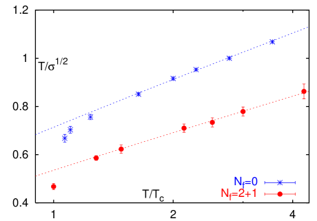
Figure 3: Temperature dependence of the spatial string tension for $N_{f}=0$ [10] and $N_{f}=2+1$. Both dotted lines are fits with Eq. 3. Note, that the scale on the horizontal axis is logarithmic.

Our 2+1 flavor result yields $c=0.587(41)$ and $\Lambda_{\sigma}/T_{c}=0.114(27)$, obtained by a fit with Eq. 3. On the other hand, we plot in Fig.3 also the quenched result [10] which gives $c=0.566(13)$ and $\Lambda_{\sigma}/T_{c}=0.104(9)$. We thus find that the parameter “c” is – within statistical errors – independent on the number of dynamical flavors and that dimensional reduction works well even for $T=2T_{c}$. This analysis can and will be refined in the future by taking into account higher order corrections to Eq. 3 [11].

References

- [1] F. Karsch, E. Laermann and A. Peikert, Nucl. Phys. B 605, 579 (2001).
- [2] A. Ali Khan et al. [CP-PACS collaboration], Phys. Rev. D 64, 074510 (2001).
- [3] U. M. Heller, F. Karsch and B. Sturm, Phys. Rev. D 60, 114502 (1999).
- [4] M. A. Clark, A. D. Kennedy and Z. Sroczynski, Nucl. Phys. Proc. Suppl. 140, 835 (2005).
- [5] M. Cheng et al., arXiv:hep-lat/0608013, to appear in Phys. Rev. D.
- [6] A. M. Ferrenberg and R. H. Swendsen, Phys. Rev. Lett. 61 (1988) 2635.
- [7] M. Guagnelli, R. Sommer and H. Wittig, Nucl. Phys. B 535, 389 (1998).
- [8] B. Bolder et al., Phys. Rev. D 63, 074504 (2001).
- [9] S. Aoki et al. [CP-PACS Collaboration], Phys. Rev. D 60, 114508 (1999).
- [10] G. Boyd et al., Nucl. Phys. B 469, 419 (1996).
- [11] Y. Schröder and M. Laine, PoS LAT2005, 180 (2006) [arXiv:hep-lat/0509104].