Direct numerical computation of disorder parameters

Abstract

In the framework of various statistical models as well as of mechanisms for color confinement, disorder parameters can be developed which are generally expressed as ratios of partition functions and whose numerical determination is usually challenging. We develop an efficient method for their computation and apply it to the study of dual superconductivity in 4$d$ compact $U(1)$ gauge theory.

I Introduction

Order-disorder transitions are common to a wide class of models in Statistical Mechanics and Quantum Field Theory, the Ising model being a prototype Kramers:1941kn ; Kadanoff:1970kz . In those models, one phase is characterized by the condensation of dual topological excitations which spontaneously breaks a dual symmetry, and correlation functions of those excitations can serve as disorder parameters for the transition: in general they are non local in terms of the original variables, so that their numerical study can be challenging. The difficulty becomes evident when the correlation functions are expressed as ratios of partition functions.

Relevant examples are encountered when studying color confinement in QCD: that is usually believed to be related to the condensation of some topological excitations and models can be constructed accordingly, which place the confinement-deconfinement transition into the more general scenario of order-disorder transitions. One appealing model is based on dual superconductivity of the QCD vacuum and relates confinement to the breaking of an abelian dual symmetry induced by the condensation of magnetic monopoles thooft75 ; mandelstam ; parisi . The possibility to define disorder parameters in this scenario has been studied since a long time Frohlich:1986-87 ; fro ; mar ; del ; DiGiacomo:1997sm . One parameter has been developed by the Pisa group and is the expectation value of an operator $\mu$ which creates a magnetic monopole; $\langle\mu\rangle$ has been shown to be a good parameter for confinement in $U(1)$ DiGiacomo:1997sm , in pure Yang-Mills theories PaperI ; PaperIII and in full QCD full1 ; full2 ; similar parameters have been developed both in gauge theories moscow ; bari ; marchetti ; bari2 and in statistical models xymodel ; heisenberg ; ising . The operator $\mu$ is expressible as the exponential of the integral over a time slice, $\mu=\exp(-\beta\Delta S)$ (see later for details), so that its expectation value can be rewritten (we consider a pure gauge theory as an example) as

$$\langle\mu\rangle=\frac{\int\left({\cal D}U\right)e^{-\beta(S+\Delta S)}}{\int\left({\cal D}U\right)e^{-\beta S}}=\frac{\int\left({\cal D}U\right)e^{-\beta\tilde{S}}}{\int\left({\cal D}U\right)e^{-\beta S}}\equiv\frac{\tilde{Z}}{Z}\;,$$ (1)

where the functional integration is over the gauge link variables, $S$ is the euclidean action of the theory and $\beta$ is the inverse gauge coupling. The difficulty involved in its numerical computation stems from the poor overlap among the two statistical distributions corresponding to the partition functions $Z$ and $\tilde{Z}$: configurations which give significant contributions to $\tilde{Z}$ are instead extremely rare in the original ensemble corresponding to $Z$, so that they are very badly sampled in a Monte Carlo simulation. The problem worsens rapidly when increasing the spatial volume, making a determination of $\langle\mu\rangle$ hardly feasible. One way out is to evaluate susceptibilities of $\langle\mu\rangle$, like:

$$\rho=\frac{d}{d\beta}\ln\langle\mu\rangle=\langle S\rangle_{S}-\langle\tilde{S}\rangle_{\tilde{S}}\;,$$ (2)

from which the disorder parameter can eventually be reconstructed as follows

$$\langle\mu\rangle=\exp\left({\,\int_{0}^{\beta}\rho(\beta^{\prime}){\rm d}\beta^{\prime}}\right)\;\,.$$ (3)

While that is enough to test $\langle\mu\rangle$ as a parameter for confinement, a direct determination could be useful in contexts like the study of its correlation functions DiGiacomo:1997sm ; u1mass ; su2mass .

The problem of dealing with extremely rare configurations can be approached using the idea of generalized ensembles umbrella ; multicanonical ; tempering . In that framework we propose a new method for a direct computation of $\langle\mu\rangle$, which is inspired by analogous techniques used for the study of the ’t Hooft loop thooftloop . We describe the method for the case of the $4d$ compact $U(1)$ gauge theory in the Wilson formulation, but it is applicable to the study of disorder parameters in a wide class of analogous problems.

II The method

The partition function of the model is defined, in the Wilson formulation, as follows

$$Z(\beta)=\int[d\theta]e^{\,-\beta S}\,$$ (4)

$$S=\sum_{\overrightarrow{x,}t,(\mu\nu)}\left(1-\cos(\theta_{\mu\nu}(\vec{x},t)\right)\,.$$ (5)

where the integration is over the link variables (phases in $U(1)$) and $\theta_{\mu\nu}(\vec{x},t)$ is the plaquette in the $\mu\nu$ plane sitting at lattice site $(\vec{x},t)$. The model has a critical point at $\beta_{c}\simeq 1.01$, which is believed to be weak first order and separates a disordered phase ($\beta<\beta_{c}$), with condensation of magnetic monopoles and confinement of electric charges, from a Coulomb phase where magnetic charge condensation disappears.

The magnetically charged operator $\mu(\vec{y},t_{0})$, whose expectation value detects dual superconductivity, creates a monopole in $\vec{y}$ at time $t_{0}$ by shifting the quantum gauge fields by the classical vector potential of a monopole, $\vec{b}(\vec{x}-\vec{y})$, and can be written (see Ref. DiGiacomo:1997sm for details) as

$$\mu(\vec{y},t_{0})=\exp\left[i\frac{1}{e}\int\text{{{d}}}^{3}x\hskip 2.5pt\vec{E}(\vec{x},t_{0})\vec{b}(\vec{x}-\vec{y})\right]\,,$$ (6)

with the electric field $\vec{E}(\vec{x},t_{0})$ being the momentum conjugate to the quantum vector potential. It can be discretized on the lattice as follows:

$$\mu=e^{\beta\sum_{\vec{x},i}\left(\cos\left(\theta_{0i}(\vec{x},t_{0})-b_{i}(\vec{x}-\vec{y})\right)-\cos(\theta_{0i}(\vec{x},t_{0}))\right)}\equiv e^{-\beta\Delta S}\;,$$ (7)

where $\theta_{0i}$ are the phases of the temporal plaquettes, corresponding to the electric field in the (naïve) continuum limit. If we define the modified action

$$\tilde{S}=\sum_{\overrightarrow{x,}t\neq t_{0},(\mu\nu)}\left(1-\cos(\theta_{\mu\nu})\right)$$ (8)

$$+ \sum_{\vec{x},i}\left(1-\cos(\theta_{0i}(\vec{x},t_{0})-b_{i}(\vec{x}-\vec{y}))\right)=S+\Delta S\;$$

which differs from $S$ only on the timeslice where the monopole has been created, we can write

$$\langle\mu(\vec{y},t)\rangle=\tilde{Z}(\beta)/Z(\beta)\,;$$ (9)

$$\tilde{Z}(\beta)=\int[d\theta]\exp(-\beta\tilde{S})\,.$$ (10)

Measuring $\langle\mu(\vec{y},t)\rangle$ in a Monte Carlo (MC) simulation is very difficult DiGiacomo:1997sm : $\mu$ gets significant contributions only on those configurations having very small statistical weight (which are poorly sampled in a finite MC simulation). The difficulty increases with the system size as the two distributions corresponding to $Z$ and $\tilde{Z}$ shrink towards non overlapping delta functions in the configuration space. Our proposal is to determine the ratio in Eq. (9) by using intermediate distribution functions having a reasonable overlap with both statistical ensembles corresponding to $Z$ and $\tilde{Z}$: our method has many similarities with strategies adopted in the computation of analogous order parameters kovacs ; rebbi ; deforc ; helicity . As a first step we rewrite the ratio as the product of $N$ distinct ratios:

$$\frac{\tilde{Z}}{Z}=\frac{Z_{N}}{Z_{N-1}}\,\frac{Z_{N-1}}{Z_{N-2}}\,\dots\,\frac{Z_{1}}{Z_{0}}\;,$$ (11)

where $Z_{N}\equiv\tilde{Z}$, $Z_{0}\equiv Z$ and $Z_{k}$ is defined in terms of an action $S_{k}$ which is an interpolation between $S$ and $\tilde{S}$:

$$Z_{k}\equiv\int[d\theta]e^{-\beta{S_{k}}}\,;$$ (12)

$$S_{k}\equiv\frac{N-k}{N}S+\frac{k}{N}\tilde{S}\,.$$ (13)

The idea is to compute each single ratio by a different Monte Carlo simulation: the difficulty of dealing with $N$ simulations should be greatly compensated by the increased overlap in the distributions corresponding to each couple of partition functions, leading to a benefit which increases exponentially with $N$. As a second step to further improve the overlap, we compute each single ratio on the r.h.s. of Eq. (11) using an intermediate distribution:

$$\frac{Z_{k+1}}{Z_{k}}=\frac{\left\langle\exp\left(-\beta\Delta{S}/2N\right)\right\rangle_{k+1/2}}{\left\langle\exp\left(\beta\Delta S/2N\right)\right\rangle_{k+1/2}}\;,$$ (14)

where each expectation value is computed with the action

$$S_{k+1/2}\equiv\left(1-(k+1/2)/N\right)\,S+\left((k+1/2)/N\right)\,\tilde{S}.$$ (15)

Since both expectation values in Eq. (14) are computed with the same MC simulation, we make use of a jackknife analysis to get a reliable error on $Z_{k+1}/Z_{k}$. The final uncertainty on $\tilde{Z}/Z$ is then obtained by standard error propagation since each single ratio on the r.h.s. of Eq. (11) is obtained by an independent MC simulation.

Our technique of rewriting the ratio $\tilde{Z}/Z$ as a product of intermediate ratios resembles very closely the well known snake algorithm deforc as well as other algorithms inspired by it, like that used for the computation of the helicity modulus helicity . However it differs from previous algorithms in the choice of the intermediate partition functions, which in our case is not related to the details of the model, so that it can be applied without modifications to a wider class of problems in Lattice Field Theory and Statistical Mechanics.

Regarding the choice of boundary conditions (b.c.), we do it in a consistent equal way for all the partition functions in Eq. (11). We make use of both periodic and free b.c. in the spatial directions: while one could expect a substantial difference in presence of a magnetic charge, we will show that, in the phase where $\langle\mu\rangle\neq 0$, the two choices lead to the same thermodynamical limit; that is expected since in that phase the vacuum does not have a well defined magnetic charge and a monopole is completely screened. As for the temporal direction, a consistent usual choice for $\langle\mu\rangle$ DiGiacomo:1997sm is that of periodic b.c. for $Z$ and $C^{*}$ b.c. for $\tilde{Z}$; in particular $C^{*}$ boundary conditions, which corresponds to performing a charge conjugation transformation on gauge fields when crossing the time boundary, are taken so as to annihilate the monopole after one loop around the periodic time direction, avoiding in this way that it propagates an indefinite number of times. However we do not keep that choice, since it would lead to intermediate actions with inconsistent mixed b.c.; instead we adopt either free or periodic b.c. for both $Z$ and $\tilde{Z}$ also in the time direction, showing again that the choice is inessential when $\langle\mu\rangle\neq 0$.

III Numerical results

As a first test we compare the naïve computation of $\langle\mu\rangle$, i.e. performed with a single MC simulation using the Wilson action $S$, with our method for $N=1$: we use a $4^{4}$ lattice with free b.c. at $\beta=0.8$ and $10^{7}$ measurements for both cases, obtaining $\langle\mu\rangle=1.14(18)$ with the naïve computation and $\langle\mu\rangle=0.868(3)$ with our method. Apart from the strongly reduced error, much is learned by looking at the distributions of the observables $\exp(-\beta\Delta S)_{S}$ and $\exp(\pm\beta\Delta S/2)_{(S+\tilde{S})/2}$ (the subscript indicates the action used for sampling) used in the computation (see Eq. 14). In Fig. 1 we plot, for each fixed observable $O$, the distribution of the logarithm of $O$ times the observable itself (we choose the logarithm for graphical convenience) as a function of $\log O$, so that the integral of each curve gives the expectation value of the relative observable. As it is clear, for $\langle\exp(-\beta\Delta S)\rangle_{S}$ most of the contribution comes from a region which is badly sampled: on larger lattices the problem worsens rapidly and a naïve determination of $\langle\mu\rangle$ is unfeasible. The improvement obtained with our method is apparent already for $N=1$.

In Fig. 2 we show a determination of $\langle\mu\rangle$ for several values of $N$ on a lattice $16^{4}$ with free b.c. at $\beta=0.8$: for each determination a comparable whole statistics of $N\times N_{\rm meas}=3.2\cdot 10^{5}$ measurements has been used, so that the error on $\langle\mu\rangle$ is an indication of the efficiency as a function of $N$; in Fig. 3 we report the intermediate ratios $Z_{k+1}/Z_{k}$ (see Eq. 11) used for each measurement. While the intermediate ratios are strongly dependent on $N$, $\langle\mu\rangle$ is not, thus confirming the absence of uncontrolled systematic errors. The statistical error rapidly changes for small values of $N$, but then stabilizes, indicating that a value $N\sim O(10)$ saturates the improvement.

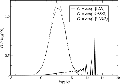
Figure 1: For each observable $O$ involved in the computation on the $4^{4}$ lattice at $\beta=0.8$, we plot $O$ times the distribution of $\log O$ as a function of $\log O$: the integral under each curve gives $\langle O\rangle$.

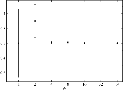
Figure 2: Determination of $\langle\mu\rangle$ on a lattice $16^{4}$ with free b.c. at $\beta=0.8$ as a function of $N$.

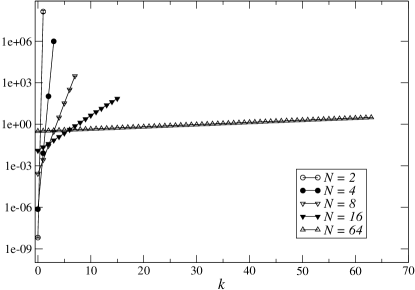
Figure 3: Intermediate ratios $Z_{k+1}/Z_{k}$ used for the determinations reported in Fig. 2.

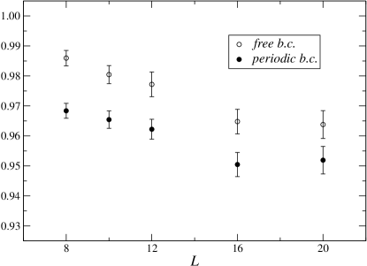
Figure 4: $\langle\mu\rangle$ at $\beta=0.5$ as a function of the lattice size $L$ determined with both free and periodic b.c.

As an application of our method we analyse some relevant features of the disorder parameter, starting with a study of its thermodynamical limit in the confined phase. In Fig. 4 we show $\langle\mu\rangle$ determined with both free and periodic b.c. at $\beta=0.5$ as a function of the lattice size $L$. A fit according to $\langle\mu\rangle=A+B/L$ gives $A=0.945(6)$ and $B=0.31(6)$ with free b.c. ($\tilde{\chi}^{2}=0.5$) and $A=0.940(6)$ and $B=0.2(6)$ with periodic b.c. ($\tilde{\chi}^{2}=0.8$). In both cases $\langle\mu\rangle$ has a well defined thermodynamical limit, which does not depend (within numerical errors) on the b.c. chosen: that is expected in the phase where magnetic charge is completely screened. We stress that, contrary to what may happen with other parameters helicity , we do not expect exactly $\langle\mu\rangle=1$ in the confined phase: indeed any non-zero value of the disorder parameter ensures the breaking of the magnetic symmetry, hence dual superconductivity.

A further confirmation of screening comes from the study of cluster property in the correlation functions. In Table 1 we report the values measured for various temporal and spatial correlators of $\mu$ using periodic b.c., together with their second and fourth powers. In this way we compare, for instance, the value of $\langle\mu\rangle^{2}$ (first row, second column) with that of the two point function $\langle\bar{\mu}\mu\rangle$ at large distances (first column, second row), or $\langle\mu\rangle^{4}$ with the four point function, and so on: the compared quantities should approach each other (exponentially in the extension of the higher order correlator) if cluster property is obeyed. This is nicely verified, within errors, from the data reported in the Table.

	$\mathcal{O}$	$\mathcal{O}^{2}$	$\mathcal{O}^{4}$
$\langle\mu(\vec{0},0)\rangle$	0.439(12)	0.193(11)	0.037(4)
$\langle\bar{\mu}(\vec{0},t)\mu(\vec{0},0)\rangle$	0.182(7)	0.033(3)
$\langle\bar{\mu}(\vec{z},0)\mu(\vec{0},0)\rangle$	0.183(12)	0.033(4)
$\langle\bar{\mu}(\vec{z},0)\bar{\mu}(\vec{0},t)\mu(\vec{z},t)\mu(\vec{0},0)\rangle$	0.037(6)

Table 1: Determination at $\beta=0.8$ on a $16^{4}$ lattice of $\langle\mu\rangle$, of its spatial and temporal 2-point function (second and third row) and of its mixed 4-point function (last row), with $t=8$ and $\vec{z}=(0,0,8)$. The measured correlator is reported in the first column, indicated generically with $\mathcal{O}$, while in the second and third column (indicated with $\mathcal{O}^{2}$ and $\mathcal{O}^{4}$) we report respectively the second and fourth power of the correlator, which are used to test cluster property on the higher order correlators reported in lower rows. Within errors all measurements are compatible with the hypothesis that the correlators are  already in  their asymptotic regime governed by cluster property.

Figure 5: $\langle\mu\rangle$ at $\beta=1.1$ as a function of the lattice size $L$ determined with both free and periodic b.c.

Results are quite different in the deconfined phase. In Fig. 5 we show $\langle\mu\rangle$ as a function of $L$ at $\beta=1.1$: the determinations with free and periodic b.c. differ from each other, both going to zero exponentially with the lattice size $L$. This is the correct expected behavior in the phase with magnetic charge superselection DiGiacomo:1997sm ; supersel .

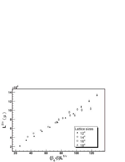
Figure 6: F.s.s. analysis of $\langle\mu\rangle$ around the phase transition

Finally we consider the critical behaviour of the disorder parameter close to the phase transition, where $\langle\mu\rangle\simeq\tau^{\delta}$ ($\tau$ is the reduced temperature). That translates in the following finite size scaling (f.s.s.) behaviour

$$\langle\mu\rangle=L^{-\frac{\delta}{\nu}}\phi\left((\beta_{c}-\beta)L^{1/\nu}\right)$$ (16)

where $\phi$ is a scaling function. To test this ansätz we have determined $\langle\mu\rangle$ close to the phase transition on several different lattice sizes. Fixing the known value of $\beta_{c}=1.011$ and $\nu=1/d=0.25$ as appropriate for a weak first order transition, we obtain a reasonable scaling with $\delta\sim 2.3$: the quality of our f.s.s. analysis is shown in Fig. 6.

IV Conclusions

We have proposed a new technique for the computation of disorder parameters and applied it to the study of the parameter for dual superconductivity in 4$d$ compact U(1) gauge theory. Our method is inspired by methods used for the study of the ’t Hooft loop deforc .

We have determined some relevant features of $\langle\mu\rangle$ both in the confined and in the Coulomb phase. A careful analysis of its critical properties could help in clarifying the nature of the phase transition at zero as well as at finite temperature finiteU1-berg ; finiteU1-defor : to that aim also a direct comparison with analogous order parameters developed for $U(1)$ bari2 ; helicity will be particularly useful.

Our method can be placed in the more general framework of techniques based on the idea of generalized ensembles umbrella ; multicanonical ; tempering : in that respect, it has the advantage to provide a recipe which can be easily applied, with none or few modifications, to a wide class of problems. Among others we will consider in the future the study of order-disorder transitions in statistical models and dual superconductivity in non Abelian gauge theories. Another benefit of our proposal is that it leaves room for considerable further improvement: for instance it could be possible to choose a more general non linear interpolation between the two actions $S$ and $\tilde{S}$, differently from what has been done in Eq. (13), so as to concentrate the numerical effort on those intermediate ensembles where the statistical distribution is changing more rapidly.

- (1) H.A. Kramers and G.H. Wannier, Phys. Rev. 60, 252 (1941).
- (2) L.P. Kadanoff and H. Ceva, Phys. Rev. B 3, 3918 (1971).
- (3) G. ’t Hooft, in “High Energy Physics”, EPS International Conference, Palermo 1975, ed. A. Zichichi.
- (4) S. Mandelstam, Phys. Rept. 23, 245 (1976).
- (5) G. Parisi, Phys. Lett. B 60, 93 (1975).
- (6) J. Frohlich and P.A. Marchetti, Europhys. Lett. 2, 933 (1986); Commun. Math. Phys. 112, 343 (1987).
- (7) J. Frohlich and T. Spencer, Commun. Math. Phys. 83, 411 (1982).
- (8) E. C. Marino, B. Schroer and J. A. Swieca, Nucl. Phys. B200, 473 (1982).
- (9) L. Del Debbio, A. Di Giacomo and G. Paffuti, Phys. Lett. B 349, 513 (1995).
- (10) A. Di Giacomo and G. Paffuti, Phys. Rev. D 56, 6816 (1997).
- (11) A. Di Giacomo, B. Lucini, L. Montesi and G. Paffuti, Phys. Rev. D 61, 034503 (2000); Phys. Rev. D 61, 034504 (2000).
- (12) J. M. Carmona, M. D’Elia, A. Di Giacomo, B. Lucini and G. Paffuti, Phys. Rev. D 64, 114507 (2001).
- (13) J. M. Carmona, M. D’Elia, L. Del Debbio, A. Di Giacomo, B. Lucini and G. Paffuti, Phys. Rev. D 66, 011503 (2002).
- (14) M. D’Elia, A. Di Giacomo, B. Lucini, C. Pica and G. Paffuti, Phys. Rev. D 71, 114502 (2005).
- (15) M.N. Chernodub, M.I. Polikarpov and A.I. Veselov, Phys. Lett. B 399, 267 (1997).
- (16) P. Cea and L. Cosmai, JHEP 0111, 064 (2001).
- (17) J. Frohlich and P.A. Marchetti, Phys. Rev. D 64, 014505 (2001).
- (18) P. Cea, L. Cosmai and M. D’Elia, JHEP 0402, 018 (2004).
- (19) G. Di Cecio, A. Di Giacomo, G. Paffuti and M. Trigiante, Nucl. Phys. B489, 739 (1997).
- (20) A. Di Giacomo, D. Martelli and G. Paffuti, Phys. Rev. D 60, 094511 (1999).
- (21) J. M. Carmona, A. Di Giacomo and B. Lucini, Phys. Lett. B 485, 126 (2000).
- (22) G. ’t Hooft, Nucl. Phys. B138, 1 (1978).
- (23) G. M. Torrie and J. P. Valleau, J. Comp. Phys. 23, 187 (1977).
- (24) B. A. Berg and T. Neuhaus, Phys. Lett. B 267, 249 (1991).
- (25) E. Marinari and G. Parisi, Europhys. Lett. 19, 451 (1992).
- (26) L. Tagliacozzo, Phys. Lett. B 642, 279 (2006).
- (27) A. D’Alessandro, M. D’Elia and L. Tagliacozzo, hep-lat/0607014.
- (28) T.G. Kovacs and E.T. Tomboulis, Phys. Rev. Lett. 85, 704 (2000).
- (29) C. Hoelbling, C. Rebbi and V. A. Rubakov, Phys. Rev. D 63, 034506 (2001).
- (30) Ph. de Forcrand, M. D’Elia, M. Pepe, Phys. Rev. Lett. 86, 1438 (2001).
- (31) Ph. de Forcrand and M. Vettorazzo, Nucl. Phys. B686, 85 (2004).
- (32) M. D’Elia, A. Di Giacomo and B. Lucini, Phys. Rev. D 69, 077504 (2004).
- (33) B.A. Berg and A. Bazavov, hep-lat/0605019.
- (34) M. Vettorazzo and Ph. de Forcrand, Phys. Lett. B 604, 82 (2004).