Critical Exponents for U(1) Lattice Gauge Theory at Finite Temperature

Abstract:

For compact U(1) lattice gauge theory (LGT) we have performed a finite size scaling analysis on $N_{\tau}N_{s}^{3}$ lattices for $N_{\tau}$ fixed and $N_{s}\to\infty$, approaching the phase transition from the confined phase. For $N_{\tau}=4$, 5 and 6 our data contradict the expected scenario that this transition is either first order or in the universality class of the 3d XY model. If there are no conceptional flaws in applying the argument that the Gaussian fixed point in 3d is unstable to our systems, estimates of the critical exponents $\alpha/\nu$, $\gamma/\nu$, $(1-\beta)/\nu$ and $2-\eta$ indicate the existence of a new, non-trivial renormalization group fixed point for second order phase transitions in 3d. Such a fixed point would be of importance for renormalization group theory and statistical physics.

1 Model and Simulation Statistics

This paper summarizes and extends work of Ref. [1] about pure U(1) LGT with the Wilson action. Multicanonical simulations [2] on

$$N_{\tau}\,N_{s}^{3}~{}~{}~{}{\rm lattices,}~{}~{}~{}N=N_{\tau}\,N_{s}^{3}$$ (1)

are performed with $N_{\tau}={\rm fixed},\ N_{s}\to\infty$ or $N_{\tau}=N_{s}$. The multicanonical parameters were determined using a modification of the Wang-Landau (WL) recursion [3]. A speed up by a factor of about three was achieved by implementing the biased Metropolis-Heatbath algorithm [4] for the updating instead of relying on the usual Metropolis procedure. Additional overrelaxation [5] sweeps are presently used for simulations on larger lattices.

Our statistics is summarized in table 1. The lattice sizes are collected in the first and second column. The third column contains the number of sweeps spent on the WL recursion for the multicanonical parameters. Typically the parameters are frozen after reaching $\epsilon=e^{1/20}$. Exceptions are the simulations for which the values are marked by $*$ for which $\epsilon=e^{1/22}$ was used (technical details will be published elsewhere). Column four lists our production statistics from simulations with fixed multicanonical weights. Error bars as shown in figures will be calculated using jackknife bins (e.g., chapter 2.7 of [6]) with their number given by the first value in column four, while the second value was also used for the number of equilibrium sweeps (without measurements) performed after the recursion. Columns five and six give the $\beta$ values between which our Markov process cycled. Adapting the definition of chapter 5.1 of [6] one cycle takes the process from the configuration space region at $\beta_{\min}$ to $\beta_{\max}$ and back. Each run was repeated once more, where after the first run the multicanonical parameters were estimated from its statistics. Columns seven and eight give the number of cycling events recorded during these runs. We are still producing on lattices with larger $N_{s}$ values than those listed in table 1 and are creating entire new series of $N_{s}$ values for $N_{\tau}=2,$ 3, 8 and 10. We perform finite size scaling (FSS) calculations for the critical exponents of U(1) LGT. For a review of FSS methods and scaling relations see [7]. The observables, which we calculated, and their FSS behavior are introduced in the following.

Table 1: Statistics.

$N_{\tau}$	$N_{s}$	WL	Production	$\beta_{\min}$	$\beta_{\max}$	cycles 1	cycles 2
4	4	11 592	$32\times 20$ $000$	0.8	1.2	527	594
4	5	14 234	$32\times 12$ $000$	0.8	1.2	146	172
4	6	19 546	$32\times 32$ $000$	0.9	1.1	258	364
4	8	29 935	$32\times 32$ $000$	0.95	1.05	229	217
4	10	25 499	$32\times 64$ $000$	0.97	1.03	175	317
4	12	47 379	$32\times 112$ $000$	0.98	1.03	338	360
4	14	44 879	$32\times 112$ $000$	0.99	1.02	329	322
4	16	54 623	$32\times 128$ $000$	0.99	1.02	19	219
4	18	58 107	$32\times 150$ $000$	0.994	1.014	93	259
4	22	73 874*	$64\times 100$ $000$	1.000	1.008	335	356
5	5	18 201	$32\times 12$ $000$	0.8	1.2	114	122
5	6	20 111	$32\times 36$ $000$	0.9	1.1	294	308
5	8	31 380	$32\times 40$ $000$	0.95	1.05	35	191
5	10	47 745	$32\times 72$ $000$	0.97	1.03	144	231
5	12	37 035	$32\times 112$ $000$	0.99	1.02	280	326
5	14	49 039	$32\times 112$ $000$	1.0	1.02	192	277
5	16	43 671	$32\times 160$ $000$	1.0	1.02	226	257
5	18	56 982	$32\times 180$ $000$	1.0	1.014	138	241
6	6	28 490	$32\times 40$ $000$	0.9	1.1	312	281
6	8	44 024	$32\times 40$ $000$	0.96	1.04	173	175
6	10	51 391	$32\times 72$ $000$	0.97	1.04	139	170
6	12	41 179	$32\times 128$ $000$	0.995	1.02	226	283
6	14	50 670	$32\times 128$ $000$	1.0	1.02	89	220
6	16	56 287	$32\times 160$ $000$	1.0	1.02	149	189
6	18	68 610	$32\times 180$ $000$	1.005	1.015	123	200
8	8	46 094	$32\times 40$ $000$	0.97	1.03	111	159
10	10	48 419	$32\times 96$ $000$	0.98	1.03	103	133
12	12	70 340	$32\times 112$ $000$	0.99	1.03	75	82
14	14	112 897	$32\times 128$ $000$	1.0	1.02	57	51
16	16	87 219	$32\times 160$ $000$	1.007	1.015	12	73
16	16	191 635*	$32\times 160$ $000$	1.007	1.015	48	74

For the Specific heat one has

$$C(\beta)\ =\ \frac{1}{6N}\left[\langle S^{2}\rangle-\langle S\rangle^{2}\right]_{\max}\sim N_{s}^{\alpha/\nu}\ .$$ (2)

Polyakov loops $P_{\vec{x}}$ are the products of U(1) gauge matrices along straight lines in the $N_{\tau}$ direction. The lattice average of Polyakov loops is defined by

$$P\ =\ \sum_{\vec{x}}P_{\vec{x}}\ .$$ (3)

The maxima of the susceptibility of the absolute value $|P|$ (called Polyakov loop susceptibility henceforth) scale like

$$\chi_{\max}\ =\ \frac{1}{N_{s}^{3}}\left[\langle|P|^{2}\rangle-\langle|P|\rangle^{2}\ \right]_{\max}\sim\ N_{s}^{\gamma/\nu}\,,$$ (4)

while for the maxima of the derivatives the scaling behavior

$$\chi^{\beta}_{\max}\ =\ \frac{1}{N_{s}^{3}}\left.\frac{d~{}}{d\beta}\,\langle|P|\rangle\ \right|_{\max}\sim\ N_{s}^{(1-\beta)/\nu}\,.$$ (5)

holds. Maxima of structure factors (see, e.g., Ref. [8])

$$F(\vec{k})=\frac{a}{N_{s}^{3}}\left\langle\left|\sum_{\vec{r}}P(\vec{r})\,\exp(i\vec{k}\vec{r})\right|^{2}\right\rangle\ ,\qquad(a=1~{}~{}{\rm lattice\ constant})\ ,$$ (6)

scale like

$$F(\vec{k})_{\max}\ \sim\ N_{s}^{2-\eta}\ =\ N_{s}^{\gamma/\nu}\,.$$ (7)

2 Estimates of Critical Exponents

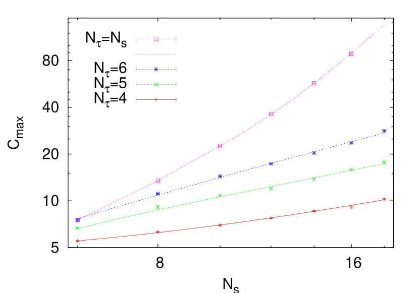
Figure 1: Maxima of the specific heat.

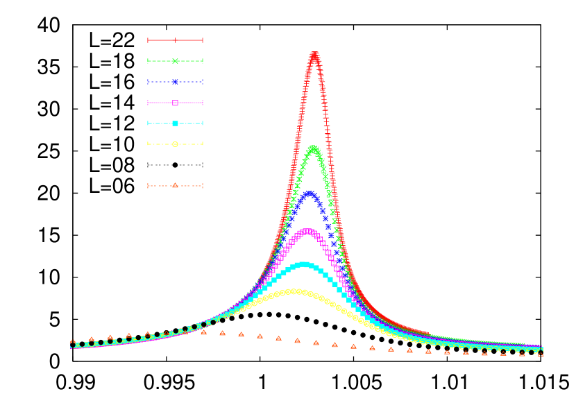
Figure 2: Polyakov loop susceptibilities for $N_{\tau}=4$.

The lattice size dependence of the maxima of the specific heat is shown in Fig. 1. For our symmetric lattices a fit to the first-order transition form

$$C_{\max}(N_{s})/(6N)=c_{0}+a_{1}/N+a_{2}/N^{2}$$ (8)

yields the estimate with $c_{0}\approx 0.00020$. Statistical error bars of our estimates can be found in [1]. Our $c_{0}$ value is 10% higher than the one reported in Rev. [9], where lattices up to size $18^{3}$ were used for this fit.

In contrast to symmetric lattices we find for $N_{\tau}=4$, 5 and 6 from Eqs. (2), (4), (5) and (7)

$$\frac{\alpha}{\nu}\approx 1\,,\qquad\frac{\gamma}{\nu}\approx 2\,,\qquad\frac{1-\beta}{\nu}\approx 1.5~{}~{}~{}~{}{\rm and}~{}~{}~{}~{}2-\eta\approx 2\ .$$ (9)

The hyperscaling relation $2-\alpha=d\nu$ with $d=3$ implies then $\alpha\approx\nu\approx 0.5$. For the Polyakov loop susceptibility and $N_{\tau}=4$ Fig. 2 shows our canonically reweighted data, implying $\gamma/\nu=2$ and, hence, $\gamma\approx 1$. For the reweighting the logarithmic coding from chapter 5.1.5 of [6] was used. From the derivative of $\langle|P|\rangle$ we get similarly $\beta\approx 0.25$, which is consistent with the scaling relation $\alpha+2\beta+\gamma=2$. While from the structure factor we find $2-\eta$ consistently with the scaling relation $\gamma/\nu=2-\eta$.

The exponents listed are the 3d Gaussian values. In view of statistical errors and expected systematic errors due to our limited lattice sizes, close-by values are as well possible. The problem with the Gaussian values is that the Gaussian renormalization group fixed point in 3d has two relevant operators [10]. So it is unstable and one does not understand why the effective spin system should care to converge into it [11]. Therefore, the interesting scenario of a new non-trivial fixed point with exponents accidentally close to 3d Gaussian arises. An illustration, which is consistent with the data, are the values $\nu=0.482$, $\alpha=0.554$, $\gamma=0.94$, $\beta=0.253$, $\eta=0.05$. Of course, we cannot entirely exclude that finite lattices mislead us and that really large systems turn either towards a first order transition or the 3d XY fixed point.

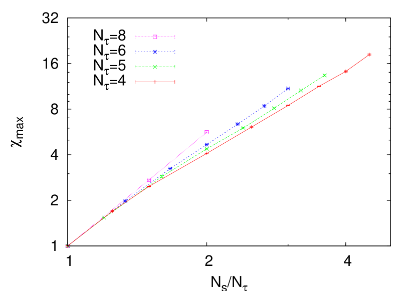
Figure 3: Rescaled maxima of Polyakov loops susceptibilities.

U(1) LGT in the $N_{t}\,N_{s}^{3},\,N_{s}>N_{\tau}$ geometry has previously only been studied by Vettorazzo and de Forcrand [12]. While their result for $N_{\tau}=4$ are consistent with a second order transition, they claim first order transitions for $N_{\tau}=6$ and 8. However, their $N_{\tau}=6$ and 8 data on very large lattices may simply exhibit the critical slowing down, which is typical for second order transitions [1]. For $N_{\tau}=4,$ 5 and 6 our data support, independently of $N_{\tau}$, the same critical exponent. We illustrate this here by rescaling the maxima of our Polyakov loop susceptibilities with a common factor, so that they become equal to 1 on symmetric lattices. On a log-log scale the results are then plotted in Fig. 3 against $N_{s}/N_{\tau}$. The behavior is certainly consistent with assuming a common critical exponent for all of them (parallel lines are expected for large $N_{s}/N_{\tau}$). The figure includes also some preliminary $N_{\tau}=8$ data, which so far blend in.

3 Summary and Conclusions

The litmus test for identifying a second order phase transitions is that one is able to calculate its critical exponents unambiguously. With MC calculations and FSS methods this finds its limitations through the lattice sizes, which fit into the computer and can be simulated in a reasonable time. Our lattice sizes are not small on the scale of typical numerical work on U(1) LGT, for instance the lattices used for the $c_{0}$ estimate of [9]. However, in view of the fact that our data do not support the generally expected scenarios, it would be desirable to extent the present analysis to lattices up to, say, size $32^{4}$. Using supercomputers this appears feasible. With mass spectrum methods [13], see [14] for recent work, one may investigate the scaling behavior of the model from a different angle. Finally, renormalization group theory could contribute to clarifying the issues raised by our data.

- [1] B.A. Berg and A. Bazavov, hep-lat/0605019.
- [2] B.A. Berg and T. Neuhaus, Phys. Lett. B 267, 249 (1991).
- [3] F. Wang and D.P. Landau, Phys. Rev. Lett 86, 2050 (2001).
- [4] A. Bazavov and B.A. Berg, Phys. Rev. D 71, 114506 (2005).
- [5] S.L. Adler, Phys. Rev. D 37, 458 (1981).
- [6] B.A. Berg, Markov Chain Monte Carlo Simulations and Their Statistical Analysis, World Scientific, Singapore, 2004.
- [7] A. Pelissetto and E. Vicari, Phys. Rep. 368, 549 (2002) [cond-mat/0012164].
- [8] H.E. Stanley, Introduction to Phase Transitions and Critical Phenomena, Clarendon Press, Oxford, 1971, pp. 98.
- [9] G. Arnold, B. Bunk, T. Lippert, and K. Schilling, Nucl. Phys. B (Proc. Suppl.) 119, 864 (2003) [hep-lat/0210010]; G. Arnold, T. Lippert, T. Neuhaus, and K. Schilling, Nucl. Phys. B (Proc. Suppl.) 94, 651 (2001) [hep-lat/0011058] and references given therein.
- [10] E.g., F.J. Wegner, in Phase Transitions and Critical Phenomena, C. Domb and M.S. Green editors (Academic Press, New York, 1976), p.59.
- [11] B. Svetitsky and L.G. Yaffe, Nucl. Phys. B 210, 423 (1982).
- [12] M. Vettorazzo and P. de Forcrand, Phys. Lett. B 604, 82 (2004) [hep-lat/0409135].
- [13] B.A. Berg and C. Panagiotakopoulos, Phys. Rev. Lett. 52, 94 (1984).
- [14] P. Majumdar, Y. Koma, and M. Koma, Nucl. Phys. B 677, 273 (2004) [hep-lat/0309003]; L. Tagliacozzo, Phys. Lett. B, to appear, [hep-lat/0603022].