The pion form factor from lattice QCD
with two dynamical flavours

Abstract

We compute the electromagnetic form factor of the pion using non-perturbatively $O(a)$ improved Wilson fermions. The calculations are done for a wide range of pion masses and lattice spacings. We check for finite size effects by repeating some of the measurements on smaller lattices. The large number of lattice parameters we use allows us to extrapolate to the physical point. For the square of the charge radius we find $\left<r^{2}\right>=0.441(19)~{}\text{fm}^{2}$, in good agreement with experiment.

1 Introduction

For some time now it has been possible to explore the structure of hadrons from first principles using lattice QCD. Since the pion is the lightest QCD bound state and plays a central role in chiral symmetry breaking and in low-energy dynamics, a thorough investigation of its internal structure in terms of quark and gluon degrees of freedom should be particularly interesting. We have started to explore the structure of the pion in a framework using generalised parton distributions, or more precisely their moments [1]. As a generalisation of parton distributions and form factors they contain both as limiting cases. In this work we restrict ourselves to results for the pion electromagnetic form factor $F_{\pi}$ from $N_{f}=2$ lattice QCD simulations, based on $O(a)$ improved Wilson fermions and Wilson glue. Initial studies on the pion form factor by Martinelli et al. and Draper et al. [2, 3] were followed by recent simulations in quenched [4, 5, 6, 7] and unquenched QCD [8, 9]. In this work, we improve upon previous calculations by extracting the pion form factor for a much larger number of $\beta$, $\kappa$ combinations, which allows us to study both the chiral and the continuum limit. Furthermore, two finite size runs make estimates of the volume effect possible.

2 The pion form factor in lattice QCD

The pion electromagnetic form factor $F_{\pi}$ describes how the vector current

$$V_{\mu}(x)=\textstyle{\frac{2}{3}}\,\overline{u}(x)\gamma_{\mu}u(x)-\textstyle{\frac{1}{3}}\,\overline{d}(x)\gamma_{\mu}d(x)$$ (1)

couples to the pion. Writing $p$ and $p^{\prime}$ for the incoming and outgoing momenta of the pion, it is defined by

$$\left<\pi^{+}(p^{\prime})\right|V_{\mu}(0)\left|\pi^{+}(p)\right>=(p^{\prime}_{\mu}+p^{\phantom{{}^{\prime}}}_{\mu})\,F_{\pi}(Q^{2})\,,$$ (2)

where the momentum transfer is $q_{\mu}=(p^{\prime}_{\mu}-p^{\phantom{{}^{\prime}}}_{\mu})$ and its invariant square is $q^{2}=-Q^{2}$.

For our lattice calculation we want to simplify the flavour structure of Eq. (1). Invoking isospin symmetry one finds

$$\left<\pi^{+}\right|\textstyle{\frac{2}{3}}\overline{u}\gamma_{\mu}u-\textstyle{\frac{1}{3}}\overline{d}\gamma_{\mu}d\left|\pi^{+}\right>=\\ \left<\pi^{+}\right|\overline{u}\gamma_{\mu}u\left|\pi^{+}\right>=-\left<\pi^{+}\right|\overline{d}\gamma_{\mu}d\left|\pi^{+}\right>\,.$$ (3)

It is hence sufficient to limit the calculation to a single quark flavour in the vector operator. We use the unimproved local vector current on the lattice; the corrections due to the improvement term [10] are quite small and will be discussed later. Since this current is not conserved, renormalisation has to be taken into account. Because in the forward limit ($Q^{2}=0$) the form factor is simply the electric charge of the pion, we can normalise our data appropriately. We can also use the known renormalisation constant $Z_{V}$ (taken for example from [11]) as a cross-check for our simulation.

To compute the matrix elements in Eq. (2) on the lattice, one has to evaluate pion three-point and two-point functions. We then apply a standard procedure to extract the pion form factor $F_{\pi}$, where one constructs an appropriate ratio for the observable [12, 13]. Let us start by looking at the three-point function. The general form is given by the correlation function

$$C_{\text{3pt}}(t,\vec{p}\,^{\prime},\vec{p}\,)=\left<{\eta_{\pi}^{\phantom{\dagger}}(t_{\text{sink}},\vec{p}\,^{\prime})\,\;\overline{u}(t)\gamma_{\mu}u(t)\,\;\eta_{\pi}^{\dagger}(t_{\text{source}},\vec{p}\,)}\right>$$ (4)

and depicted in Fig. 1. Here we denote the sink and source operators for a pion with given momentum and at given time-slice by $\eta_{\pi}(t_{\text{sink}},\vec{p}\,^{\prime})$ and $\eta_{\pi}^{\dagger}(t_{\text{source}},\vec{p}\,)$, respectively. Using the transfer matrix formalism and inserting complete sets of energy eigenstates, the three-point function is then of the form

$$C_{\text{3pt}}(t,\vec{p}\,^{\prime},\vec{p}\,)=\left<\pi(\vec{p}\,^{\prime})\right|\overline{u}(0)\gamma_{\mu}u(0)\left|\pi(\vec{p}\,)\right>\frac{\left<0\right|\eta_{\pi}(\vec{p}\,^{\prime})\left|\pi(\vec{p}\,^{\prime})\right>\left<\pi(\vec{p}\,)\right|\eta_{\pi}^{\dagger}(\vec{p}\,)\left|0\right>}{2E_{p^{\prime}}\,2E_{p}}\\ \times\left(\text{e}^{-E_{p^{\prime}}(t_{\text{sink}}-t)-E_{p}\,t}+(-1)^{n_{4}}\,\text{e}^{-E_{p^{\prime}}(t-t_{\text{sink}})-E_{p}\,(T-t)}\right)+\cdots\,,$$ (5)

where $T$ is the time extent of our lattice and

$$n_{4}=\left\{\begin{array}[]{l}1\text{~{}~{}for~{}}\mu=4\,,\\ 0\text{~{}~{}otherwise.}\end{array}\right.$$ (6)

Note that we have omitted excited states in Eq. (5) and already inserted our choice for the time-slice of the pion source, $t_{\text{source}}=0$. We choose the sink of the three-point function as $t_{\text{sink}}=T/2$, so that the correlation function is symmetric or antisymmetric with respect to this time,

$$C_{\text{3pt}}(t,\vec{p}\,^{\prime},\vec{p}\,)=(-1)^{n_{4}}\,C_{\text{3pt}}(T-t,\vec{p}\,^{\prime},\vec{p}\,).$$ (7)

We can then separate the correlation function into contributions from $t$ to the left and to the right of $t_{\text{sink}}$ (referred to as l.h.s. and r.h.s. in the following) and neglect either the second or first term in Eq. (5) since it is exponentially suppressed in the regions of $t$ from which we will extract the form factor.

Figure 1: A sketch of the three-point function with the pion source at time 0, pion sink at $t_{\text{sink}}$, and the operator acting at time $t$.

The two-point function has the form

$$C_{\text{2pt}}(t,\vec{p}\,)=\frac{\left<0\right|\eta_{\pi}(\vec{p}\,)\left|\pi(\vec{p}\,)\right>\left<\pi(\vec{p}\,)\right|\eta_{\pi}^{\dagger}(\vec{p}\,)\left|0\right>}{2E_{p}}\text{e}^{-E_{p}T/2}\,2\cosh[E_{p}(T/2-t)]+\cdots\,,$$ (8)

where again we omitted higher energy states. Comparing the two- and three-point functions (8) and (5), a ratio can be constructed that eliminates the overlap factors such as $\left<0\right|\eta_{\pi}(\vec{p}\,^{\prime})\left|\pi(\vec{p}\,^{\prime})\right>$ and partially cancels the exponential time behaviour appearing in Eq. (5). This technique also has the advantage that fluctuations of the correlation functions tend to cancel in the ratio and we thus obtain a better signal. With our choice $t_{\text{sink}}=T/2$, such a ratio is

$$R(t)=\frac{C_{\text{3pt}}(t,\vec{p}\,^{\prime},\vec{p}\,)}{C_{\text{2pt}}(t_{\text{sink}},\vec{p}\,^{\prime})}\;\left[\frac{C_{\text{2pt}}(t_{\text{sink}}-t,\vec{p}\,)\,C_{\text{2pt}}(t,\vec{p}\,^{\prime})\,C_{\text{2pt}}(t_{\text{sink}},\vec{p}\,^{\prime})}{C_{\text{2pt}}(t_{\text{sink}}-t,\vec{p}\,^{\prime})\,C_{\text{2pt}}(t,\vec{p}\,)\,C_{\text{2pt}}(t_{\text{sink}},\vec{p}\,)}\right]^{\!\frac{1}{2}}\,.$$ (9)

Similar ratios have already been used in earlier works on pion and nucleon structure. Here we take the somewhat more complicated ratio (9), which was used for the nucleon in [12], because we use momentum combinations with $|\vec{p}\,|\neq|\vec{p}\,^{\prime}|$. Contributions to this ratio from excited states with energy $E^{\prime}$ are suppressed as long as $t_{\text{sink}}-t\gg 1/(E^{\prime}-E)$ and $t\gg 1/(E^{\prime}-E)$ where $E$ is the pion energy. A potential problem is that, due to the exponential decay of the pion two-point function, the signal at $t=t_{\text{sink}}$ for non-vanishing momenta is poor. For finite statistics the two-point function can then take negative values, which prevents one from evaluating the square root. We try to overcome this difficulty by shifting the two-point functions $C_{\text{2pt}}(t,\vec{p}\,)$ that enter with $t=t_{\text{sink}}$. Using the identity

$$C_{\text{2pt}}(t_{\text{sink}},\vec{p})=\frac{C_{\text{2pt}}(t_{\text{sink}}-t_{\text{shift}},\vec{p})}{\cosh(E_{p}\,t_{\text{shift}})}$$ (10)

valid for $t_{\text{sink}}=T/2$, we shift by $t_{\text{shift}}=6$, which significantly reduces the number of negative two-point functions. Nevertheless there are still momentum transfers $Q^{2}$ for which the argument of the square root in the ratio (9) is negative. Those values are discarded when we evaluate the form factor.

For $Q^{2}\neq 0$ the ratio (9) does not exhibit a proper plateau that could immediately be used for fitting. This is due to our choice for $t_{\text{sink}}$, for which the time dependence of the pion two-point function cannot be approximated by a single exponential in the $t$ regions we use to extract the form factor, see Eq. (8). In fact, we now show that the ratio is approximately antisymmetric around the central point $t=t_{\text{sink}}/2=T/4$ of the l.h.s. (as well as around $t=3T/4$ on the r.h.s.). Defining $\delta\equiv t-t_{\text{sink}}/2$ and expanding the ratio and its exponentials in Eq. (9) around $\delta=0$ we find

$$R(t)=C(E_{p},E_{p^{\prime}},Q^{2})\left[1+2\delta\,c_{\delta}(E_{p},E_{p^{\prime}})+2\delta^{2}\,c_{\delta}^{2}(E_{p},E_{p^{\prime}})+\mathcal{O}(\delta^{3})\right]\,,$$ (11)

where

$$c_{\delta}(E_{p},E_{p^{\prime}}) = \frac{E_{p^{\prime}}}{1+\mathrm{e}^{E_{p}\,t_{\text{sink}}}}-\frac{E_{p}}{1+\mathrm{e}^{E_{p^{\prime}}\,t_{\text{sink}}}}\,,$$

$$C(E_{p},E_{p^{\prime}},Q^{2}) = \frac{(p^{\prime}_{\mu}+p^{\phantom{{}^{\prime}}}_{\mu})}{4\sqrt{E_{p^{\prime}}E_{p}}}\,F_{\pi}(Q^{2})\,.$$ (12)

When averaging $R(t)$ in a symmetric interval around $t=T/4$, the antisymmetric piece proportional to $c_{\delta}$ in (11) drops out. However, such an averaged signal also includes unwanted symmetric contributions. Fortunately, for our pion masses and lattice momenta already the leading symmetric term is negligible, because with the lattice spacing $a$ we have $c_{\delta}^{2}\sim 10^{-4}a^{-2}$ and $\delta^{2}\leq 4a^{2}$ in our fits. We hence obtain a good signal for the averaged ratio. The same is true for the r.h.s. ratio and its central point $t=3T/4$. A typical ratio at non-zero momentum transfer is shown in Fig. 2 for one of our data sets, along with the familiar plateau for zero momentum transfer. Note that the ratio (9) does not exhibit a plateau for arbitrary momenta. To visualise the absence of possible contributions from excited states one has to consider the ratio for $|\vec{p}\,|=|\vec{p}\,^{\prime}|$. In this case the time dependence of the three-point function (5) should vanish. We have checked that this is indeed the case in the region we average over, within the expected increase of noise for higher momenta or lower pion masses.

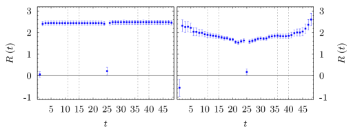
Figure 2: Examples of the ratio $R(t)$ in Eq. (9) on the $24^{3}\times 48$ lattice at $\beta=5.25$, $\kappa=0.13575$, multiplied with an appropriate sign factor $(-1)^{n_{4}}$ for $t>t_{\text{sink}}$. The left plot shows a proper plateau in the forward case $Q^{2}=0$ and the right plot shows the ratio for $Q^{2}=0.31{\,\text{Ge}\kern-0.66666pt\text{V\/}}^{2}$ where no plateau is expected (see text). The dashed lines indicate the regions we average over.

From Eqs. (11) and (2) we see that the lattice ratio (9) can be used to extract the form factor $F_{\pi}(Q^{2})$. Using then several combinations of momenta $p$ and $p^{\prime}$ that all give the same $Q^{2}$ provides an over-constrained set of equations, from which we determine $F_{\pi}(Q^{2})$ by $\chi^{2}$ minimisation. We increase the quality of our signal by averaging the ratio over the contributions on the l.h.s. and r.h.s. This requires the additional sign factor $(-1)^{n_{4}}$ between the two sides, as can be seen in Eq. (7). The energies $E_{p}$ and $E_{p^{\prime}}$ appearing in (10) and (2) are calculated using the lattice pion masses and the continuum dispersion relation. We also performed a test of the dispersion relation for some of our lattices. It was increasingly difficult to extract a signal for higher momenta, especially for the lowest pion masses. However, we found that the continuum dispersion relation can be used to describe the data and that a lattice dispersion relation is not favoured.

3 Simulation details

We perform our simulations with two flavours of non-perturbatively clover-improved dynamical Wilson fermions and Wilson glue. Using these actions, the QCDSF and UKQCD collaborations have generated gauge field configurations with the parameters given in Table 1, where we have used the Sommer parameter with $r_{0}=0.467$ fm (see [14] and [15]) to set the physical scale. This large set of lattices enables us to extrapolate to the chiral and the continuum limit. For two sets of parameters ($\beta=5.29$, $\kappa=0.1355,0.1359$) we also have a choice of lattice volumes ($12^{3}\times 32$, $16^{3}\times 32$ and $24^{3}\times 48$) in order to study finite volume effects.

Table 1: Overview of our lattice parameters. For physical units the Sommer parameter with $r_{0}=0.467$ fm has been used. The error on $m_{\pi}$ is purely statistical.

$\beta$	#	$\kappa$	$N^{3}\times T$	$m_{\pi}$ [GeV]	$a$ [fm]	$L$ [fm]	$N_{\text{traj}}$
5.20	1	0.13420	$16^{3}\times 32$	1.007(2)	0.115	1.8	$\mathcal{O}(5000)$
	2	0.13500	$16^{3}\times 32$	0.833(3)	0.098	1.6	$\mathcal{O}(8000)$
	3	0.13550	$16^{3}\times 32$	0.619(3)	0.093	1.5	$\mathcal{O}(8000)$
5.25	4	0.13460	$16^{3}\times 32$	0.987(2)	0.099	1.6	$\mathcal{O}(5800)$
	5	0.13520	$16^{3}\times 32$	0.829(3)	0.091	1.5	$\mathcal{O}(8000)$
	6	0.13575	$24^{3}\times 48$	0.597(1)	0.084	2.0	$\mathcal{O}(5900)$
5.26	7	0.13450	$16^{3}\times 32$	1.011(3)	0.099	1.6	$\mathcal{O}(4000)$
5.29	8	0.13400	$16^{3}\times 32$	1.173(2)	0.097	1.6	$\mathcal{O}(4000)$
	9	0.13500	$16^{3}\times 32$	0.929(2)	0.089	1.4	$\mathcal{O}(5600)$
	10	0.13550	$24^{3}\times 48$	0.769(2)	0.084	2.0	$\mathcal{O}(2000)$
	11	0.13590	$24^{3}\times 48$	0.591(2)	0.080	1.9	$\mathcal{O}(5900)$
	12	0.13620	$24^{3}\times 48$	0.400(3)	0.077	1.9	$\mathcal{O}(5600)$
5.40	13	0.13500	$24^{3}\times 48$	1.037(1)	0.077	1.8	$\mathcal{O}(3700)$
	14	0.13560	$24^{3}\times 48$	0.842(2)	0.073	1.8	$\mathcal{O}(3500)$
	15	0.13610	$24^{3}\times 48$	0.626(2)	0.070	1.7	$\mathcal{O}(3900)$

Starting with the lattice version of the three-point function, Eq. (4), we follow [16] and find that it is sufficient to calculate

$$\sum_{\vec{y}}\,\sum_{\vec{z}}\mathrm{e}^{-\mathrm{i}\vec{p}\,^{\prime}\cdot\vec{y}}\,\mathrm{e}^{\mathrm{i}\vec{q}\cdot\vec{z}}\left<\mathrm{Tr}\;\Gamma G(y,z)\gamma_{\mu}G(z,x)\Gamma^{\dagger}G(x,y)\right>_{g}$$ (13)

with $x_{4}=0$, $y_{4}=T/2$, $z_{4}=t$. Here $G(y,z)$ is the fermion propagator, the average is taken over the gauge fields, and the trace is over the suppressed Dirac and colour indices. The matrix $\Gamma$ represents the Dirac structure of the pion interpolating field $\eta_{\pi}$, while the Fourier transformations ensure that we have fixed momenta at the operator insertion and the sink.

We use two different pion interpolating fields to create the pions on the lattice, namely a pseudo-scalar and the fourth component of the axial-vector current, which both have the correct quantum numbers. For a given momentum $\vec{p}$ they read

$$\eta_{\pi}(t,\vec{p}\,)=\sum_{\vec{x}}\mathrm{e}^{-\mathrm{i}\vec{p}\cdot\vec{x}}\;\,\overline{d}(x)\,\Gamma\,u(x)\,,\qquad\Gamma=\gamma_{5}\text{ or }\gamma_{4}\gamma_{5}$$ (14)

with $x_{4}=t$. We apply Jacobi smearing [17] at the source as well as the sink to increase the overlap of the lattice interpolating fields with the physical pion states.

The three-point function (13) is then evaluated by applying the sequential source technique as indicated in Fig. 1. This makes it efficient to use a large number of momentum transfers, as required for calculating form factors. A large set of momenta is necessary to assess the $Q^{2}$ dependence, and having several combinations of $\vec{p}\,^{\prime}$ and $\vec{q}$ belonging to the same $Q^{2}$ makes the fits more reliable. We use three final momenta $\vec{p}\,^{\prime}$ and 17 momentum transfers $\vec{q}$, giving a total of 51 combinations for an over-constrained fit for $F_{\pi}$ at 17 different values of $Q^{2}$. In units of $2\pi/L$ the momenta are given by

$$\vec{p}\,^{\prime}\!\!\! = (0,0,0),(0,1,0),(1,0,0),$$

$$\vec{q} = (0,0,0),(-1,0,0),(-1,-1,0),(-1,-1,-1),$$

$$(-2,0,0),(-2,-1,-1),(-2,-2,-1),\cdots$$

where $\cdots$ stands for all possible permutations w.r.t. the components. The errors we quote for our results are statistical errors obtained by the jackknife method.

4 Experimental data for the pion form factor

Let us now take a brief look at the experimental measurements of $F_{\pi}(Q^{2})$ to which we compare our lattice results. Very accurate data up to $Q^{2}=0.253{\,\text{Ge}\kern-0.66666pt\text{V\/}}^{2}$ have been obtained in [18] from elastic scattering of a pion beam on the shell electrons of the target material. At higher $Q^{2}$ the pion form factor has been extracted from $ep\to en\pi^{+}$, which is considerably more involved (see [19] for a recent discussion). We only use here data from [20, 21, 22], where the cross sections for longitudinal and transverse photons have been experimentally separated by the Rosenbluth method. Together these data span a range from $Q^{2}=0.35{\,\text{Ge}\kern-0.66666pt\text{V\/}}^{2}$ to $2.45{\,\text{Ge}\kern-0.66666pt\text{V\/}}^{2}$.

We find the experimental data on $F_{\pi}$ well described by a monopole form

$$F_{\pi}(Q^{2})=\frac{1}{1+Q^{2}/M^{2}},$$ (16)

with a fit of the combined data from [18, 20, 21, 22] giving $M=0.714(4){\,\text{Ge}\kern-0.66666pt\text{V\/}}$ at $\chi^{2}/\text{d.o.f.}=1.27$. This is remarkably close to the result $M=0.719(5){\,\text{Ge}\kern-0.66666pt\text{V\/}}$ at $\chi^{2}/\text{d.o.f.}=1.13$ obtained when fitting only the data of [18] with its much smaller range in $Q^{2}$, which illustrates the stability of a monopole form up to $2.45{\,\text{Ge}\kern-0.66666pt\text{V\/}}^{2}$.

The low-$Q^{2}$ behaviour of $F_{\pi}$ is characterised by the squared charge radius

$$\langle r^{2}\rangle=-6\,\left.\frac{\mathrm{d}F_{\pi}(Q^{2})}{\mathrm{d}Q^{2}}\right|_{Q^{2}=0}.$$ (17)

For a monopole form (16) one has

$$\langle r^{2}\rangle=6/M^{2}.$$ (18)

In Table 2 we list the values obtained from a number of fits to $F_{\pi}$. The PDG average [24] uses results from form factor data at both spacelike and timelike virtualities. The three fits to the Amendolia data [18] illustrate that different fitting procedures can give results with a variation much bigger than the quoted statistical and systematic errors. Fit 1 (whose result is the one retained in the PDG average) is based on a representation of $F_{\pi}$ as a dispersion integral. Fit 2 was also given in [18] and assumed a monopole form (16) with a normalisation factor allowed to deviate from 1 by $\pm 0.9\%$, which corresponds to the overall normalisation uncertainty of the measurement. Fit 3 assumes a monopole form with normalisation fixed to 1, as does the fit to the combined data of [18, 20, 21, 22].

Table 2: Values of the squared pion charge radius obtained from different data sets for $F_{\pi}(Q^{2})$ and with different fitting assumptions. Details of the fits are given in the text.

data	$\langle r^{2}\rangle$ [fm2]
global average, PDG 2004 [24]	$0.452(11)$
Amendolia [18], fit 1	$0.439(8)$
Amendolia [18], fit 2	$0.431(10)$
Amendolia [18], fit 3	$0.451(6)$
combined data [18, 20, 21, 22]	$0.458(5)$

5 Results

5.1 Fits to lattice data and extrapolation in $m_{\pi}$

We start the discussion of our results by explaining our fitting procedure, including combined fits to all data sets. In the next subsection we will argue that lattice artifacts are small. To obtain the physical form factor we have to renormalise our lattice result, $F^{\text{ren}}_{\pi}=Z_{V}F^{\text{bare}}_{\pi}$. As mentioned in Section 2, we can do this by using the electric charge of the pion as input, i.e.

$$F^{\text{lat,ren}}_{\pi}(Q^{2})=\frac{F^{\text{lat,bare}}_{\pi}(Q^{2})}{F^{\text{lat,bare}}_{\pi}(0)}\,,$$ (19)

so that $F^{\text{lat,ren}}_{\pi}(0)=F^{\text{phys}}_{\pi}(0)=1$. We then use a monopole ansatz to fit the actual data for the form factor

$$F^{\text{lat}}_{\pi}(Q^{2})=\frac{1}{1+Q^{2}/M_{\text{lat}}^{2}}\,,$$ (20)

where we have $M_{\text{lat}}$ as a fit parameter for each of our lattices at its lattice pion mass $m_{\pi,\text{lat}}$. The quality of this fitting ansatz will be discussed below.

Using this fitting function, we compare the results obtained with the two pion interpolating fields (14) and observe several differences. In general, the matrix elements for pions using $\Gamma=\gamma_{4}\gamma_{5}$ display a slightly cleaner signal with more data points in $Q^{2}$, i.e. less contamination due to negative two-point functions. Fitting the monopole form (20) to the form factor for both pion interpolators we find that the $\chi^{2}/\text{d.o.f.}$ differs on average by about a factor of 2, ranging from 0.18 – 1.72 (0.23 – 3.49) for the interpolator with $\gamma_{4}\gamma_{5}$ ($\gamma_{5}$). The fitted monopole masses for the $\Gamma=\gamma_{5}$ pions lie consistently above the ones for $\Gamma=\gamma_{4}\gamma_{5}$ but agree within errors for most lattices. In an exploratory extraction of the pion energies from the two-point functions with non-vanishing momentum on a sub-set of our lattices, we also found that the pseudo-scalars with $\Gamma=\gamma_{5}$ had a worse signal at higher momenta. A similar observation was made in [8] and may explain the difference in quality of the form factors extracted from the two pion currents. Because of the better signal, we will mainly discuss results for the pions created with $\Gamma=\gamma_{4}\gamma_{5}$ in the remainder of this work.

To obtain the pion form factor at the physical pion mass we extrapolate the values for $M_{\text{lat}}$, given in Table 3, to the physical point. We tried different extrapolations in the square of the pion mass, see Table 4, including also a fit inspired by chiral perturbation theory and used in [9]. For the latter we chose the fit range of $m^{2}_{\pi,\text{lat}}<0.8{\,\text{Ge}\kern-0.66666pt\text{V\/}}^{2}$. Varying this fit range within reasonable bounds did not have a significant effect on the extrapolated value of $M_{\text{phys}}$. We find the best $\chi^{2}$ value for fit 2, where $M_{\text{lat}}^{2}$ depends linearly on $m_{\pi}^{2}$. The extrapolations in the remainder of this paper are based on this ansatz. We will however include an estimated systematic error of $\Delta M_{\text{ext}}=35{\,\text{Me}\kern-0.66666pt\text{V\/}}$ from the difference of fits 1 and 2 in our final result (this is bigger than the difference between fits 1 and 4, whereas fit 3 gives a significantly worse description of the data). Figure 3 shows the extrapolation to the physical pion mass based on fits 2 and 4. We remark that our lattice with the lowest pion mass, $m_{\pi}=400{\,\text{Me}\kern-0.66666pt\text{V\/}}$, is completely consistent and increases our confidence in the fit and fit ansatz. However, due to the larger statistical errors it has little weight in this result: when leaving it out of the fit $M_{\text{phys}}$ changes only by $1{\,\text{Me}\kern-0.66666pt\text{V\/}}$. The corresponding run and several others at small pion masses are still in progress. It is obvious that one needs higher statistics for this point to be significant.

Table 3: Monopole masses $M_{\text{lat}}$ obtained from fits to (20) for each of our lattices. The last column gives an estimate for the shift $\Delta M_{\text{lat}}=M(m_{\pi}^{2},\infty)-M(m_{\pi}^{2},L)$ of the monopole mass due to finite volume effects. It is obtained from the empirical fit (26) discussed in Section 5.2.

#	$m_{\pi}$ [GeV]	$L$ [fm]	$m_{\pi}L$	$M_{\text{lat}}~{}[{\text{Ge}\kern-0.66666pt\text{V\/}}]$	$\Delta M_{\text{lat}}~{}[{\text{Me}\kern-0.66666pt\text{V\/}}]$
1	1.007(2)	1.8	9.4	1.104(22)	0	.3
2	0.833(3)	1.6	6.6	0.997(21)	4	.3
3	0.619(3)	1.5	4.7	0.880(24)	35	.2
4	0.987(2)	1.6	7.9	1.089(20)	1	.1
5	0.829(3)	1.5	6.1	0.975(17)	7	.2
6	0.597(1)	2.0	6.1	0.870(22)	8	.0
7	1.011(3)	1.6	8.1	1.066(25)	0	.9
8	1.173(2)	1.6	9.2	1.157(20)	0	.3
9	0.929(2)	1.4	6.7	1.051(15)	3	.7
10	0.769(2)	2.0	7.8	0.971(14)	1	.3
11	0.591(2)	1.9	5.7	0.854(15)	12	.6
12	0.400(3)	1.9	3.8	0.783(36)		–
13	1.037(1)	1.8	9.7	1.099(13)	0	.2
14	0.842(2)	1.8	7.5	0.981(14)	1	.8
15	0.626(2)	1.7	5.3	0.847(17)	18	.2

Table 4: Different forms used to extrapolate the monopole mass to the physical value of $m_{\pi}$. In fit 4 we have $L=1/(4\pi f)^{2}\log(m^{2}_{\pi,\text{lat}}/\mu^{2})$, where $\mu=1{\,\text{Ge}\kern-0.66666pt\text{V\/}}$ and $f_{\pi}\approx 92{\,\text{Me}\kern-0.66666pt\text{V\/}}$ is the pion decay constant.

#	extrapolation ansatz	$\chi^{2}$/d.o.f.	$c_{1}$		$M_{\text{phys}}$ [GeV]
1	$M_{\text{lat}}^{\phantom{2}}=c_{0}+c_{1}m^{2}_{\pi,\text{lat}}$	1.31	0.322(15)	${\,\text{Ge}\kern-0.66666pt\text{V\/}}^{-1}$	0.	761(13)
2	$M_{\text{lat}}^{2}=c_{0}+c_{1}m^{2}_{\pi,\text{lat}}$	0.93	0.647(30)		0.	726(16)
3	$1/M_{\text{lat}}^{2}=c_{0}+c_{1}m^{2}_{\pi,\text{lat}}\rule[-4.73611pt]{0.0pt}{10.76385pt}$	3.25	$-0.575(31)$	${\,\text{Ge}\kern-0.66666pt\text{V\/}}^{-4}$	0.	833(9)
4	$6/M_{\text{lat}}^{2}=c_{0}+c_{1}m^{2}_{\pi,\text{lat}}-L$	1.11	$-4.33(62)$	${\,\text{Ge}\kern-0.66666pt\text{V\/}}^{-4}$	0.	715(4)

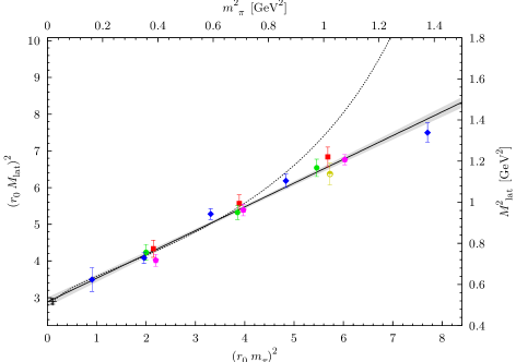
Figure 3: Extrapolations of the squared monopole mass against the squared pion mass. The solid line with error band is linear extrapolation as obtained from fit 2 while the dotted line shows the central curve for fit 4 (whose fit range is limited to $m^{2}_{\pi}<0.8{\,\text{Ge}\kern-0.66666pt\text{V\/}}^{2}$). The cross marks the monopole mass corresponding to the PDG value [24] of the pion charge radius, see Eq. (18) and Table 2. The different symbols refer to our $\beta$-values: squares (5.20), circles (5.25), half-full circle (5.26), diamonds (5.29), and hexagons (5.40).

We include the $m_{\pi}$ dependence of the monopole mass of fit 2 in a combined fit to all our lattice data available. This fit has the same monopole form as in (20) with one additional parameter to incorporate the $m_{\pi}$ behaviour,

$$\begin{split}F_{\pi}(Q^{2},m_{\pi}^{2})&=\frac{1}{1+Q^{2}/M^{2}(m_{\pi}^{2})}\,,\\[3.99994pt] M^{2}(m_{\pi}^{2})&=c_{0}+c_{1}m^{2}_{\pi}\,.\end{split}$$ (21)

The two fit parameters, $c_{0}$ and $c_{1}$, describe the relation between the monopole mass and the pion mass, and we immediately obtain the form factor $F^{\text{phys}}_{\pi}(Q^{2})=F^{\phantom{h}}_{\pi}(Q^{2},m_{\pi,\text{phys}}^{2})$ in the physical limit. The fitted parameters are $c_{0}=0.517(23){\,\text{Ge}\kern-0.66666pt\text{V\/}}^{2}$ and $c_{1}=0.647(30)$ with $\chi^{2}/\text{d.o.f.}=0.64$. This gives $M_{\text{phys}}=M(m^{2}_{\pi,\text{phys}})=0.727(16){\,\text{Ge}\kern-0.66666pt\text{V\/}}$, in good agreement with the experimental result.

Figure 4 shows experimental data along with the combined fit with its extrapolated curve. For this plot, our data at the lattice pion masses is shifted to the physical pion mass and plotted on-top of the extrapolation. We do this by subtracting from the individual lattice points, $F^{\text{lat}}_{\pi}(Q^{2})$, a value $\bigr{(}F_{\pi}(Q^{2},m_{\pi,\text{lat}}^{2})-F_{\pi}(Q^{2},m_{\pi,\text{phys}}^{2})\bigr{)}$ calculated with the fit parameters of Eq. (21) at the respective pion masses. The errors are left unchanged. We find good agreement between our simulation and the experimental results. This is emphasised by the insert in Fig. 4, which shows the region $Q^{2}<1{\,\text{Ge}\kern-0.66666pt\text{V\/}}^{2}$, where most of the experimental points lie. The same fit for the pions with $\Gamma=\gamma_{5}$ gives $M_{\text{phys}}=0.773(17){\,\text{Ge}\kern-0.66666pt\text{V\/}}$, with a bigger $\chi^{2}/\text{d.o.f.}$ of 1.01.

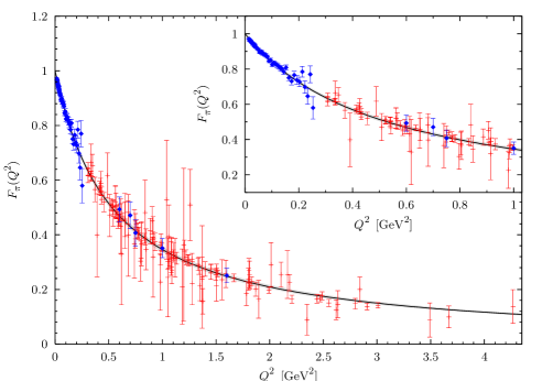
Figure 4: Combined fit to (21) of our data for all lattices. We plot experimental data (diamonds) [18, 21, 23] and lattice results extrapolated to the physical pion mass as explained in the text. To avoid having a cluttered plot we do not show lattice results with errors bigger than 80%, which are nevertheless included in the fit. The insert shows the good agreement to the experimental data for a momentum transfer of up to 1 GeV². Also included is an error band for the fit.

We now investigate the validity of the monopole ansatz for our data. Instead of constraining the fitting function to a monopole form, one can also take a general power law, i.e. use a function

$$\begin{split}F_{\pi}(Q^{2},m_{\pi}^{2})&=\left(1+\frac{Q^{2}}{p\mskip 1.5muM^{2}(m_{\pi}^{2})}\right)^{-p}\,,\\[3.99994pt] M^{2}(m_{\pi}^{2})&=c_{0}+c_{1}m^{2}_{\pi}\,,\end{split}$$ (22)

with an additional parameter, $p$. Note that the relation (18) is still valid, independent of $p$. A combined fit to all our data sets results in $p=1.173(58)$, now with a mass $M_{\text{phys}}=0.757(18){\,\text{Ge}\kern-0.66666pt\text{V\/}}$ and a $\chi^{2}/\text{d.o.f.}=0.58$, indicating that the monopole form is a good description. Taking the difference between this number and the result of the fit to (21), we assign a systematic error of $\Delta M_{\text{fit}}=30{\,\text{Me}\kern-0.66666pt\text{V\/}}$ to $M_{\text{phys}}$ due to the ansatz for the fitting function. Another alternative is to calculate an effective monopole mass for every momentum $Q^{2}$ separately by solving Eq. (20) for $M_{\text{lat}}$:

$$M_{\text{eff}}(Q^{2})=Q\left[\frac{1}{F^{\text{lat}}_{\pi}(Q^{2})}-1\,\right]^{-1/2}.$$ (23)

We show such effective masses for some of our lattices in Fig. 5, where one can see that the effective monopole masses stay constant within errors over a large range of $Q^{2}$ and agree with the monopole masses given in Table 3. This again indicates that the monopole is a good description for our data. The validity of the fit over the whole $Q^{2}$ range is further tested by combined fits to Eq. (21) in a limited fitting range $Q^{2}\leq Q^{2}_{\text{max}}$ or $Q^{2}_{\text{min}}\leq Q^{2}$. This is shown in Fig. 6, where we successively limit the fit to smaller (larger) momenta. Note that the increasing errors to the left or the right are due to the decrease in the number of fitted data points. Within these errors, the change in the monopole mass is consistent with statistical fluctuations. From Figs. 5 and 6 we can conclude that the monopole ansatz works well in the entire region for which we have lattice data, from $Q^{2}=0$ to about $4~{}{\text{Ge}\kern-0.66666pt\text{V\/}}^{2}$.

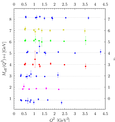
Figure 5: Effective monopole masses $M_{\text{eff}}(Q^{2})$ defined in (23), together with the corresponding monopole masses from Table 3 (dotted lines) for a sample of our lattices from small to large pion masses (lattices number 8, 7, 4, 9, 2, 10, 15, and 11 from top to bottom). For better visibility we omitted 2 points with very large errors in the plot, but included them in the fit.

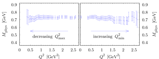
Figure 6: Combined fits to (21) with reduced fitting ranges in $Q^{2}$. For the left plot $Q^{2}_{\text{max}}$ is decreased, while $Q^{2}_{\text{min}}$ is increased for the right plot. We use bins of $50{\,\text{Me}\kern-0.66666pt\text{V\/}}^{2}$ and show only points where the number of data points in the fit of $F_{\pi}$ changed.

The results discussed so far have used the lattice data normalised as in (19). Using

$$Z_{V}F^{\text{lat,bare}}_{\pi}(0)=F_{\pi}^{\text{lat,ren}}(0)=1,$$ (24)

we can determine $Z_{V}$ from our (unrenormalised) data at zero momentum transfer. We find reasonable agreement with the values of $Z_{V}$ given in [11], albeit with errors that are larger by at least an order of magnitude. The bigger errors are likely due to our choice of $t_{\text{sink}}$, which results in noisier two-point functions.

5.2 Finite volume and discretisation effects

Let us now turn to the discussion of lattice artifacts. Apart from the extrapolation to the physical pion mass there are two more limits to be taken: the infinite volume limit and the continuum limit. The large number of lattices available allows us to investigate both. In order to study the volume dependence of our results, we make use of two sets of configurations that have the same parameters $\beta$, $\kappa$ for the lattice action but different volumes (see Table 5).

Table 5: Overview of our finite size runs. Note that we use the pion mass and lattice spacing of the largest lattice also for the smaller ones. They are given in Table 1 and not repeated here.

$\beta$	$\kappa$	#	$N^{3}\times T$	$L$ [fm]	$m_{\pi}L$	$M_{\text{lat}}[{\text{Ge}\kern-0.66666pt\text{V\/}}]$	$\Delta M_{\text{lat}}[{\text{Me}\kern-0.66666pt\text{V\/}}]$
5.29	0.13550	10	$24^{3}\times 48$	2.0	7.8	0.971(14)	1	.4
		10 a	$16^{3}\times 32$	1.3	5.2	0.928(16)	19	.7
		10 b	$12^{3}\times 32$	1.0	3.9	0.841(48)	75	.0
5.29	0.13590	11	$24^{3}\times 48$	1.9	5.7	0.854(15)	12	.6
		11 a	$16^{3}\times 32$	1.3	3.8	0.786(18)	90	.3
		11 b	$12^{3}\times 32$	1.0	2.9	0.513(31)	263	.1

In Fig. 7a we show the monopole masses fitted according to Eq. (20) as a function of the lattice size $L$. We use the pion mass $m_{\pi}$ and lattice spacing $a$ determined for the lattice with the largest volume also for the smaller ones. Figure 7b gives an overview of our lattices in the $m_{\pi}$–$L$ plane.

To obtain some understanding of the volume dependence one may have recourse to chiral perturbation theory. The volume dependence of the pion charge radius has been investigated to one-loop order in various approaches of chiral perturbation theory [25, 26, 27]. In the continuum limit, the result of the lattice regularised calculation in [27] amounts to a finite size correction of

$$\left<r^{2}\right>_{L}-\left<r^{2}\right>_{\infty}=\frac{3}{8\pi^{2}f^{2}_{\pi}}\sum_{\vec{n}\neq\vec{0}}K_{0}(Lm_{\pi}|\vec{n}|)\,,$$ (25)

where the sum runs over all three-vectors $\vec{n}\neq\vec{0}$ with integer components and $f_{\pi}\approx 92{\,\text{Me}\kern-0.66666pt\text{V\/}}$ is the pion decay constant. Note that the finite size correction of the charge radius is not proportional to $m^{2}_{\pi}$, unlike for other quantities such as the pion decay constant or the nucleon axial coupling. The leading contribution in Eq. (25) for large values of $m_{\pi}L$ is proportional to $K_{0}(m_{\pi}L)\sim\sqrt{\pi/(2m_{\pi}L)}\,\mathrm{e}^{-m_{\pi}L}$. Unfortunately we cannot expect chiral perturbation theory to be applicable at the pion masses and lattice volumes used in our simulations. This includes the result (25), which we take however as a guide for the functional form of the volume dependence. We thus change the monopole mass in (21) to

$$M^{2}(m_{\pi}^{2},L)=c_{0}+c_{1}m^{2}_{\pi}+c_{2}\mskip 1.5mu\mathrm{e}^{-m_{\pi}L}\,.$$ (26)

We then perform a combined fit to the data of all lattices in Table 1 except for number $12$ (see below), including in addition the $16^{3}\times 32$ lattices of the finite volume runs (numbers 10 a and 11 a). The result is represented by the solid lines in Fig. 7a. The fitted parameters are $c_{0}=0.553(29){\,\text{Ge}\kern-0.66666pt\text{V\/}}^{2}$, $c_{1}=0.612(35)$ and $c_{2}=-6.97(1.71){\,\text{Ge}\kern-0.66666pt\text{V\/}}^{2}$ at $\chi^{2}/\text{d.o.f.}=0.62$ which gives $M_{\text{phys}}=0.751(19){\,\text{Ge}\kern-0.66666pt\text{V\/}}$ for the infinite volume limit of the monopole mass at the physical point. Compared with the value $0.727(16){\,\text{Ge}\kern-0.66666pt\text{V\/}}$ obtained in the fit (21) without volume dependence, this represents a small overall finite-size effect. The fitted parameters do not change significantly if we only fit the $16^{3}\times 32$ and $24^{3}\times 48$ data sets of the finite volume runs, i.e. the data corresponding to the four rightmost points in Fig. 7a (lattices number 10, 10 a, 11, and 11 a). We have not included the $12^{3}\times 32$ lattices in the fit (26) since we cannot expect our simple ansatz to hold down to lattice sizes of 1 fm. Qualitatively, our fit is not too bad even in this region, as shown by the dotted lines in Fig. 7a.

With the fitted parameters we can estimate the finite volume shift for each of our lattices as given in Table 3. Except for a few lattices we find very small effects. We do not expect that with the simple form (26) fitted to our finite volume data at $m_{\pi}=591{\,\text{Me}\kern-0.66666pt\text{V\/}}$ and $m_{\pi}=769{\,\text{Me}\kern-0.66666pt\text{V\/}}$ (the dotted lines in Fig. 7b) we can estimate volume effects for pion masses as low as $400{\,\text{Me}\kern-0.66666pt\text{V\/}}$. We therefore have excluded lattice number $12$ from our finite volume investigation.

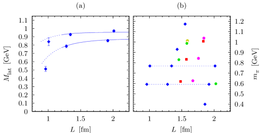
Figure 7: (a) Monopole mass vs. lattice size in our finite volume data sets with $\beta=5.29$ and $\kappa=0.1355$ (upper points) or $\kappa=0.1359$ (lower points). The curves correspond to a fit to (26) as discussed in the text. (b) Overview of pion masses and lattice sizes for our complete data set. The dotted lines mark our finite size runs.

Before discussing the scaling behaviour, let us briefly discuss the possibility of $\mathcal{O}(a)$ improving the local vector current. The improved current has the form

$$\begin{split}V^{\text{imp}}_{\mu}(x)&=\overline{u}(x)\gamma_{\mu}u(x)+c_{V}\mskip 1.5mua\partial_{\nu}T_{\mu\nu}(x)\,,\\[1.99997pt] T_{\mu\nu}(x)&=\mathrm{i}\,\overline{u}(x)\sigma_{\mu\nu}u(x)\,.\end{split}$$ (27)

The improvement coefficient $c_{V}$ is only known from lattice perturbation theory [10] because the only non-perturbative calculations to date are for quenched fermions (see e.g. [28]). However, even with tadpole improvement the perturbative value for our coarsest lattice is $c_{V}\approx-0.027$. This is so small that we expect no sizable effect on our results. To see this, we plot in Fig. 8 the ratio

$$r_{\text{imp}}(Q^{2})=\frac{\left<\pi(p^{\prime})\right|{a\partial_{\nu}T_{\mu\nu}}\left|\pi(p)\right>}{\left<\pi(p^{\prime})\right|{\overline{u}\gamma_{\mu}u}\left|\pi(p)\right>}$$ (28)

of the pion matrix elements for the two operators on the r.h.s. of Eq. (27). The dependence on the index $\mu$ cancels in this ratio. Note that here we use unrenormalised lattice data and that we still have to multiply with $c_{V}$ in order to obtain the effect of the improvement term in the current. This example plot is for our coarsest lattice ($\beta=5.20$ and $\kappa=0.1342$), where the improvement term should have the largest impact. To gain a feeling for the possible size of the effect, we used a fixed value of $c_{V}=-0.3$ to compute the effect on a sub-set of our lattices (lattices number 2, 6, 11, 15). Although this improvement coefficient is more than ten times larger than the tadpole improved value for our coarsest lattice, the shift of the monopole mass was moderate with 6 to 10%. Given the size of our statistical errors on $F_{\pi}$ and the fact that a reliable value for $c_{V}$ is not known for our lattices, we decided to neglect operator improvement and use the local vector current.

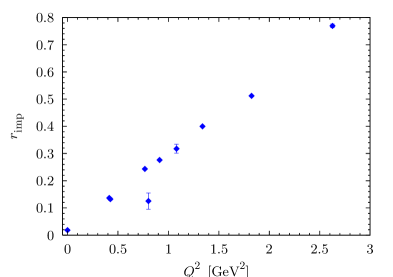
Figure 8: The ratio $r_{\text{imp}}(Q^{2})$ defined in Eq. (28), evaluated for our coarsest lattice ($\beta=5.20$, $\kappa=0.1342$). To obtain the effect of $\mathcal{O}(a)$ improving the current, this ratio needs to be multiplied with $c_{V}$.

We now investigate the scaling behaviour by extrapolating our values for the monopole mass to the physical pion mass separately for each $\beta$ (see the upper plots in Fig. 9). We again assume a linear relation between the squared monopole and pion masses. The extrapolated values can then be studied as a function of the lattice spacing $a$, using $r_{0}/a$ extrapolated to the chiral but not to the continuum limit [29]. This is shown in the lower plot in Fig. 9. While the three rightmost data points in the lower plot of Fig. 9 strongly suggest that no discretisation errors are present within statistical errors, it requires additional simulation points to see if the leftmost data point in the lower plot of Fig. 9 represents a downwards trend or is just an outlier. From the discussion above and the overview in Table 3 we recall that some of the points at low pion mass may be affected by finite volume corrections. We have repeated the fits shown in Fig. 9 with squared monopole masses shifted upwards by $c_{2}\mskip 1.5mu\mathrm{e}^{-m_{\pi}L}$, where $c_{2}$ (in units of $r_{0}^{-2}$) was taken from the global fit described after Eq. (26). Note that the pion mass of $400{\,\text{Me}\kern-0.66666pt\text{V\/}}$ is excluded from this global fit for the reasons given above. The result shows an increase of $M_{\text{phys}}$ mainly for $\beta=5.20$ and $5.40$ but is again consistent with no $a$ dependence. Given the lever arm in $a^{2}$ and the size of our statistical and finite size errors, we refrain from including an explicit $a$ dependence of the monopole mass in our global fit (21).

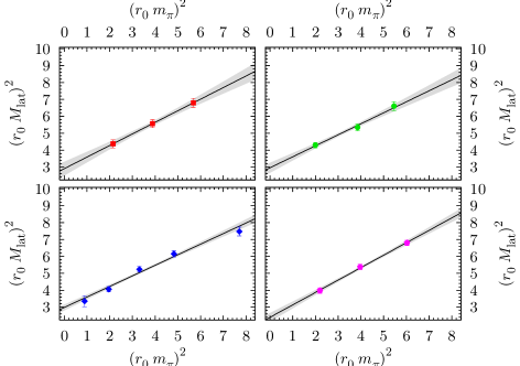
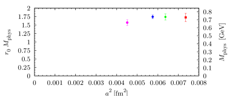
Figure 9: Scaling test: the upper plots show extrapolations as in Fig. 3 for each $\beta$ separately. The lower plot shows the extrapolated values of the monopole mass at the corresponding square of the lattice spacing.

6 Conclusion

We have calculated the electromagnetic form factor of the pion, using lattice configurations generated by the QCDSF/UKQCD collaboration with two flavours of dynamical, $O(a)$ improved Wilson fermions. The corresponding pion masses range from 400 to 1180  MeV. The momentum dependence of the pion form factor was studied up to $Q^{2}$ around $4{\,\text{Ge}\kern-0.66666pt\text{V\/}}^{2}$. Within errors, the pion form factor is described very well by a monopole form (20) in this range, for all our lattice pion masses. A linear chiral extrapolation to the physical pion mass leads to a monopole mass of $M=0.727(16){\,\text{Ge}\kern-0.66666pt\text{V\/}}$. This corresponds to a squared charge radius $\langle r^{2}\rangle=0.441(19)~{}\text{fm}^{2}$, in good agreement with experiment. Our extrapolated lattice data for the form factor is compared with experimental measurements in Fig. 4. Other lattice results are quoted in Table 6.

The large parameter space of the gauge configurations we used makes it possible to explore artifacts arising from the finite lattice spacing and volume. An empirical fit allowing for a volume dependence leads to an increase of the monopole mass by 3% at infinite volume and the physical point. Within errors, our results show no clear dependence on the lattice spacing in the range $a=\text{0.07~{}--~{}0.11~{}fm}$ of our simulations. Including estimates for systematical errors, our final result then is $M=0.727\pm 0.016\,(\text{stat})\pm 0.046\,(\text{syst})+0.024\,(\text{vol}){\,\text{Ge}\kern-0.66666pt\text{V\/}}$, which translates to a charge radius of $\langle r^{2}\rangle=0.441\pm 0.019\,(\text{stat})\pm 0.056\,(\text{syst})-0.029\,(\text{vol})~{}\text{fm}^{2}$. The first error is purely statistical, followed by a systematic uncertainty due to the ansatz for the fitting function and the extrapolation to physical pion masses (for which we added in quadrature the errors $\Delta M_{\text{ext}}$ and $\Delta M_{\text{fit}}$ obtained in Section 5.1). The last error reflects a possible shift because of finite volume effects as just discussed. We have set the scale using the Sommer parameter with $r_{0}=0.467$ fm. We note that the analysis leading to our result for $M$ is independent of the scale setting, so that a different value of $r_{0}$ would lead to a simple rescaling of the above values.

Table 6: An overview of lattice results for the pion charge radius along with the experimental value. We only quote results that are extrapolated to the physical point. The quoted lattice errors are purely statistical.

$\langle r^{2}\rangle$ [fm2]	type of result	Reference
0.452(11)	experimental value	PDG 2004 [24]
0.441(19)	Clover improved Wilson fermions, $N_{f}=2$	this work
0.396(10)	Clover improved Wilson fermions, $N_{f}=2$	JLQCD [9]
0.37(2)	Wilson fermions, quenched	[5]
0.310(46)	hybrid ASQTAD/DWF, $N_{f}=2+1,3$	LHPC [8]

References

- [1] QCDSF and UKQCD Collaboration, D. Brömmel et al., Proc. Sci. LAT2005, (2005) 360, hep-lat/0509133.
- [2] G. Martinelli and C. T. Sachrajda, Nucl. Phys. B306, (1988) 865.
- [3] T. Draper, R. M. Woloshyn, W. Wilcox, and K.-F. Liu, Nucl. Phys. B318, (1989) 319.
- [4] Bern-Graz-Regensburg (BGR) Collaboration, S. Capitani, C. Gattringer, and C. B. Lang, Phys. Rev. D73, (2006) 034505, hep-lat/0511040.
- [5] J. van der Heide, J. H. Koch, and E. Laermann, Phys. Rev. D69, (2004) 094511, hep-lat/0312023.
- [6] A. M. Abdel-Rehim and R. Lewis, Phys. Rev. D71, (2005) 014503, hep-lat/0410047.
- [7] RBC Collaboration, Y. Nemoto, Nucl. Phys. Proc. Suppl. 129, (2004) 299, hep-lat/0309173.
- [8] LHP Collaboration, F. D. R. Bonnet, R. G. Edwards, G. T. Fleming, R. Lewis, and D. G. Richards, Phys. Rev. D72, (2005) 054506, hep-lat/0411028.
- [9] JLQCD Collaboration, S. Hashimoto et al., PoS LAT2005, (2006) 336, hep-lat/0510085.
- [10] S. Sint and P. Weisz, Nucl. Phys. B502, (1997) 251, hep-lat/9704001.
- [11] QCDSF-UKQCD Collaboration, T. Bakeyev et al., Phys. Lett. B580, (2004) 197, hep-lat/0305014.
- [12] S. Capitani et al., Nucl. Phys. Proc. Suppl. 73, (1999) 294, hep-lat/9809172.
- [13] QCDSF Collaboration, M. Göckeler et al., Phys. Rev. D71, (2005) 034508, hep-lat/0303019.
- [14] A. Ali Khan et al., (2006), hep-lat/0603028.
- [15] C. Aubin et al., Phys. Rev. D70, (2004) 094505, hep-lat/0402030.
- [16] C. Best et al., Phys. Rev. D56, (1997) 2743, hep-lat/9703014.
- [17] UKQCD Collaboration, C. R. Allton et al., Phys. Rev. D47, (1993) 5128, hep-lat/9303009.
- [18] NA7 Collaboration, S. R. Amendolia et al., Nucl. Phys. B277, (1986) 168.
- [19] H. P. Blok, G. M. Huber, and D. J. Mack, (2002), nucl-ex/0208011.
- [20] H. Ackermann et al., Nucl. Phys. B137, (1978) 294.
- [21] P. Brauel et al., Zeit. Phys. C3, (1979) 101.
- [22] The Jefferson Lab Collaboration, V. Tadevosyan et al., (2006), nucl-ex/0607007. The Jefferson Lab -2 Collaboration, T. Horn et al., (2006), nucl-ex/0607005.
- [23] The Jefferson Lab Collaboration, J. Volmer et al., Phys. Rev. Lett. 86, (2001) 1713, nucl-ex/0010009.
- [24] Particle Data Group Collaboration, S. Eidelman et al., Phys. Lett. B592, (2004) 1.
- [25] T. B. Bunton, F. J. Jiang, and B. C. Tiburzi, Phys. Rev. D74, (2006) 034514.
- [26] J.-W. Chen, W. Detmold, and B. Smigielski, (2006), hep-lat/0612027.
- [27] B. Borasoy and R. Lewis, Phys. Rev. D71, (2005) 014033, hep-lat/0410042.
- [28] M. Guagnelli and R. Sommer, Nucl. Phys. Proc. Suppl. 63, (1998) 886, hep-lat/9709088.
- [29] M. Göckeler et al., Phys. Rev. D73, (2006) 014513, hep-ph/0502212.
- [30] UKQCD Collaboration, C. R. Allton et al., Phys. Rev. D65, (2002) 054502, hep-lat/0107021.