Fixed twist dynamics of $SO(3)$ Gauge Theory

Abstract

We perform a throughout study of 3+1 dim. $SO(3)$ LGT for fixed-twist background. We concentrate in particular on the physically significant trivial and 1-twist sectors. Introducing a $\mathbb{Z}_{2}$ monopole chemical potential the 1^st order bulk transition is moved down in the strong coupling region and weakened to 2^nd order in the 4-dim Ising model universality class. In this extended phase diagram we gain access to a confined phase in every fixed twist sector of the theory. The Pisa disorder operator is employed together with the Polyakov loop to study the confinement-deconfinement transition in each sector. Due to the specific properties of both operators, most results can be used to gain insight in the ergodic theory, where all twist sectors should be summed upon. An explicit mapping of each fixed twist theory to effective positive plaquette models with fixed twisted boundary conditions is applied to better establish their properties in the different phases.

1 Introduction

It is common knowledge from lattice investigations that Yang-Mills theories possess a finite temperature transition from a confined to a deconfined phase [1, 2] linked to the spontaneous breaking of center symmetry [3, 4]. For $SU(2)$ such transition is 2^nd order and therefore in the universality class of Ising 3-d [5]. The alleged preferential rôle that the discretization in the fundamental representation plays in such result has been widely discussed in the literature (see e.g. [6]).

The difficulties connected to the use of the adjoint discretization, which according to universality should deliver the same results as the fundamental one for the observables which have a common representation, have been widely discussed and partially understood for a long time [7, 8, 9, 10]: the theory exhibits a bulk transition along the adjoint coupling linked to the condensation of $\mathbb{Z}_{2}$ magnetic monopoles, whose Dirac strings correspond to open $\mathbb{Z}_{2}$ magnetic vortices; at the same time it was pointed out how the introduction of ad-hoc chemical potentials could affect the phase diagram and give access to the continuum limit in the weak coupling phase [9, 10, 11]. Interestingly enough, such topological defects proved also to be the key to understand a further property of the adjoint discretization: in the phase where $\mathbb{Z}_{2}$ monopoles condense the $SO(3)$ partition function with periodic boundary conditions (b.c.) should be equivalent to the sum of $SU(2)$ partition functions with all possible twisted b.c. [12, 13, 14]. In the center blind adjoint discretization maximal ’t Hooft loops are therefore physical topological excitations rather than boundary constraints as in the fundamental one [12, 14, 15]. First attempts to simulate the modified pure adjoint theory proposed in [9, 10, 11] were performed in [16, 17, 18, 19, 20]. Due to the absence of a suitable order parameter the authors had to rely on thermodynamic quantities, making the study of the finite temperature phase transition and its continuum limit quite demanding [20]. Moreover, it was observed that for small chemical potential and on top of the bulk transition the theory exhibits states where the adjoint Polyakov loop $L_{A}=-1/3$ [16, 18]. In [15] it was pointed out how such phase actually corresponds to the non trivial twist sectors of the theory upon which the partition function should be summed, the analysis in Ref. [20] neglecting such aspect. High barriers in the weak coupling phase among such different topological sectors make an ergodic sampling of the partition function very difficult already for small volumes [15], leaving the problem of the behaviour of the full adjoint theory open. It was only recently that consistent efforts through parallel tempering have led to first results in the ergodic theory [21, 22, 23].

In a series of papers [24, 25, 26, 27, 28, 29] the analysis of the trivial twist sector was developed by studying the spatial distribution of the fundamental Polyakov loop $L_{F}$ [26] and the Pisa disorder operator [28]. In this paper we will refine and extend such results to the $SO(3)$ dynamics of both trivial and non-trivial twist sectors. In particular, in [15] it was argued that any configuration generated by an adjoint weight at fixed twist could be “gauge fixed” to a configuration kinematically equivalent to a fundamental positive plaquette model [30] with corresponding twisted b.c.; whether a corresponding effective action can be written is however an open question. In Sec. 3 for each fixed twist sector an explicit mapping to such positive plaquette model configurations will be given. This enables us to define a non-vanishing $L_{F}$ and determine the properties of the deconfinement phase transition at fixed twist with “standard” methods. The intrinsic limitations of such procedure will be also discussed. The interest of our extensive fixed twist analysis will be made clear in Sec. 4: fixed twist results can deliver “low cost” informations about the ergodic behaviour of some observables in regimes hard to investigate with the full $SO(3)$ partition function [22, 23].

2 Action and observables

We shall study the adjoint Wilson action modified by a $\mathbb{Z}_{2}$ monopole suppression term:

$$S=\beta_{A}\sum_{P}\left(1-\frac{\mathrm{Tr}_{A}U_{P}}{3}\right)+\lambda\sum_{c}(1-\sigma_{c})\,,$$ (1)

where $U_{P}$ denotes the standard plaquette and $\mathrm{Tr}_{A}=2\mathrm{Tr}_{F}^{2}$ - 1. The product $\sigma_{c}=\prod_{P\in\partial c}\mathrm{sign}(\mathrm{Tr}_{F}U_{P})$ taken around all $N_{c}$ elementary 3-cubes $c$ defines the $\mathbb{Z}_{2}$ magnetic charges. Action (1) is center-blind in the entire $\beta_{A}-\lambda$ plane (Fig. 1) [26].

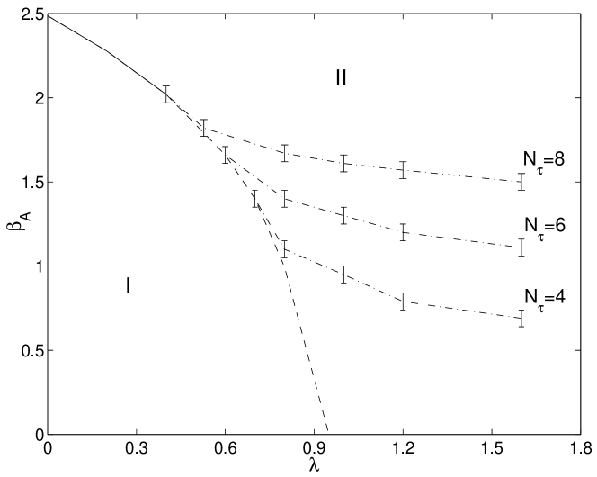
Figure 1: $\beta_{A}-\lambda$ plane. The bulk transition is shown together with the finite temperature lines as found at trivial twist in [26, 28]

The density $M=1-\langle\frac{1}{N_{c}}\sum_{c}\sigma_{c}\rangle$ tends to one in the strong coupling region (phase I) and to zero in the weak coupling limit (phase II). In the $(\lambda,\beta_{A})$ plane such phases are separated by a bulk phase transition whose order weakens from the strong 1^st order at $\lambda=0$, $\beta_{A}\simeq 2.5$ to 2^nd as $\lambda$ increases [9, 20, 26]. For low $\beta_{A}$ the theory can be shown to be dual to a 4-d Ising model [9], the bulk line terminating at $\lambda\simeq 0.92$.

As already anticipated, maximal ’t Hooft loops can be generated dynamically in such adjoint theory, since periodic b.c. on the adjoint fields automatically include all twisted b.c. for their fundamental representatives. Appropriate twist observables can be introduced through

$$z_{\mu\nu}\equiv\sum_{\rho\sigma}\frac{1}{N_{\rho}N_{\sigma}}\prod_{P\;\in\;\mathrm{plane}\;\mu\nu}\mathrm{signTr}_{F}U_{P}\,,\hskip 2.84544pt(\epsilon_{\rho\sigma\mu\nu}=1)\,.$$ (2)

Like the $\mathbb{Z}_{2}$ monopoles, such observables are center blind [15, 26]. In Ref. [13, 14] it was shown how the constraint $\sigma_{c}=1$, identically satisfied in phase II, assures that $z_{\mu\nu}$ in eq. (2) can only take the values $\pm 1$; moreover the partition function generated by action (1) should be equivalent to the sum of all partition functions generated with fundamental action and twisted b.c. Since at finite temperature the production of non trivial space like twists ($\mu$, $\nu\neq 4$) will be exponentially suppressed, we can concentrate on time like twists $z_{i4}$, ($i=1$, 2, 3). We will denote the different twist sectors $z$ simply by counting the number of non trivial twists in the various directions. Since as anticipated tunnelling among them is strongly suppressed, one simply needs to choose appropriate initial conditions and employ a local update algorithm (standard Metropolis) within phase II to keep the twist sectors fixed.

A further observable which can be measured at fixed twist is the Pisa disorder operator [31], motivated by the dual superconductor scenario for the QCD vacuum [32, 33, 34]. Its construction in the case of the $SO(3)$ at non trivial twist follows the same lines as in the trivial twist case [28]. The magnetically charged operator $\mu$ shifts the quantum field at a given time slice by a classical external field corresponding to an Abelian monopole, with the $U(1)$ subgroup of the gauge group, which defines the magnetic charge, selected by an Abelian projection usually fixed by diagonalizing an operator $X$ in the adjoint representation. As in Ref. [28] we will work with the random Abelian projection (RAP) introduced in Ref. [35].

The disorder parameter is defined as

$$\langle\mu(t)\rangle=\frac{\int(DU)_{M}e^{-S_{M}(t)}}{\int(DU)e^{-S}}\,,$$ (3)

where $S_{M}(t)$ denotes the Wilson action with the space-time plaquettes $U_{i4}(\vec{x},t)$ at a fixed time-slice $t$ modified by an insertion of an external monopole field

$$\widetilde{U}_{i4}(\vec{x},t) = U_{i}(\vec{x},t)\Phi_{i}(\vec{x}+\hat{i},\vec{y})U_{4}(\vec{x}+\hat{i},t)\times$$ (4)

$$\times U_{i}^{\dagger}(\vec{x},t+1)U_{4}^{\dagger}(\vec{x},t))\,,$$

where $\Phi_{i}(\vec{x},\vec{y})=\Omega e^{iT_{a}b^{a}_{i}(\vec{x}-\hat{i},\vec{y})}\Omega^{\dagger}$, with $\Omega$ the gauge transformation which diagonalizes the operator $X$. $T_{a}$ denote the generators of the Cartan subalgebra and $\vec{b}$ the discretized transverse field generated at the lattice spatial point $\vec{x}$ by a magnetic monopole sitting at $\vec{y}$. It should be stressed that only the plaquette contribution to the action (1) is modified by the insertion of the monopole field and not the chemical potential term $\lambda$. From the definition of $\mu$ it can be shown that a monopole field is added at time slice $t+1$ by using a suitable change of variable. Iterating the procedure it can be proved that $\mu$ effectively corresponds to an operator which at time slice $t$ creates a monopole propagating forward in time until it is annihilated by an antimonopole at $t+\Delta t$. The correlation function $D(\Delta t)=\langle\bar{\mu}(\vec{y},t+\Delta t)\mu(\vec{y},t)\rangle$ describes the creation of a monopole at $(\vec{y},t)$ and its propagation from $t$ to $t+\Delta t$. At large $\Delta t$, by cluster property $D(\Delta t)\simeq A\exp(-M\Delta t)+\langle\mu\rangle^{2}$. $\langle\mu\rangle\neq 0$ indicates spontaneous breaking of the $U(1)$ magnetic symmetry and hence dual superconductivity. In the thermodynamic limit one expects $\langle\mu\rangle\neq 0$ for $T<T_{c}$, while $\langle\mu\rangle=0$ for $T>T_{c}$, if the deconfining phase transition is associated with a transition from a dual superconductor to the normal state. At finite temperature there is no way to put a monopole and an antimonopole at large distance along the $t$-axis as it is done at $T=0$, since at $T\sim T_{c}$ the temporal extent $N_{\tau}a$ is comparable to the correlation length. Therefore, one measures directly $\langle\mu\rangle$ but with $C^{*}$-periodic b.c. in time direction imposed to the numerator in Eq. (3) in order to ensure magnetic charge conservation, $U_{i}(\vec{x},N_{\tau})=U_{i}^{*}(\vec{x},0)$, where $U_{i}^{*}$ is the complex conjugate of $U_{i}$, in the following indicated by a suffix $M$ in the observables. They effectively create a dislocation with magnetic charge -1 at the boundary which annihilates the positive magnetic charge created by the operator $\mu$. An analogous condition holds also for link variables defined in the adjoint representation, i.e. $U_{i}(\vec{x},N_{\tau})=(\mathbb{I}_{3}+2T^{2}_{2})U_{i}(\vec{x},0)(\mathbb{I}_{3}+2T^{2}_{2})$; charge conjugation is realized in both representations through rotations by an angle $\pi$ around the color 2-axis. The adjoint representation makes moreover clear how $C^{*}$ b.c. are up to a gauge transformation equivalent to twisted b.c. and therefore “natural” in our adjoint theory.

A technical difficulty is that, since $\langle\mu\rangle$ is the average of the exponential of a sum over the physical volume, it is affected by large fluctuations which make it difficult to measure in Monte Carlo simulations. A way out is to compute the derivative with respect to the coupling parameter $\beta$ (i.e. $\beta_{A}$) $\rho=\frac{d}{d\beta}\log\langle\mu\rangle=\langle\Pi\rangle_{S}-\langle\Pi_{M}\rangle_{S_{M}}$, which yields all the relevant informations on $\mu$. It is the difference between the Wilson plaquette action term $\Pi$ averaged with the usual measure and the modified plaquette action term $\Pi_{M}$ averaged with the modified measure $(DU)_{M}e^{-S_{M}}/\int(DU)_{M}e^{-S_{M}}$. The order parameter itself can in principle be reconstructed from $\langle\mu\rangle=\exp\left(\int_{0}^{\beta}\rho(\beta^{\prime})d\beta^{\prime}\right)$. $\rho$ should vanish in the thermodynamical limit for $\beta<\beta_{c}$ if $\langle\mu\rangle\neq 0$. A sharp negative peak for $\rho$ diverging in the thermodynamical limit should signal a phase transition associated with the restoring of the dual magnetic symmetry, while above $T_{c}$ $\rho$ should show negative plateaus diverging with the volume to ensure $\langle\mu\rangle=0$.

3 Symmetry transformation

The absence of a “cheap” order parameter like $L_{F}$ has been one of the major obstacles in determining the properties of $SO(3)$ at fixed twist [20, 26, 28]. We solve here this problem by explicitly constructing the mapping suggested in Ref. [15] between the $SO(3)$ theory at fixed twist and configurations classified by some positive plaquette model [30]. The constraint $\sigma_{c}=1$ identically satisfied in phase II is key for the existence of such mapping: in spite of the center blindness of action (1), it makes the signs of the fundamental plaquettes no more completely random. A further constraint is given by the value of $z_{\mu\nu}$, where all parallel planes concurring to it in eq. 2 must be equal due to the $\sigma_{c}=1$ condition. In the case of trivial twist, for example, this will force first of all every 3-cube to have an even number of negative plaquettes, which will therefore be either parallel or will have a link in common. Furthermore, every 2-d plane must also have an even number of negative plaquettes. Therefore, the allowed configurations must consist of a superposition of two possible situation: an even number of negative stacks of plaquettes $P_{\mu\nu}$ in all parallel planes $\mu\nu$; or a set of negative plaquettes $P_{\mu\nu}$, $P_{\mu\rho}$ joined by a common link $U_{\mu}$, which must always occur in pairs in both ${\mu\nu}$ and ${\mu\rho}$ planes. In the case of non-trivial twist the situation is similar, with the only difference that the number of negative plaquettes in certain planes will now be odd.

As an illustration, take a configuration arising from a simulation at $N_{s}=N_{\tau}=4$ (Fig. 2 (a-c), Fig. 3 (a-c)). By flipping the sign of a generic link six plaquettes will be affected while obviously $\sigma_{c}$ and $z_{\mu\nu}$ will remain unchanged. One can therefore start to sweep the whole lattice changing first the sign of some links so to make all plaquettes in the $xy$ plane positive (Fig. 2 (d-f), Fig. 3 (d-f)). One can now proceed with a second sweep which makes all plaquettes in the $xz$ plane positive by leaving the $xy$ untouched, i.e. by flipping only $z$ and $t$ links. Fig. 2 (g-i), Fig. 3 (g-i) now illustrate clearly the situation: only pairs of plaquettes which can be made positive by a $t$ link flip are present. For non trivial twist the procedure will be the same, with the only difference that of course at the end a stack of plaquettes ensuring $z_{\mu\nu}=-1$, i.e. twisted b.c., must remain. Such procedure provides us with a kinematic identification of adjoint configurations with a positive plaquette model (with periodic or twisted b.c.); it is not a dynamical mapping to a positive plaquette action of the type given in Ref. [30], since we still generate our fields with an adjoint center-blind weight. In some sense it amounts to a “gauge fixing” which removes the local $\mathbb{Z}_{2}$ freedom intrinsic to the adjoint weight; another choice, e.g. all negative plaquettes, could have been equally made. Since no dynamical identification is possible, the positive plaquette fields we obtain will not be identical to the one generated through the action given in Ref. [30]. They might however exhibit similar scaling properties. For each configuration generated in the MC with weight given by eq. 1 we have applied the above algorithm to obtain a configuration where fundamental observables do not vanish identically when averaged over the volume, although they should be interpreted as gauge dependent observables in a gauge fixed theory.

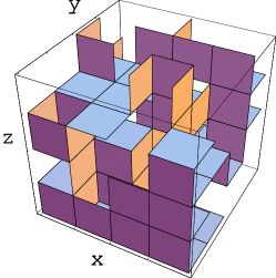
(a) $xyz$ at ${t}=1$

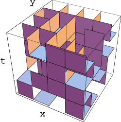
(b) $xyt$ at ${z}=1$

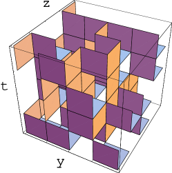
(c) $yzt$ at ${x}=1$

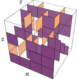
(d) $xyz$ at ${t}=1$

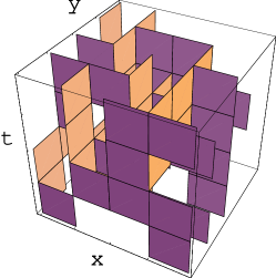
(e) $xyt$ at ${z}=1$

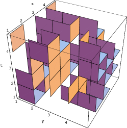
(f) $yzt$ at ${x}=1$

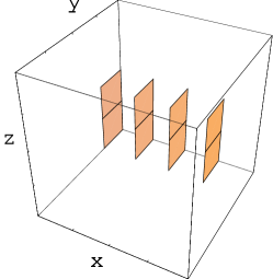
(g) $xyz$ at ${t}=1$

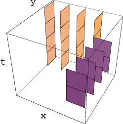
(h) $xyt$ at ${z}=1$

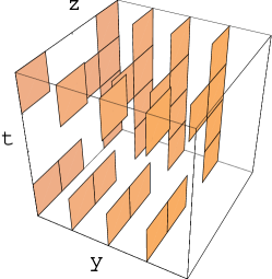
(i) $yzt$ at ${x}=1$

Figure 2: Suppression of the negative plaquettes in the trivial twist sector.

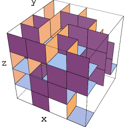
(a) $xyz$ at ${t}=1$

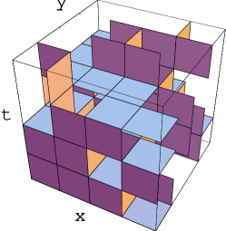
(b) $xyt$ at ${z}=1$

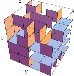
(c) $yzt$ at ${x}=1$

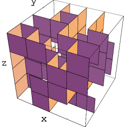
(d) $xyz$ at ${t}=1$

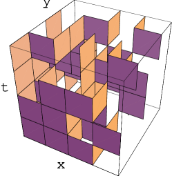
(e) $xyt$ at ${z}=1$

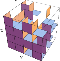
(f) $yzt$ at ${x}=1$

(g) $xyz$ at ${t}=1$

(h) $xyt$ at ${z}=1$

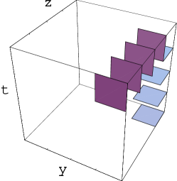
(i) $yzt$ at ${x}=1$

Figure 3: Suppression of the negative plaquettes in the non-trivial twist sector.

We can now measure $L_{F}$ and its susceptibility in all fixed twist sectors of the adjoint theory and use it as an order parameter to determine the critical exponents. Although in Ref. [36] an alternative definition of $L_{F}$ modified via a twist eater at the boundary has been used for the fundamental theory with fixed twisted b.c., we have chosen to stick to the standard definition for a number of reasons. From a purely formal point of view, for the full adjoint theory reflection positivity can only be invoked for adjoint Polyakov loop correlators, ensuring their positivity irrespective of the twist sector; in other words such quantities are invariant also under large, twist changing gauge transformations and should be considered the “fundamental” ones. Since we wish to maintain the property $\mathrm{Tr}_{A}=2\mathrm{Tr}_{F}^{2}-1$ also for the local Polyakov loop $L(\vec{x})=\prod_{t=0}^{N_{\tau}}U_{4}(\vec{x},t)$, so to keep the volume average of $L_{A}$ proportional to the second moment of the spatial distribution of $L_{F}$, to ensure the correct behaviour under gauge transformations we are forced to keep the standard definition of $L_{F}$. From a practical point of view, our algorithm does not pick a particular representative of the homotopy class ensuring the fixed b.c. corresponding to the twist sector chosen. One would need to further fix the single links throughout the lattice to have b.c. representable through some specific twist eater at the boundary. The definition in Ref. [36] is therefore not easily applied to configurations derived from an adjoint weight at fixed twist sector. We think however that there is no real problem underlying such ambiguity, since measuring $L_{F}$ at non trivial twist is anyway an unphysical procedure. No fermion fields, not even in the limit of infinite mass, can be present with twisted b.c., so that no real physical interpretation can be given to $L_{F}$ and its correlators at non trivial twist.

4 Fixed twist vs. ergodic simulations

For the adjoint theory in phase II, being the twist sectors $z$ well defined, the ergodic expectation value of any observable $O$ can be always re-expressed through:

$$\langle O\rangle_{erg}=\frac{\sum_{i=0}^{3}\langle O\rangle|_{z={i}}Z_{SO(3)}|_{z={i}}}{\sum_{i=0}^{3}Z_{SO(3)}|_{z={i}}}\,,$$ (5)

where $\langle O\rangle|_{z={i}}$ is the expectation value of the observable restricted to the fixed twist sector $z=i$.

In general in absence of an ergodic algorithm the relative weights of the partition functions $Z_{SO(3)}|_{z={i}}$ remain unknown, although there is of course at least one case in which Eq. (5) is of use in a fixed twist analysis, namely when $\langle O\rangle|_{z={i}}\simeq\langle O\rangle$ $\forall i$, i.e. the observable is independent of the twist sector; in such case it will obviously be $\langle O\rangle_{erg}\simeq\langle O\rangle$.

The ratio of partition functions could in principle be estimated from the behaviour of the vortex free energy [12, 14, 37, 38, 36, 39], leading to

$$\frac{Z_{SO(3)}|_{z={i}}}{Z_{SO(3)}|_{z={j}}}\simeq c_{ij}$$ (6)

in the confined phase, while in the (deep) deconfined phase $T>>T_{c}$

$$\frac{Z_{SO(3)}|_{z={i}}}{Z_{SO(3)}|_{z={j}}}\simeq c_{ij}e^{-\frac{\tilde{\sigma}N_{s}^{2}}{T}(i-j)}\,,$$ (7)

$N_{s}$ being the spatial length of the lattice, $\tilde{\sigma}$ the dual string tension and the coefficients $c_{ij}$ taking the values

$$c_{ji} = c_{ij}^{-1};\;c_{ii}=1;\;c_{10}=c_{20}=3;\;$$

$$c_{21} = c_{30}=1;\;c_{31}=c_{32}=\frac{1}{3}\,.$$ (8)

This is quite straightforward to see: being the action cost to create $(i-j)$ maximal ’t Hooft loops strictly zero in $SO(3)$, the free energy to tunnel twist sector from $i$ to $j$ will simply be given by the entropy change

$$\Delta F_{ij}=-T\Delta S_{ij}=-T\log{\frac{Z_{SO(3)}|_{z={i}}}{Z_{SO(3)}|_{z={j}}}}\,.$$ (9)

This on the other hand will be dictated in the deconfined (confined) phase by an area (perimeter) law through the dual string tension, i.e. $\Delta F_{ij}=0$ for $T<T_{c}$ and $\Delta F_{ij}=T\tilde{\sigma}N_{s}^{2}(i-j)$ for $T>>T_{c}$. The factors $c_{ij}$ are due to the counting of states on a 3-torus topology, as indeed the existence of twists states with $z>1$ in the first place. In other words, on $T^{3}\times S^{1}$ there is one $z=0$ twist state, three independent $z=1$ and $z=2$ states and one $z=3$ state, while on $S^{3}\times S^{1}$ there is only one $z=0$ and one $z=1$ twist state.

In the thermodynamic limit $N_{s}\to\infty$ all twist states should therefore be equivalent in the confined phase with

$$\langle O\rangle_{erg}=\frac{\sum_{i=0}^{3}\langle O\rangle|_{z={i}}c_{i0}}{8}$$ (10)

while all the non-trivial ($z>0$) states will be exponentially suppressed above $T_{c}$ with

$$\langle O\rangle_{erg}=(1+e^{-\frac{\tilde{\sigma}N_{s}^{2}}{T}})^{-3}\sum_{i=0}^{3}\langle O\rangle|_{z={i}}c_{i0}e^{-\frac{\tilde{\sigma}N_{s}^{2}}{T}i},$$ (11)

so that if the $\langle O\rangle|_{z={i}}$ are bounded (or diverge less than exponentially) for $N_{s}\to\infty$ then obviously $\langle O\rangle_{erg}\simeq\langle O\rangle|_{z={0}}$. This will hold of course if $\langle O\rangle|_{z={i}}\simeq 0$ $\forall i\neq 0$.

There are however some difficulties with this standard picture. The vanishing of the dual string tension is just a sufficient and not a necessary condition for the existence of a confined phase, which on the other hand only assures that the deconfined behaviour in the regime $T>>T_{c}$ will necessarily obey eq. (11). No result was actually available in the literature for the confined phase of the ergodic $SO(3)$ until the studies in [21, 22, 23] appeared, which however point to a different behaviour of the center blind adjoint discretization from the fundamental one. We will therefore avoid to use eq. (10) in the interpretation of the results. This will however turn out not to be a major problem, most observable of interest resulting independent of the twist sector below $T_{c}$.

5 Results

5.1 The Pisa disorder operator

The analysis of $\rho$ in the trivial twist sector has already been carried out in Ref. [28] for different $N_{\tau}$. In Fig. 4(a) we show the behaviour of $\rho$ for chemical potential $\lambda=1.0$ at $N_{\tau}=4$ in the non trivial twist sector. The similarities with the trivial twist case end with the peak which should signal the transition ($\beta_{A}^{c}$ = 0.95). Above $\beta_{A}^{c}$ $\rho$ vanishes, in contrast to the strong diverging plateaus seen at trivial twist [28]. The transition at non trivial twist therefore cannot correspond, strictly speaking, to a deconfined phase. We shall try to better understand this through the analysis of other observables.

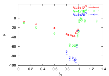
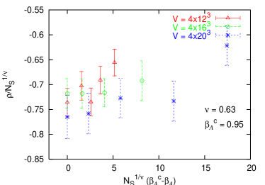
Figure 4: $\rho$ computed in the non trivial twist sector at finite temperature ($N_{\tau}=4$) for different values of the spatial volume and (a). Finite-size scaling analysis for $\rho$ (b).

A consistency FSS analysis taking the value $\beta_{A}^{c}=0.95$ and the critical exponents of the 3-d Ising model is shown in Fig. 4(b). We will comment on its quality in Sec. 5.2. One thing we would like to stress here is that such vanishing of $\rho$ poses no problem in the ergodic theory. Given the behaviour at trivial twist, eq. 11 ensures us that the Pisa disorder parameter will indicate deconfinement at high $\beta$, provided that there exists a diverging peak at some $\beta_{A}^{c}$. Since the peaks in the trivial and non trivial twist sector occur at slightly different $\beta_{A}^{c}$ ($\beta_{A}^{c}=0.98$ for $z=0$, cfr. [28] and the following section), this latter question can only be answered by a full ergodic simulation [23]. The situation at low $\beta$ is slightly more complicated. Although in all twist sectors $\rho$ assumes a constant bounded small negative value $\rho\simeq-k$ (cfr. [28]), therefore indicating $\langle\mu\rangle\neq 0$ also for the full ergodic theory, i.e. condensation of monopoles and confinement in the low $\beta$ region, the fact that it does not seem to strictly vanish in the thermodynamic limit might pose a conceptual problem: for every fixed $N_{\tau}$ $\langle\mu\rangle$ can be redefined post-hoc to assume a constant value through $exp(k\beta_{A}^{c}(N_{\tau}))$, but this rescaling factor will necessarily diverge for $SU(N)$ like $N_{\tau}^{\alpha k}$, up to logarithmic corrections depending on the higher order coefficients of the $\beta$-function, with $\alpha=2\beta_{0}(N^{2}-1)/N$, $\beta_{0}$ being its first coefficient. This might on the other hand be a conceptual obstacle in defining $\langle\mu\rangle$ in the continuum limit $N_{\tau}\to\infty$, although $\alpha$ is just $\simeq 1.4$ for $SU(2)$.

5.2 $L_{F}$ and the interquark potential

Fig. 5 (a, b) show the behaviour of $L_{F}$ and its susceptibility in the trivial twist sector after the mapping to the positive plaquette model at $\lambda=1.0$ for $N_{\tau}=4$. In Fig. 6 (a, b) we perform a FFS analysis with the Ising 3-d critical exponents and our best estimate $\beta_{A}^{c}=0.98$, which agrees with the result in Ref. [28] obtained through $\rho$.

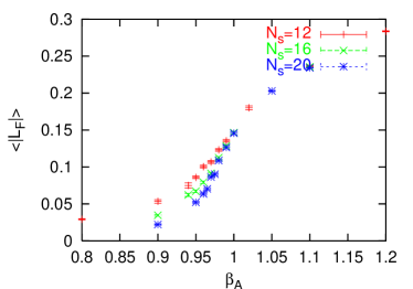
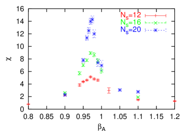
Figure 5: $L_{F}$ (a), its susceptibility $\chi$ (b).

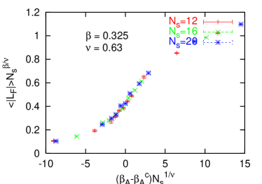
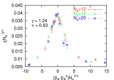
Figure 6: Quality of scaling for $L_{F}$ (a) and for $\chi$ (b).

This is confirmed in Fig. 7 (a, b), which show $L_{F}$ and $\chi$ at $\lambda=1.0$ for $N_{\tau}=6$. Again, our results are in agreement with the estimate $\beta_{A}^{c}=1.19$ from $\rho$ in Ref. [28].

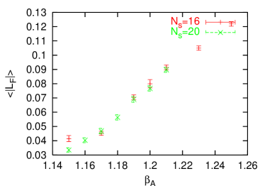
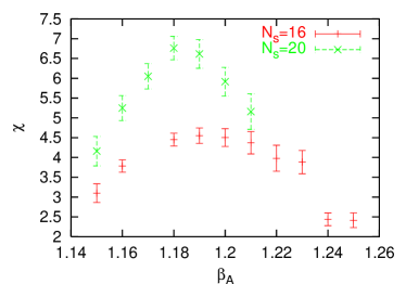
Figure 7: $L_{F}$ (a) and its susceptibility (b).

The non trivial twist sector offers more material for discussions. Fig. 8 (a,b) show $L_{F}$ and $\chi$ at $\lambda=1.0$ for $N_{\tau}=4$. $L_{F}$ rises at first above the “transition” (with $L_{A}$ also positive) to then tend to zero in the high $\beta_{A}$ limit, as expected from the known behaviour $L_{A}\to-1/3$. Such behaviour is not that of a standard deconfining theory, due to the non trivial background introduced by the non trivial twist. The determination of $\beta_{A}^{c}$ is more difficult, our best estimate remaining thus that from $\rho$ obtained in Sec. 5.1. In light of such problems and given the worse signal to noise ratio at non trivial twist the comparison of Fig. 4(b) with the scaling figures for $\rho$ in Ref. [28] is not bad. Compare also such result with the indubitably better scaling obtained here in Fig. 6 to have a measure of the intrinsic difficulties in performing precision measurements with $\rho$.

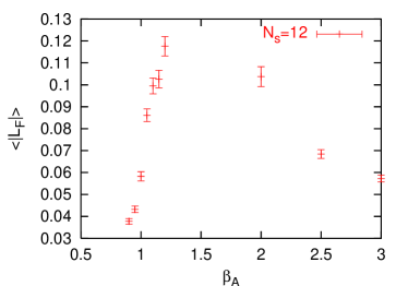
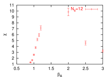
Figure 8: $L_{F}$ (a) and its susceptibility (b) in the non-trivial twist sector.

Figs. 9, 10 illustrate perhaps better the situation. There we have calculated the interquark potential from $L_{F}$ correlators at $\lambda=1.0$, $N_{\tau}=4$, $N_{s}=16$ for both twist sectors at various temperatures as a function of the distance. We have chosen to keep lattice units throughout since contrary to the fundamental case no result exists for the non perturbative scaling of adjoint models, e.g. through precision measurements of the string tension. Below $T_{c}$ (upper curve in both Figures) both trivial and non trivial twist show still a (slowly) linearly growing potential . The growth of $V(r)$ is moderate as expected, since the string tension should get dampened like $\sigma(T)=\sigma\sqrt{1-T^{2}/T_{c}^{2}}$ when approaching a 2^nd order transition, i.e. roughly by a factor 60$\%$ at the value $T=0.92T_{c}$ chosen. Above $T_{c}$ the situation changes. In the trivial twist case the long range interactions die very fast above $T_{c}$, having disappeared at $T\simeq 2T_{c}$, which corresponds to a lattice spacing roughly the half of that at $T_{c}$. In the non trivial sector however they persist quite consistently, so that it is not clear whether one can speak of deconfinement in the common understanding. The long range interactions are minimal (in lattice units) at $T\simeq 2T_{c}$, roughly coinciding with the peaks in $L_{F}$ and its susceptibility, to rise then again: at $T\simeq 4T_{c}$ (which corresponds to 25$\%$ of the $T_{c}$ lattice spacing) they have a similar strength in lattice units as at $T\simeq T_{c}$. Of course finite volume effects will start to be considerable at such relatively high $\beta_{A}$ values, so that a full analysis would imply going at much bigger $N_{s}$. The difference in qualitative behaviour between Fig. 9 and 10 remains anyway striking.

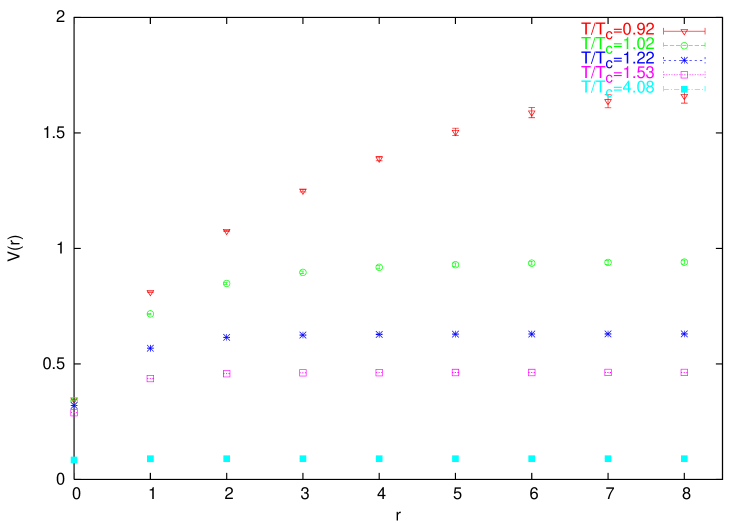
Figure 9: $q-\bar{q}$ potential from $L_{F}$ correlators at trivial twist.

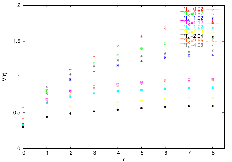
Figure 10: $q-\bar{q}$ potential from $L_{F}$ correlators at non trivial twist.

To conclude, Fig. 11 shows (again in lattice units) the fundamental string tension estimates in both twist sectors from (fundamental) Creutz ratios at $T=0$ ($16^{4}$), $\lambda=1$ and $\beta_{A}=0.98$. Comparing with the value $a^{2}\sigma\simeq 0.140$ obtained in the fundamental case at $T=0$ for $\beta\simeq 2.29$, i.e. the coupling corresponding to $T_{c}$ for $N_{\tau}=4$, one has the impression that our positive plaquette model representation of the adjoint theory has no dramatic scaling discrepancies with the standard fundamental theory. It would be interesting to recheck these non-trivial twist results either with the standard Wilson action or with a genuine positive plaquette model, of course with twisted boundary condition in both cases. Also the alternative definition of $L_{F}$ given in Ref.  [36] would be worth to explore. To our knowledge, although twisted b.c. have been used in the literature, no comparable result to those given here is available.

Fixing a non trivial background through twist sectors leads then to theories which are not equivalent to the standard one. While having a similar dynamics below $T_{c}$ they will not show the standard deconfining behaviour at high temperature.

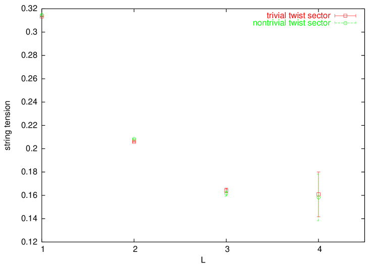
Figure 11: String tension estimate for $N_{s}=N_{\tau}=16$, $\beta_{A}=0.98$.

As discussed in section 3 there is of course a problem in the interpretation of the non trivial twist sector: even though as we have shown in the “confined” phase one can formally define an interquark potential and through it a fundamental string tension, there is actually no way to couple the gauge fields to fermions at finite temperature with twisted b.c. The twisted adjoint theory, contrary to the untwisted one, cannot therefore be considered equivalent to a standard fundamental Yang-Mills theory. $L_{F}$ and its correlators cannot therefore be related to the static potential of quarks. One should therefore not read much in their unusual behaviour.

6 Conclusions

In this paper we have studied the pure adjoint $SU(2)$ theory in the trivial and non-trivial twist sectors. We have been able to establish the properties of the different phases analyzing the Pisa disorder operator; through an explicit kinematic mapping to different positive plaquettes models with corresponding boundary conditions, we have also studied the behaviour of $L_{F}$. While the adjoint theory in the trivial twist sector can be considered equivalent to the standard $SU(2)$ gauge theory, the twisted theories show a quite different behaviour, in particular exhibiting no real deconfinement above $T_{c}$. In light of this, we are led to conclude that only the trivial twist sector and the full ergodic theory, i.e. summing over all twist sectors, can be considered good discretizations of Yang-Mills theories: the former gives the quenched theory, the second the full pure gauge case. However, many of our results here obtained for the fixed twisted case, through the considerations in Sec. 4, can be used to establish the properties of the ergodic theory in regimes where sampling the full partition function would be very expensive in computer time.

7 Acknowledgements

We thank A. Di Giacomo, L. Del Debbio, M. Müller-Preussker, M. D’Elia and P. de Forcrand for valuable comments and discussions. A special thank goes to Oliver Jahn for encouraging us to find the explicit mappings to positive plaquette models.

References

- [1] L. D. McLerran, B. Svetitsky, Phys. Lett. B98 (1981) 195.
- [2] J. Kuti, J. Polonyi, K. Szlachanyi, Phys. Lett. B98 (1981) 199.
- [3] A. M. Polyakov, Phys. Lett. B72 (1978) 477.
- [4] L. Susskind, Phys. Rev. D20 (1979) 2610.
- [5] B. Svetitsky, L. G. Yaffe, Nucl. Phys. B210 (1982) 423.
- [6] A. V. Smilga, Ann. Phys. 234 (1994) 1.
- [7] G. Bhanot, M. Creutz, Phys. Rev. D24 (1981) 3212.
- [8] J. Greensite, B. Lautrup, Phys. Rev. Lett. 47 (1981) 9.
- [9] I. G. Halliday, A. Schwimmer, Phys. Lett. B101 (1981) 327.
- [10] I. G. Halliday, A. Schwimmer, Phys. Lett. B102 (1981) 337.
- [11] L. Caneschi, I. G. Halliday, A. Schwimmer, Nucl.Phys.B200 (1982) 409.
- [12] G. ’t Hooft, Nucl. Phys. B153 (1979) 141.
- [13] G. Mack, V. B. Petkova, Zeit. Phys. C12 (1982) 177.
- [14] E. Tomboulis, Phys. Rev. D23 (1981) 2371.
- [15] P. de Forcrand, O. Jahn, Nucl. Phys. B651 (2003) 125.
- [16] S. Cheluvaraja, H. S. Sharathchandra, hep-lat/9611001.
- [17] S. Datta, R. V. Gavai, Phys. Lett. B392 (1997) 172.
- [18] S. Datta, R. V. Gavai, Phys. Rev. D57 (1998) 6618.
- [19] S. Datta, R. V. Gavai, Phys. Rev. D62 (2000) 054512.
- [20] S. Datta, R. V. Gavai, Phys. Rev. D60 (1999) 034505.
- [21] G. Burgio et al. , PoS LAT2005 (2006) 288.
- [22] G. Burgio et al., Phys. Rev. D74 (2006) 071502.
- [23] G. Burgio et al. , hep-lat/0610097.
- [24] A. Barresi, G. Burgio, M. Muller-Preussker, Nucl. Phys. Proc. Suppl. 106 (2002) 495.
- [25] A. Barresi, G. Burgio, M. Muller-Preussker, Nucl. Phys. Proc. Suppl. 119 (2003) 571.
- [26] A. Barresi, G. Burgio, M. Muller-Preussker, Phys. Rev. D69 (2004) 094503.
- [27] A. Barresi, G. Burgio, M. Muller-Preussker, Color confinement-Wako 2003 (2004) 82.
- [28] A. Barresi, G. Burgio, M. D’Elia, M. Mueller-Preussker, Phys. Lett. B599 (2004) 278.
- [29] A. Barresi, G. Burgio, M. Muller-Preussker, Nucl. Phys. Proc. Suppl. 129 (2004) 695.
- [30] J. Fingberg, U. M. Heller, V. K. Mitrjushkin, Nucl. Phys. B435 (1995) 311.
- [31] A. Di Giacomo, G. Paffuti, Phys. Rev. D56 (1997) 6816.
- [32] Y. Nambu, Phys. Rev. D10 (1974) 4262.
- [33] S. Mandelstam, Phys. Rev. D11 (1975) 3026.
- [34] G. ’t Hooft, Nucl. Phys. B79 (1974) 276.
- [35] J. M. Carmona, M. D’Elia, A. Di Giacomo, B. Lucini, G. Paffuti, Phys. Rev. D64 (2001) 114507.
- [36] P. de Forcrand, L. von Smekal, Phys. Rev. D66 (2002) 011504.
- [37] T. G. Kovacs, E. T. Tomboulis, Phys. Rev. Lett. 85 (2000) 704.
- [38] P. de Forcrand, M. D’Elia, M. Pepe, Phys. Rev. Lett. 86 (2001) 1438.
- [39] P. de Forcrand, D. Noth, Phys. Rev. D72 (2005) 114501.