Non-perturbatively Determined Relativistic Heavy Quark Action

Abstract

We present a method to non-perturbatively determine the parameters of the on-shell, $O(a)$-improved relativistic heavy quark action. These three parameters, $m_{0}$, $\zeta$, and $c_{B}=c_{E}$ are obtained by matching finite-volume, heavy-heavy and heavy-light meson masses to the exact relativistic spectrum through a finite-volume, step-scaling recursion procedure. We demonstrate that accuracy on the level of a few percent can be achieved by carrying out this matching on a pair of lattices with equal physical spatial volumes but quite different lattice spacings. A fine lattice with inverse lattice spacing $1/a=5.4$ GeV and $24^{3}\times 48$ sites and a coarse, $1/a=3.6$ GeV, $16^{3}\times 32$ lattice are used together with a heavy quark mass $m$ approximately that of the charm quark. This approach is unable to determine the initially expected, four heavy-quark parameters: $m_{0}$, $\zeta$, $c_{B}$ and $c_{E}$. This apparent non-uniqueness of these four parameters motivated the analytic result, presented in a companion paper, that this set is redundant and that the restriction $c_{E}=c_{B}$ is permitted through order $a|{\mathchoice{\!\stackrel{{\scriptstyle{}_{{}_{\>\scriptstyle\rightarrow}}}}{{\displaystyle p}}\!}{\!\stackrel{{\scriptstyle{}_{{}_{\>\scriptstyle\rightarrow}}}}{{\textstyle p}}\!}{\!\stackrel{{\scriptstyle{}_{{}_{\>\scriptscriptstyle\rightarrow}}}}{{\scriptstyle p}}\!}{\!\stackrel{{\scriptstyle{}_{{}_{\>\scriptscriptstyle\rightarrow}}}}{{\scriptscriptstyle p}}\!}}|$ and to all orders in $ma$ where ${\mathchoice{\!\stackrel{{\scriptstyle{}_{{}_{\>\scriptstyle\rightarrow}}}}{{\displaystyle p}}\!}{\!\stackrel{{\scriptstyle{}_{{}_{\>\scriptstyle\rightarrow}}}}{{\textstyle p}}\!}{\!\stackrel{{\scriptstyle{}_{{}_{\>\scriptscriptstyle\rightarrow}}}}{{\scriptstyle p}}\!}{\!\stackrel{{\scriptstyle{}_{{}_{\>\scriptscriptstyle\rightarrow}}}}{{\scriptscriptstyle p}}\!}}$ is the heavy quark’s spatial momenta.

I Introduction

The study of flavor physics and CP violation plays a central role in particle physics. In particular, many of the parameters of the Standard Model can be constrained by measurements of the properties of hadrons containing heavy quarks. However, to do this one needs theoretical determination of strong-interaction masses and matrix elements to connect the experimental measurements with those fundamental quantities. Lattice quantum chromodynamics (QCD) provides a first-principles method for the computation of these hadronic masses and matrix elements. However, lattice calculations with heavy quarks present special difficulties since in full QCD calculations, which properly include the effects of dynamical quarks, it is impractical to work with lattice spacings sufficiently small that errors on the order of $ma$ can be controlled. These problems are addressed by using a number of improved heavy quark actions designed to control or avoid these potentially important finite lattice spacing errors. The results of recent calculations of basic parameters of the Standard Model can be found in the lattice heavy quark reviews of Refs. Ryan (2002); Yamada (2003); Kronfeld (2004); Wingate (2005); Okamoto (2005).

A variety of fermion actions have been used in lattice calculations involving heavy quarks Mannel et al. (1992); Thacker and Lepage (1991); Lepage et al. (1992); Hashimoto and Matsufuru (1996); Sloan (1998); Foley and Lepage (2003). These include heavy quark effective theory (HQET) (for which the static approximation is the leading term) and non-relativistic QCD (NRQCD). These methods have significant limitations: NRQCD has no continuum limit, and although HQET has a continuum limit, it cannot be applied to quarkonia. While systems involving bottom quarks may permit a successful expansion in inverse powers of $m$, this is likely not true for systems including a charm quark.

A third approach, the one adopted here, is the Fermilab or relativistic heavy quark (RHQ) method El-Khadra et al. (1997); Aoki et al. (2003) in which extra axis-interchange asymmetric terms are added to the usual relativistic action. As is discussed below, this action can accurately describe heavy quark systems provided the improvement coefficients it contains are properly adjusted. As the heavy quark mass decreases, this action goes over smoothly to the order $a$ improved fermion action of Sheikholeslami and Wohlert (SW) Sheikholeslami and Wohlert (1985). Thus, it seems appropriate to refer to this as the relativistic heavy quark method since it retains the relativistic form of the Wilson fermion action (with the exception that lattice axis interchange symmetry is broken) and approaches the standard relativistic action as $ma$ becomes small.

As is discussed in the original papers El-Khadra et al. (1997); Aoki et al. (2003) and considered in detail in our companion paper Christ et al. (2006), this approach builds upon the original work of Sheikholeslami and Wohlert, extending it to to the case of a possibly very heavy quark with mass $m\geq 1/a$ but restricted to a reference system in which these quarks are nearly at rest. Such a situation can be described by a Symanzik effective Lagrangian which contains terms of higher dimension than four which explicitly reproduce the finite lattice spacing errors implied by the lattice Lagrangian.

In this RHQ approach, the continuum effective Lagrangian is imagined to reproduce errors of first order in $a|{\mathchoice{\!\stackrel{{\scriptstyle{}_{{}_{\>\scriptstyle\rightarrow}}}}{{\displaystyle p}}\!}{\!\stackrel{{\scriptstyle{}_{{}_{\>\scriptstyle\rightarrow}}}}{{\textstyle p}}\!}{\!\stackrel{{\scriptstyle{}_{{}_{\>\scriptscriptstyle\rightarrow}}}}{{\scriptstyle p}}\!}{\!\stackrel{{\scriptstyle{}_{{}_{\>\scriptscriptstyle\rightarrow}}}}{{\scriptscriptstyle p}}\!}}|$ and all orders in $ma$ or $p_{0}a$ where $({\mathchoice{\!\stackrel{{\scriptstyle{}_{{}_{\>\scriptstyle\rightarrow}}}}{{\displaystyle p}}\!}{\!\stackrel{{\scriptstyle{}_{{}_{\>\scriptstyle\rightarrow}}}}{{\textstyle p}}\!}{\!\stackrel{{\scriptstyle{}_{{}_{\>\scriptscriptstyle\rightarrow}}}}{{\scriptstyle p}}\!}{\!\stackrel{{\scriptstyle{}_{{}_{\>\scriptscriptstyle\rightarrow}}}}{{\scriptscriptstyle p}}\!}},p^{0})$ is the heavy quark four-momentum. Such an effective action will contain many terms, including those with arbitrarily large powers of the combination $aD^{0}$ where the gauge-covariant time derivative $D^{0}$ will introduce a factor of $p^{0}$ and so cannot be neglected. As described in Ref. El-Khadra et al. (1997) and discussed in detail in our companion paper, this Lagrangian can be greatly simplified by performing field transformations within the path integral for the effective theory. These field transformation do not change the particle masses predicted by the theory and, as is discussed in Ref. Christ et al. (2006), they effect on-shell spinor Green’s functions only by a simple, Lorentz non-covariant, $4\times 4$ spinor rotation. (The use of the equations of motion in Ref. Aoki et al. (2003) is equivalent to the above field transformation approach.)

As is shown in our companion paper Christ et al. (2006), after this simplification, the resulting effective Lagrangian contains only three parameters: the quark mass $m^{c}$, an asymmetry parameter $\zeta^{c}$ describing the ratio of the coefficients of the spatial and temporal derivative and a generalization of the Sheikholeslami and Wohlert, $c_{SW}$ to the case of non-zero mass which we refer to as $c_{P}^{c}$. Here the superscript $c$ indicates that these are the coefficients that appear in the continuum effective Lagrangian. If these three, mass-dependent parameters can be tuned to physical continuum values ($m^{c}$, 1 and 0 respectively) by the proper choice of mass-dependent coefficients in the lattice action, then the hadronic masses computed in the resulting theory will contain errors no larger than $({\mathchoice{\!\stackrel{{\scriptstyle{}_{{}_{\>\scriptstyle\rightarrow}}}}{{\displaystyle p}}\!}{\!\stackrel{{\scriptstyle{}_{{}_{\>\scriptstyle\rightarrow}}}}{{\textstyle p}}\!}{\!\stackrel{{\scriptstyle{}_{{}_{\>\scriptscriptstyle\rightarrow}}}}{{\scriptstyle p}}\!}{\!\stackrel{{\scriptstyle{}_{{}_{\>\scriptscriptstyle\rightarrow}}}}{{\scriptscriptstyle p}}\!}}a)^{2}$.

In addition, a new parameter $\delta$ multiplying a non-covariant ${\mathchoice{\!\stackrel{{\scriptstyle{}_{{}_{\>\scriptstyle\rightarrow}}}}{{\displaystyle\gamma}}\!}{\!\stackrel{{\scriptstyle{}_{{}_{\>\scriptstyle\rightarrow}}}}{{\textstyle\gamma}}\!}{\!\stackrel{{\scriptstyle{}_{{}_{\>\scriptscriptstyle\rightarrow}}}}{{\scriptstyle\gamma}}\!}{\!\stackrel{{\scriptstyle{}_{{}_{\>\scriptscriptstyle\rightarrow}}}}{{\scriptscriptstyle\gamma}}\!}}\cdot{\mathchoice{\!\stackrel{{\scriptstyle{}_{{}_{\>\scriptstyle\rightarrow}}}}{{\displaystyle p}}\!}{\!\stackrel{{\scriptstyle{}_{{}_{\>\scriptstyle\rightarrow}}}}{{\textstyle p}}\!}{\!\stackrel{{\scriptstyle{}_{{}_{\>\scriptscriptstyle\rightarrow}}}}{{\scriptstyle p}}\!}{\!\stackrel{{\scriptstyle{}_{{}_{\>\scriptscriptstyle\rightarrow}}}}{{\scriptscriptstyle p}}\!}}$ in the $4\times 4$ spinor matrix mentioned above will be needed to realize truly covariant on-shell Greens functions. Here $\delta$ will depend on the (usually composite) fermion operator being used even for a fixed action. As is discussed below and in detail in Ref. Christ et al. (2006), this is one fewer parameter than found in the previous work of the Fermilab and Tsukuba groups.

Thus, in our calculation we use the relativistic heavy quark lattice action:

$$S_{\rm lat} = \sum_{n^{\prime},n}\overline{\psi}_{n^{\prime}}\Bigl{(}\gamma_{0}D_{0}+\zeta{\mathchoice{\!\stackrel{{\scriptstyle{}_{{}_{\>\scriptstyle\rightarrow}}}}{{\displaystyle\gamma}}\!}{\!\stackrel{{\scriptstyle{}_{{}_{\>\scriptstyle\rightarrow}}}}{{\textstyle\gamma}}\!}{\!\stackrel{{\scriptstyle{}_{{}_{\>\scriptscriptstyle\rightarrow}}}}{{\scriptstyle\gamma}}\!}{\!\stackrel{{\scriptstyle{}_{{}_{\>\scriptscriptstyle\rightarrow}}}}{{\scriptscriptstyle\gamma}}\!}}\cdot{\mathchoice{\!\stackrel{{\scriptstyle{}_{{}_{\>\scriptstyle\rightarrow}}}}{{\displaystyle D}}\!}{\!\stackrel{{\scriptstyle{}_{{}_{\>\scriptstyle\rightarrow}}}}{{\textstyle D}}\!}{\!\stackrel{{\scriptstyle{}_{{}_{\>\scriptscriptstyle\rightarrow}}}}{{\scriptstyle D}}\!}{\!\stackrel{{\scriptstyle{}_{{}_{\>\scriptscriptstyle\rightarrow}}}}{{\scriptscriptstyle D}}\!}}+m_{0}-\frac{1}{2}r_{t}D_{0}^{2}-\frac{1}{2}r_{s}{\mathchoice{\!\stackrel{{\scriptstyle{}_{{}_{\>\scriptstyle\rightarrow}}}}{{\displaystyle D}}\!}{\!\stackrel{{\scriptstyle{}_{{}_{\>\scriptstyle\rightarrow}}}}{{\textstyle D}}\!}{\!\stackrel{{\scriptstyle{}_{{}_{\>\scriptscriptstyle\rightarrow}}}}{{\scriptstyle D}}\!}{\!\stackrel{{\scriptstyle{}_{{}_{\>\scriptscriptstyle\rightarrow}}}}{{\scriptscriptstyle D}}\!}}^{2}$$ (1)

$$+\sum_{i,j}\frac{i}{4}c_{B}\sigma_{ij}F_{ij}+\sum_{i}\frac{i}{2}c_{E}\sigma_{0i}F_{0i}\Bigr{)}_{n^{\prime},n}\psi_{n},$$

where

$$D_{\mu}\psi(x) = \frac{1}{2}\left[U_{\mu}(x)\psi(x+\hat{\mu})-U_{\mu}^{\dagger}(x-\hat{\mu})\psi(x-\hat{\mu})\right]$$ (2)

$$D_{\mu}^{2}\psi(x) = \left[U_{\mu}(x)\psi(x+\hat{\mu})+U_{\mu}^{\dagger}(x-\hat{\mu})\psi(x-\hat{\mu})-2\psi(x)\right]$$ (3)

$$F_{\mu\nu}\psi(x) = \frac{1}{8}\sum_{s,s^{\prime}=\pm 1}\!\!\!\!ss^{\prime}\left[U_{s\mu}(x)U_{s^{\prime}\nu}(x+s\hat{\mu})\right.U_{-s\mu}(x+s\hat{\mu}+s^{\prime}\hat{\nu})$$ (4)

$$\quad\quad\quad\left.\times U_{-s^{\prime}\nu}(x+s^{\prime}\hat{\nu})-\mathrm{h.c.}\right]\psi(x)$$

and the $\gamma$ matrices satisfy: $\gamma_{\mu}=\gamma_{\mu}^{\dagger}$, $\{\gamma_{\mu},\gamma_{\nu}\}=2\delta_{\mu\nu}$ and $\sigma_{\mu\nu}=\frac{i}{2}[\gamma^{\mu},\gamma^{\nu}]$. Written in this standard form, there are six possible parameters that can be adjusted to improve the resulting long-distance theory, three more than are needed. We begin by making the choice $r_{s}=\zeta$ and $r_{t}=1$. This leaves four parameters whose effects we can study. In the following we will investigate the non-perturbative effects of these four parameters, $m_{0}$, $\zeta$, $c_{B}$ and $c_{E}$. However, when determining an improved RHQ action non-perturbatively, we will impose the further restriction $c_{B}=c_{E}$, making the improved action uniquely defined at our order of approximation.

The different coefficient choices of improved lattice action by the Fermilab and Tsukuba groups yield two distinct sets of coefficients for the action. These are summarized in Table 1. The coefficients in each approach have been calculated by applying lattice perturbation theory at the $O(a)$-improved, one-loop level to the quark propagator and quark-quark scattering amplitude Aoki et al. (2004a); Nobes and Trottier (2005).

In this paper, we will propose and demonstrate a non-perturbative method for determining these coefficients based on a step-scaling approach, which eliminates all errors of $O\left(g^{2n}\right)$. Step scaling has been used in the past to connect the lattice spacing accessible in large-volume simulations with a lattice scale sufficiently small that perturbation theory becomes accurate Luscher et al. (1991). Non-perturbative matching conditions are imposed to connect the original calculation with one performed at a smaller lattice spacing $a^{\prime}_{1}=a\epsilon$. Iterative matching of this sort with $n$ steps then connects the theory of interest and a target lattice theory defined with lattice spacing $a^{\prime}_{n}=a\epsilon^{n}$. This may require a number of steps $n$ which is not too large since while the coupling constant decreases only logarithmically with the energy scale, that energy scale increases exponentially with $n$. For example, if a final comparison with order $g^{2}$ perturbation theory is used, we expect an error of order $(g^{\prime})^{4}\sim\ln(a^{\prime}_{n})^{-2}\sim n^{-2}$ where $g^{\prime}$ is the bare coupling for the finest lattice.

The situation for heavy quarks is even more favorable. Here the target, comparison theory does not need to have such small lattice spacing that perturbation theory is accurate. In fact, this theory can be treated non-perturbatively provided the final lattice spacing $a^{\prime}_{n}$ is sufficiently small that simulations with an ordinary $O(a)$-improved relativistic action will give accurate results Heitger and Sommer (2004). This implies that the size of the error will be of order $(ma^{\prime})^{2}\sim n^{-2}$ or $n\sim(\rm error)^{-1/2}$. In the work reported here we will match the step-scaled heavy quark theory with an $O(a)$-accurate lattice calculation performed using domain-wall fermions.

A critical question in developing such a step-scaling approach is to decide upon the actual quantities that will be “matched” when comparing two theories defined with different lattice spacings but which are intended to be physically equivalent. Among the quantities which might be matched are the Schrödinger functional Luscher et al. (1991), off-shell Green’s functions defined in the RI/MOM scheme Martinelli et al. (1995) or physical masses and matrix elements at finite volume.

Our first approach to this topic was to investigate the off-shell RI/MOM scheme since this method had worked well in earlier light-quark calculations, see e.g. Refs. Blum et al. (2002, 2003) and also permits a direct comparison with quantities defined in perturbation theory. We were able to define RI/MOM kinematics which lay within the regime of validity of the effective heavy quark theory described above and to carry out a tree-level calculation of the amplitudes of interest Lin (2005a, b). However, the increased number of parameters needed in the effective theory to describe off-shell amplitudes, the need to work with gauge-non-invariant quantities and the difficulty of computing “disconnected” gluon correlation functions ultimately made this approach appear impractical.

In this paper, we adopt the third method mentioned above and determine the coefficients in the heavy quark effective action appearing in our step-scaling procedure by requiring that the physical, momentum-dependent mass spectrum of two physically equivalent theories agree when compared on the same physical volume. Since the step-scaling approach requires physically small volumes be studied, these spectra will be significantly distorted by the effects of finite volume and it is important that these effects be the same in each of the theories being compared—thus the need to compare on identical physical volumes. By comparing more physical, finite-volume quantities (as many as seven) than there are parameters to adjust (three), we also have an over-all consistency test of the method. Finally, as described above, at the smallest lattice spacing, we compute the quantities being compared using a standard domain wall fermion action which is has no order $ma$ errors and accurate chiral symmetry. We assume that at this smallest lattice spacing the explicit errors of order $(ma)^{2}$, present in the domain wall fermion calculation, are sufficiently small to be neglected. Preliminary results using this method were published in Ref. Lin and Christ (2005).

The structure of this paper is as follows. We introduce our on-shell approach to determine the coefficients in the relativistic heavy quark action via step-scaling both in the quenched approximation and for full QCD in Sec. II. In this paper we will work in the quenched approximation and explicitly carry out the first stage of matching between a fine and a coarse lattice in order to determine the feasibility of this approach and the accuracy that can be achieved. Specifically the “fine” lattice uses $1/a=5.4$ GeV and the “coarse” lattice $1/a=3.6$ GeV. (A second matching step, evaluating the first coarse lattice action on a larger physical volume and matching to an even larger lattice spacing, $1/a=2.4$ GeV, is now underway.) Section III lists the parameters used in this calculation, describes our determination of the lattice spacing and discusses our method for obtaining the physical heavy-heavy and heavy-light spectrum.

The problem of determining the parameters to be used in the coarse-lattice effective action which will reproduce the fine lattice mass spectrum is studied in Sec. IV and the dependence of this spectrum on the four parameters $m_{0}$, $\zeta$, $c_{B}$ and $c_{E}$ presented. We are unable to determine these four parameters with any reasonably precision, a conclusion we now understand since only three parameters are required to determine the mass spectrum to order $a|{\mathchoice{\!\stackrel{{\scriptstyle{}_{{}_{\>\scriptstyle\rightarrow}}}}{{\displaystyle p}}\!}{\!\stackrel{{\scriptstyle{}_{{}_{\>\scriptstyle\rightarrow}}}}{{\textstyle p}}\!}{\!\stackrel{{\scriptstyle{}_{{}_{\>\scriptscriptstyle\rightarrow}}}}{{\scriptstyle p}}\!}{\!\stackrel{{\scriptstyle{}_{{}_{\>\scriptscriptstyle\rightarrow}}}}{{\scriptscriptstyle p}}\!}}|$ and all orders in $(ma)^{n}$ Christ et al. (2006). We then restrict the parameter space to $c_{B}=c_{E}$, as is justified theoretically, and find that the resulting three parameters can now be determined quite accurately. In Sec. V we compare our result with both perturbative and non-perturbative determinations of the quark mass and the one-loop lattice perturbation calculation of the lattice parameters $\zeta$, $c_{B}$ and $c_{E}$ performed by Nobes Nobes (2004). Section. VI presents a summary and outlook for this approach.

II Strategy

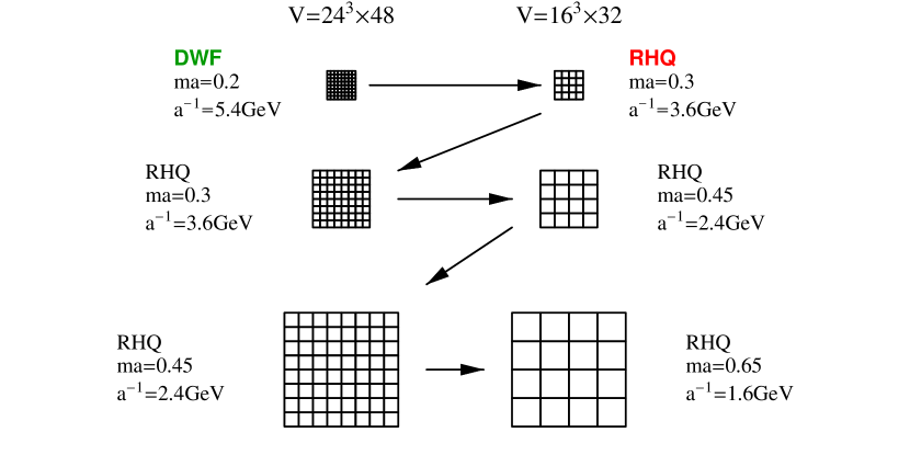
Figure 1: The sequence of lattice sizes and lattice spacings used to determine the coarse-lattice, heavy quark parameters through a step-scaling technique beginning with a comparison with an $O(a)$-improved light quark calculation. The matching between the top two lattice spacings is the calculation described in this paper.

We propose to determine the three coefficients $m_{0}$, $\zeta$ and $c_{P}\equiv c_{B}=c_{E}$ in the RHQ lattice action of Eq. 1 by carrying out a series of matching steps. We begin with a sufficiently fine lattice spacing that no heavy quark improvements are needed ($ma\ll 1$) and a conventional light-quark calculation will give accurate results. We then carry out a series of calculations using the RHQ lattice action of Eq. 1 on lattices with increasingly large lattice spacing and increasingly large physical volume. When we increase the lattice spacing at fixed physical volume, we perform calculations at both lattice spacings on identical physical volumes and require that the resulting finite-volume, heavy-heavy and heavy-light energy spectrum agree when these particles are at rest or have small spatial momenta. When we increase the lattice volume at fixed lattice spacing, we simply use the parameters, previously determined, in a calculation now on the larger volume. The first same-physical-volume matching of the energy spectrum is done between the heavy quark theory and a conventional fine-lattice calculation done with domain wall fermions. An example of this finite volume, step-scaling recursion is shown in Fig. 1.

Specifically, we will calculate the pseudo-scalar (PS), vector (V), scalar (S), and axial-vector (AV) meson masses in the heavy-heavy ($hh$) system and pseudo-scalar and vector masses for the heavy-light ($hl$) system. We will work with the following mass combinations:

• Spin-average: $m^{hh}_{\rm sa}=\frac{1}{4}\left(m^{hh}_{\rm PS}+3m^{hh}_{\rm V}\right)$, $m^{hl}_{\rm sa}=\frac{1}{4}\left(m^{hl}_{\rm PS}+3m^{hl}_{\rm V}\right)$

• Hyperfine splitting: $m^{hh}_{\rm hs}=m^{hh}_{\rm V}-m^{hh}_{\rm PS}$, $m^{hl}_{\rm hs}=m^{hl}_{\rm V}-m^{hl}_{\rm PS}$

• Spin-orbit average and splitting: $m^{hh}_{\rm soa}=\frac{1}{4}\left(m^{hh}_{\rm S}+3m^{hh}_{\rm AV}\right)$, $m^{hh}_{\rm sos}=m^{hh}_{\rm AV}-m^{hh}_{\rm S}$

• Mass ratio: $m_{1}/m_{2}$ where $E^{2}=m_{1}^{2}+\frac{m_{1}}{m_{2}}p^{2}$, with $m_{1}$ the rest mass and $m_{2}$ the kinetic mass.

By examining these seven quantities we should be able to determine the three parameters $m_{0}$, $\zeta$ and $c_{P}$ and also check the size of the scaling violations.

The first step in this program calculates these seven quantities using the domain wall fermion action on the fine, $24^{3}\times 64$ lattice with $1/a=5.4$ GeV (I). Next, these seven quantities are computed a second time using a coarse, $16^{3}\times 32$ lattice with $1/a=3.6$ GeV and, therefore, the same physical volume. This is calculation II. The three heavy-quark parameters entering this coarse-lattice calculation must be adjusted so that these seven quantities agree between calculations I and II. It is these calculations that are carried out in this paper using the parameters given in Table 2.

Third, we expand the volume of calculation II to $24^{3}\times 48$, while keeping all other parameters fixed. The results of this third, expanded volume calculation (III) can then be matched with a fourth calculation which has a lattice spacing larger by a factor of 3/2 (IV). The simulation parameters for this second matching step are given in Table 3. By repeating this pattern, we can extend the calculation to quenched lattices with the desired volume where serious, infinite-volume, charm physics may be studied.

In this paper, we demonstrate only the matching between calculations I and II. The leading heavy quark discretization error in calculation I is $(ma)^{2}\approx 4\%$, making it the dominant systematic error on the fine lattice result. Of course, this error can be reduced in future calculations by choosing a fine lattice that has an even smaller lattice spacing and correspondingly smaller physical volume. Without improvement beyond the usual Sheikholeslami and Wohlert term, the leading heavy quark discretization error on the coarse lattice is expected to be $(ma)^{2}\approx 10\%$. However, once we introduce the improved lattice action of Eq. 1 and properly tune the coefficients, we should be able to reduce the error to $(a|{\mathchoice{\!\stackrel{{\scriptstyle{}_{{}_{\>\scriptstyle\rightarrow}}}}{{\displaystyle p}}\!}{\!\stackrel{{\scriptstyle{}_{{}_{\>\scriptstyle\rightarrow}}}}{{\textstyle p}}\!}{\!\stackrel{{\scriptstyle{}_{{}_{\>\scriptscriptstyle\rightarrow}}}}{{\scriptstyle p}}\!}{\!\stackrel{{\scriptstyle{}_{{}_{\>\scriptscriptstyle\rightarrow}}}}{{\scriptscriptstyle p}}\!}}|)^{2}\approx 1\%$.

As will be demonstrated in the remainder of this paper, this proposed step-scaling method works well and offers a feasible approach to heavy quark calculations with accurately controlled finite lattice spacing errors. However, unless we can move beyond the quenched approximation used here, this method will be of only limited utility. Using this method for full QCD will, of course, be more computationally demanding because each of the two sets of lattice configurations generated for this matching process must be obtained from a full, dynamical simulation including the quark determinant. However, such an approach could become prohibitively expensive if the value of the light dynamical quark masses, $m_{\rm light}a$, must to decrease toward zero with decreasing $a$.

Fortunately, such small dynamical quark masses are not required in this step-scaling approach. The combination of the usual gauge and light-quark action together with the effective lattice action of Eq. 1 defines a complete physical theory, including the properties of heavy quarks, that is unambiguously specified at short distances $\lambda$ with $a\ll\lambda\ll 1/m_{\rm light}$. Recall that in the continuum such a local field theory is typically defined in a mass- and volume-independent fashion. Short-distance renormalization conditions are imposed to fix the theory in a manner that is insensitive to quark masses and space-time volumes. Similarly our fine-lattice theory, viewed as a function of the bare input lattice parameters also defines such a mass- and volume-independent theory.

Given sufficient computer power, the implications of this theory could be worked out on arbitrarily large spatial volumes and for arbitrarily small masses. The results would be well-defined functions of the bare input parameters which would require no adjustment as the quark mass and spatial volume were varied. The lattice spacing could be determined in physical units by comparing to $\Lambda_{\rm QCD}$ as determined from a vertex function at short distances with the light quark masses having a negligible effect.

Replacing the standard light quark action appropriate for our finest lattice with the improved lattice action of Eq. 1 does not change this situation. The parameters in the heavy quark action could be evaluated or renormalized by examining Green’s functions evaluated at non-exceptional momenta without infra-red or light-quark mass sensitivity Lin (2004, 2005a). We would still be working with a short-distance-defined field theory that will give meaningful predictions as a function of lattice volume and light quark mass. Thus, when comparing two such effective theories defined at two different lattice spacings we are free to use any lattice size $L$ and dynamical quark mass $m_{\rm light}$ we find convenient provided $L\gg a$ and $m_{\rm light}\ll 1/a$. In fact, if $m_{\rm light}$ is sufficiently small that it does not effect the finite-volume heavy-quark spectrum being compared, we need not even use the same quark mass in the two calculations being compared! Of course, this is likely a quark mass that is expensively small and a better strategy is to work with sufficiently small spatial volume and sufficiently heavy dynamical quark mass that they do effect the quantities being matched and must be given equivalent physical values in each of the calculations being compared.

We conclude that employing the procedure developed here in full QCD, while difficult, is practical and well within the reach of present computer resources. Just as our step-scaled lattice spacing decreases and we move to increasingly smaller spatial volumes, we should also move to increasingly heavier quark masses. In both cases finite volume and finite dynamical quark mass effects are distorting the spectrum being compared, but these distortions are entirely physical and must be accurately described by the effective actions being compared.

III Simulations

We performed this calculation on a 512-node partition of the QCDOC machine located at Columbia University. We used the Wilson gauge action since for this case the relation between lattice coupling and lattice spacing has been thoroughly studied Guagnelli et al. (1998); Necco and Sommer (2002).

The gauge configurations were generated using the heatbath method of Creutz Creutz (1980), adapted for $SU(3)$ using the two-subgroup technique of Cabibbo and Marinari Cabibbo and Marinari (1982). The first 20,000 sweeps were discarded for thermalization and configurations thereafter were saved and analyzed every 10,000 sweeps. We examined the auto-correlation between configurations for both the standard 4-link plaquette and the hadron propagators evaluated at a time separation of 12 lattice units. Here we use the standard autocorrelation function $\rho(t)$ as

$$\rho(t)=\frac{1}{N_{tot}-t}\sum_{j}^{N_{tot}-t}\left(O(j)-\overline{O}\right)\left(O(t+j)-\overline{O}\right)$$ (5)

and identify the autocorrelation time as the size of the region near $t=0$ in which $\rho(t)\neq 0$.

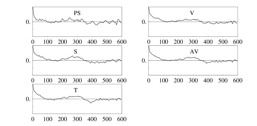
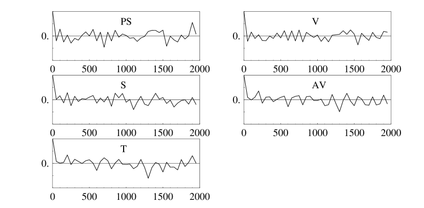
Figure 2: The auto-correlation function for five different heavy-heavy meson propagators evaluated at a source-sink separation of twelve lattice units with $\beta=6.638$ and a $24^{3}\times 48$ space-time volume. In the top graph the propagators were calculated on every 5th configuration while in the bottom graph the propagator measurements were separated by 50 sweeps. This suggests that our separation of 10,000 sweeps between measurements ensures that they will be uncorrelated.

For the case of the plaquette (which was calculated every sweep) we found an auto-correlation time of approximately 3 sweeps. We studied the propagator correlations using two $24^{3}\times 32$, $\beta=6.638$ test calculations: in the first, the propagators were computed on 120 configurations, separated by 5 sweeps and in the second on 40 configurations separated by 50 sweeps. The resulting correlations functions for five different hadron propagators evaluated at a temporal source-sink separation of twelve lattice units are shown in Fig. 2. Auto-correlation on the scale of 100 sweeps can be seen in the data sampled every five sweeps. Essentially no autocorrelation can be seen for the propagators sampled every fifty sweeps. Since we used a total of 100 such lattice configurations, separated by 10,000 sweeps, for all of the quantities discussed in this paper, we will assume that quantities calculated on different configurations are statistically independent.

III.1 Lattice scale

Four different quantities with a meaningful physical scale enter each of the two lattice calculations that must be matched at a given stage in our step-scaling procedure. Most familiar is the distance scale determined by the static quark potential or the chiral limit of the light hadron spectrum. This is an important physical scale that will influence even small-volume, heavy quark results. As is conventional, we will refer to this quantity as the “lattice spacing”. We will find it convenient to determine this from direct calculation of the static quark potential. The other three scales are the lattice volume, and the masses of the light and heavy quarks. (In our discussion of heavy-light systems we will ignore the strange quark and work with degenerate up and down quarks.)

Of course, the lattice spacing, expressed in physical units, is also important since it gives us a direct idea of the size of the discretization errors which we are trying to control. For this purpose we don’t need great precision (something that cannot be achieved in a quenched calculation under any circumstances). We will determine the lattice spacing in physical units from the static quark potential evaluated at an intermediate distance to yield the Sommer scale Guagnelli et al. (1998) which is then determined from a phenomenological, static quark potential model. While the later is not precisely defined, this method has the advantage that it uses only pure gauge theory without any fermion action being involved. We could get a physical value for the lattice scale from the pion decay constant $f_{\pi}$ or the rho meson mass but these are more difficult to calculate and may be more sensitive to finite volume and other systematic errors.

Our strategy for choosing the parameters to be used on the fine lattice and then finding physically equivalent parameters to be used on the coarser lattice proceeds as follows. We first decide on a target ratio of lattice scales determined by the ratio of lattice volumes that we intend to use. In the present case a ratio of $3/2$ is implied by our choice of $24^{3}$ and $16^{3}$ lattice volumes. Second, we choose the bare lattice coupling on the fine lattice to insure that the fine lattice spacing is sufficiently small (here chosen to be $1/a=5.4$ GeV). The stronger coupling must then give a lattice spacing larger by a factor of 3/2 than the fine value or $1/a=3.6$ GeV. While for a dynamical QCD calculation, this would require considerable numerical exploration, for a quenched calculation with the Wilson gauge action, we can simply refer to extensive earlier work.

Next we choose the light quark mass to be used on the fine lattice as sufficiently light that the heavy-light mesons being studied will be involve a different momentum scale than do the heavy-heavy mesons but not so light as to unreasonably increase the computational cost. For the calculations reported here we used the domain wall formalism for the light quarks and chose the mass $m_{f}a=0.02$, one-tenth of the 0.2 heavy quark mass. The light quark mass to be used on the coarse lattice is determined by requiring that the light-light pseudo-scalar meson have a mass 3/2 times larger than that found on the fine lattice when measured in lattice units.

Finally the heavy quark mass on the fine lattice is estimated to correspond to the bare charm quark mass. While in the present calculation we have used the single value $m_{f}a=0.2$, a complete calculation will likely require one or two more masses so that a final interpolation/extrapolation can be done to make the physical charmed hadron mass agree with experiment. The heavy quark mass on the coarse lattice is one of the three heavy-quark parameters whose determination is discussed in the next section.

Let us now discuss the choice of lattice scale in more detail. The static potential is expected to have the following form

$$V(R)=C-\frac{\alpha}{R}+\sigma R$$ (6)

where R is the separation between the static quarks. The scale implied by the heavy quark potential is often specified using the Sommer parameter $r_{0}$ which is defined by the condition

$$-R^{2}\frac{\partial V(R)}{\partial R}|_{R=r_{0}}=1.65.$$ (7)

This is appropriate on standard size lattices for bare couplings in the range $\beta=6/g^{2}\leq 6.57$. For weaker couplings, $\beta>6.57$ one uses a second, smaller distance scale, $r_{c}$ defined by

$$R^{2}F(R)|_{R=r_{c}}=0.65$$ (8)

where $\frac{r_{c}}{r_{0}}=0.5133(24)$ Necco and Sommer (2002). While it may be problematic in a quenched calculation, we can attempt to determine $r_{0}$ from a phenomenological potential model, which gives $r_{0}^{-1}=0.395$ GeV.

Reference Necco and Sommer (2002) gives predictions for the resulting lattice spacing when the coupling $\beta$ of Wilson gauge action is in the range $5.7~{}\leq\beta~{}\leq 6.92$:

$$\ln(a/r_{0})=-1.6804-1.7339(\beta-6)+0.7849(\beta-6)^{2}-0.4428(\beta-6)^{3}.$$ (9)

With the help of Eq. 9, we can locate the $\beta$ values needed to achieve the desired cutoff scales and fine tune it later as necessary. As our final choices, we have $\beta=6.638$ for the $a^{-1}=5.4$ GeV lattice and $\beta=6.351$ for the $a^{-1}=3.6$ GeV one.

Since the comparison of lattice scales between our two simulations is fundamental to this matching program, we have carried out additional calculations to make sure that the lattice spacing is correctly selected. This requires a direct calculation of the static quark potential on our lattice configurations.

Recall that the static quark potential can be extracted from the ratio of Wilson loops:

$$V({\mathchoice{\!\stackrel{{\scriptstyle{}_{{}_{\>\scriptstyle\rightarrow}}}}{{\displaystyle r}}\!}{\!\stackrel{{\scriptstyle{}_{{}_{\>\scriptstyle\rightarrow}}}}{{\textstyle r}}\!}{\!\stackrel{{\scriptstyle{}_{{}_{\>\scriptscriptstyle\rightarrow}}}}{{\scriptstyle r}}\!}{\!\stackrel{{\scriptstyle{}_{{}_{\>\scriptscriptstyle\rightarrow}}}}{{\scriptscriptstyle r}}\!}})=\log\left[\frac{\langle W({\mathchoice{\!\stackrel{{\scriptstyle{}_{{}_{\>\scriptstyle\rightarrow}}}}{{\displaystyle r}}\!}{\!\stackrel{{\scriptstyle{}_{{}_{\>\scriptstyle\rightarrow}}}}{{\textstyle r}}\!}{\!\stackrel{{\scriptstyle{}_{{}_{\>\scriptscriptstyle\rightarrow}}}}{{\scriptstyle r}}\!}{\!\stackrel{{\scriptstyle{}_{{}_{\>\scriptscriptstyle\rightarrow}}}}{{\scriptscriptstyle r}}\!}},t)\rangle}{\langle W({\mathchoice{\!\stackrel{{\scriptstyle{}_{{}_{\>\scriptstyle\rightarrow}}}}{{\displaystyle r}}\!}{\!\stackrel{{\scriptstyle{}_{{}_{\>\scriptstyle\rightarrow}}}}{{\textstyle r}}\!}{\!\stackrel{{\scriptstyle{}_{{}_{\>\scriptscriptstyle\rightarrow}}}}{{\scriptstyle r}}\!}{\!\stackrel{{\scriptstyle{}_{{}_{\>\scriptscriptstyle\rightarrow}}}}{{\scriptscriptstyle r}}\!}},t+1)\rangle}\right]$$ (10)

where $\langle\ldots\rangle$ denotes an average over gauge configurations. In order to improve the signal and to extract the potential $V(r)$ from smaller time separations, we smear the gauge links in the spatial directions according to Ref. Albanese et al. (1987)

$$U_{k}(n)\rightarrow P_{{\rm SU}(3)}\left[U_{k}(n)+c_{\rm smear}\sum_{\rm l\neq k}U_{l}(n)U_{k}(n+\hat{\rm{l}})U_{-l}(n+\hat{l}+\hat{k})\right]$$ (11)

where $k$ and $l$ each indicate a spatial direction, $P_{{\rm SU}(3)}$ is an operator that projects a link back to an ${\rm SU}(3)$ special unitary matrix, $c_{\rm smear}$ is the smearing coefficient (set to 0.5 in our case) and the smearing procedure is performed $n_{\rm smear}$ times. More details regarding the algorithm can be found in Ref. Hashimoto and Izubuchi (2005); Aoki et al. (2004b). In our calculation we found good results for $n_{\rm smear}=180$ for the fine lattice and $n_{\rm smear}=60$ for the coarse one.

While we did determine the two scale standards $r_{0}$ and $r_{c}$ individually for both of our lattice spacings, our lattice volumes are somewhat small to permit a comparison with infinite volume results. We therefore also determined the ratio of lattice spacings without using the Sommer scale by directly comparing the potentials computed on our two sets of lattice configurations using the relation

$$V_{1}(n)=V_{2}(n/\lambda)/\lambda+C^{\prime}$$

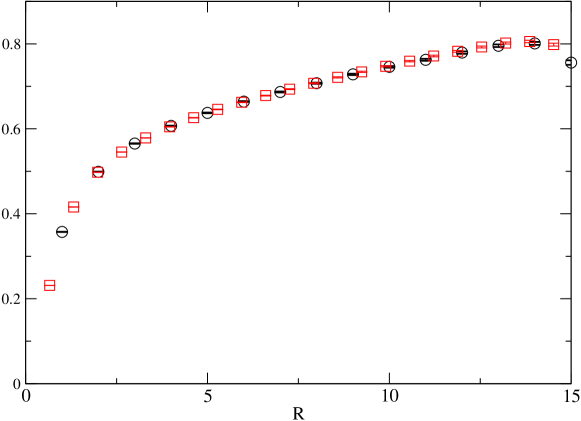
Figure 3: The static quark potential calculated on both the coarse and fine lattices. The static quark potential values computed on the $\beta=6.351$ lattice are shown as circles. The squares mark the static quark potential from the $\beta=6.638$ lattice scaled by the fitted ratio of lattice spacings $\lambda=1.51$ and shifted by a constant. The agreement between these two different sets of points gives good evidence that the ratio of lattice spacings between these two $\beta$ values is the desired 3/2.

where $\lambda={a_{2}}/{a_{1}}$ is the ratio of the two lattice spacings. We first fit the static potential on the fine lattice to the form given in Eq. 6, determining the parameters $C$, $\alpha$ and $\sigma$. Next we scaled the resulting fitted function according to Eq. III.1 and adjusted the parameters $\lambda$ and $C^{\prime}$ in that equation to obtain the best fit to the static potential measured on the coarse lattice. Figure 3 shows a comparison of the potential determined from $\beta=6.351$ configurations and a scaled and shifted version of the $\beta=6.638$ potential. The agreement is excellent and this procedure gives an independent value for the lattice spacing ratio of $1.51(2)$, which agrees with what we wanted.

III.2 Domain-Wall Fermions

We will now briefly describe the domain wall fermion calculations that were used for the heavy quark on the finest lattice and the light quarks on both lattices. The domain wall Dirac operator can be written as

$$D_{x,s;x^{\prime},s^{\prime}}=\delta_{s,s^{\prime}}D^{\parallel}_{x,x^{\prime}}+\delta_{x,x^{\prime}}D^{\bot}_{s,s^{\prime}}$$

$$D^{\parallel}_{x,x^{\prime}} = {1\over 2}\sum_{\mu=1}^{4}\left[(1-\gamma_{\mu})U_{x,\mu}\delta_{x+\hat{\mu},x^{\prime}}+(1+\gamma_{\mu})U^{\dagger}_{x^{\prime},\mu}\delta_{x-\hat{\mu},x^{\prime}}\right]+(M_{5}-4)\delta_{x,x^{\prime}}$$ (12)

$$D^{\bot}_{s,s^{\prime}} = {1\over 2}\Big{[}(1-\gamma_{5})\delta_{s+1,s^{\prime}}+(1+\gamma_{5})\delta_{s-1,s^{\prime}}-2\delta_{s,s^{\prime}}\Big{]}$$ (13)

$$- {m_{f}\over 2}\Big{[}(1-\gamma_{5})\delta_{s,L_{s}-1}\delta_{0,s^{\prime}}+(1+\gamma_{5})\delta_{s,0}\delta_{L_{s}-1,s^{\prime}}\Big{]}.$$

where the fifth-dimension indices $s$ and $s^{\prime}$ lie in the range $0\leq s,s^{\prime}\leq L_{s}-1$, $M_{5}$ is the five-dimensional mass and $m_{f}$ directly couples the two walls at $s=0$ and $s=L_{s}-1$. It is related to the physical mass of the four-dimensional fermions.

The $M_{5}$ parameter is optimized by the choice of $M_{5}\approx 1-m_{\rm crit}$, where $m_{\rm crit}$ is the critical value of the mass for the 4-dimensional Wilson fermion action. This quantity has been calculated perturbatively up to one-loop level for the Wilson gauge action and either the WilsonFollana and Panagopoulos (2001) or SWPanagopoulos and Proestos (2002) fermion actions. In the quenched approximation, for Wilson fermions and with our choices of gauge coupling, we find $m_{\rm crit}=-0.495$ at $\beta=6.638$, and $m_{\rm crit}=-0.522$ at $\beta=6.351$. Therefore, we use $M_{5}=1.5$ in the DWF action for both our $\beta$ values.

The DWF action is $O(a)$ off-shell improved due to the preservation of chiral symmetry, and no further improvement in the action or quark fields is performed. The chiral symmetry breaking can be measured from the residual mass, which can be computed from the ratio

$$am_{\rm res}=\frac{\sum_{x}\langle J_{5q}^{a}({\mathchoice{\!\stackrel{{\scriptstyle{}_{{}_{\>\scriptstyle\rightarrow}}}}{{\displaystyle x}}\!}{\!\stackrel{{\scriptstyle{}_{{}_{\>\scriptstyle\rightarrow}}}}{{\textstyle x}}\!}{\!\stackrel{{\scriptstyle{}_{{}_{\>\scriptscriptstyle\rightarrow}}}}{{\scriptstyle x}}\!}{\!\stackrel{{\scriptstyle{}_{{}_{\>\scriptscriptstyle\rightarrow}}}}{{\scriptscriptstyle x}}\!}},t)\pi(0)\rangle}{\sum_{x}\langle J_{5}^{a}({\mathchoice{\!\stackrel{{\scriptstyle{}_{{}_{\>\scriptstyle\rightarrow}}}}{{\displaystyle x}}\!}{\!\stackrel{{\scriptstyle{}_{{}_{\>\scriptstyle\rightarrow}}}}{{\textstyle x}}\!}{\!\stackrel{{\scriptstyle{}_{{}_{\>\scriptscriptstyle\rightarrow}}}}{{\scriptstyle x}}\!}{\!\stackrel{{\scriptstyle{}_{{}_{\>\scriptscriptstyle\rightarrow}}}}{{\scriptscriptstyle x}}\!}},t)\pi(0)\rangle},$$ (14)

provided $t\gg a$. Here $J_{5q}$ is a pseudoscalar density located at the midpoint of the fifth dimension. The residual mass has been thoroughly studied, for example, in Ref.Aoki et al. (2004c) for various values of $\beta$, $L_{s}$ and $M_{5}$. Those results suggest that the $m_{\rm res}$ values for each of our lattice configurations are much smaller than the 0.00124 value determined at $\beta=6.0$ with lattice volume $16^{3}\times 32\times 16$ and $M_{5}=1.8$. This indicates that chiral symmetry breaking is small and ignoring the contribution of $m_{\rm res}$ in the heavy quark sector will have an effect smaller than 0.5%.

However, there is a limitation to using large values of $m_{f}$ with DWF. Recall that there are two types of eigenvectors of the hermitian DWF Dirac operator: propagating and decaying statesChrist and Liu (2004); Liu (2003). The former, unphysical states have non-zero $5^{th}$-dimension momenta and large Dirac eigenvalues around $1/a$. The “decaying” states are bound to the walls of the $5^{\rm th}$ dimension and are the physical states corresponding to the four-dimensional Dirac eigenstates in the continuum limit. The gap between these two types of states is controlled by the domain-wall height $M_{5}$. However, as $m_{f}$ increases, the eigenvalues of the physical states increase while those of the propagating states do not. Thus, we must be careful to avoid the situation in which the states with the smallest eigenvalues are dominated by these unphysical states. Therefore, a careful check on the lowest eigenvalues for the target $m_{f}$ being used to simulate the heavy quarks on the fine lattice is needed. Figure 4 shows the 5-dimensional eigenfunction, averaged over 4-dimensional space, $\sum_{x}|\Psi_{x,s}|^{2}$ as a function of the $5^{\rm th}$-dimensional coordinate $s$ for the lowest nineteen eigenvalues with various $m_{f}$: 0.22, 0.27, 0.37, 0.47. As can be seen in the figure, these first nineteen eigenfunctions appear to be physical states bound to the 4-dimensional wall for the first three mass values. However, $m_{f}=0.047$ is sufficiently large that propagation into the 5-dimension can be clearly seen. We conclude that our $m_{f}=0.2$ for the heavy quark is safe, well below the region where such unphysical states arise.

III.3 Spectrum Measurements

In order to get good signals for the heavy quark states of interest for relatively small time separations, a smeared wavefunction source is used for the heavy quark (but not the light quark). Here, we adopt the Coulomb gauge-fixed hydrogen ground-state wavefunction:

$$\Psi_{gnd}(r) = e^{-r/r_{0}}$$ (15)

as the source of the heavy fermion(s) and use a point source for the light fermion (if any). At the sink the two propagators are evaluated at the same point and the resulting gauge invariant combination summed over a 3-dimensional plane at fixed time, with a possible momentum projection factor. An optimized radius, $r_{0}$, was chosen in the fashion suggested in Ref. Boyle (2002). Table 4 lists all the local meson operators used in our calculation.

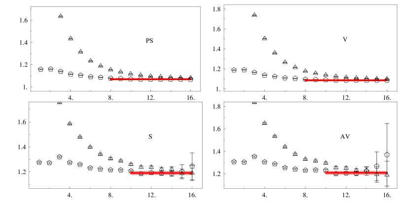
Figure 5: A comparison of effective mass plateaus between point and smeared sources in the heavy-heavy sector. Triangles denote the point-point source, and pentagons denote the point-smeared heavy meson correlators. Clearly, the plateaus have been improved by the smearing. However, a double-cosh fit to the two distinct wavefunction sources might help us determine the ground state energy even more accurately.

Figure 5 shows how the plateau in the effective mass plot improves between a point and smeared source. The smeared-source meson plateaus are much better those of the local source, even for the scalar and axial-vector mesons.

To constrain the space-time asymmetry parameter $\zeta$, we also computed the pseudo-scalar meson energy in the heavy-heavy sector for the three lowest on-axis momenta: $\frac{2\pi}{L}(0,0,0)$, $\frac{2\pi}{L}(0,0,1)$, and $\frac{2\pi}{L}(0,1,1)$, where $L$ is the spatial lattice size. The dispersion relation may be expanded in momentum as

$$E(p) = m_{1}+\frac{p^{2}}{2m_{2}}+O(p^{4}).$$ (16)

As we will see, requiring the ratio of static to kinetic mass, $m_{2}/m_{1}=1$ is useful for determining the coefficient $\zeta$.

III.4 Parameters

Table 5 lists the fixed parameters used throughout this matching stage for the fine and coarse lattices. The heavy quark mass was set to approximate that of the charm mass and the light quark mass was chosen ten times smaller. The lattice spacing ratio between these two lattices is 1.5. The domain wall fermion parameters used on the fine lattice have been carefully studied and we find no unphysical states in the chosen mass range as discussed in previous section. Table 6 shows the hadron mass spectrum computed on the fine lattice. As can be seen, $m_{1}/m_{2}=1.02(2)$ is consistent with 1, indicating that heavy quark discretization effects using domain wall fermions are small. One expects that the light quark mass on the coarse lattice should be 0.03 and the data for the light-light spectrum with this choice of light quark mass is listed in Table 7. As one can see from Table 7, the light-light meson spectra on the coarse and fine lattices agree when compared in the same units, indicating that the light quark mass is well tuned on the coarse lattice.

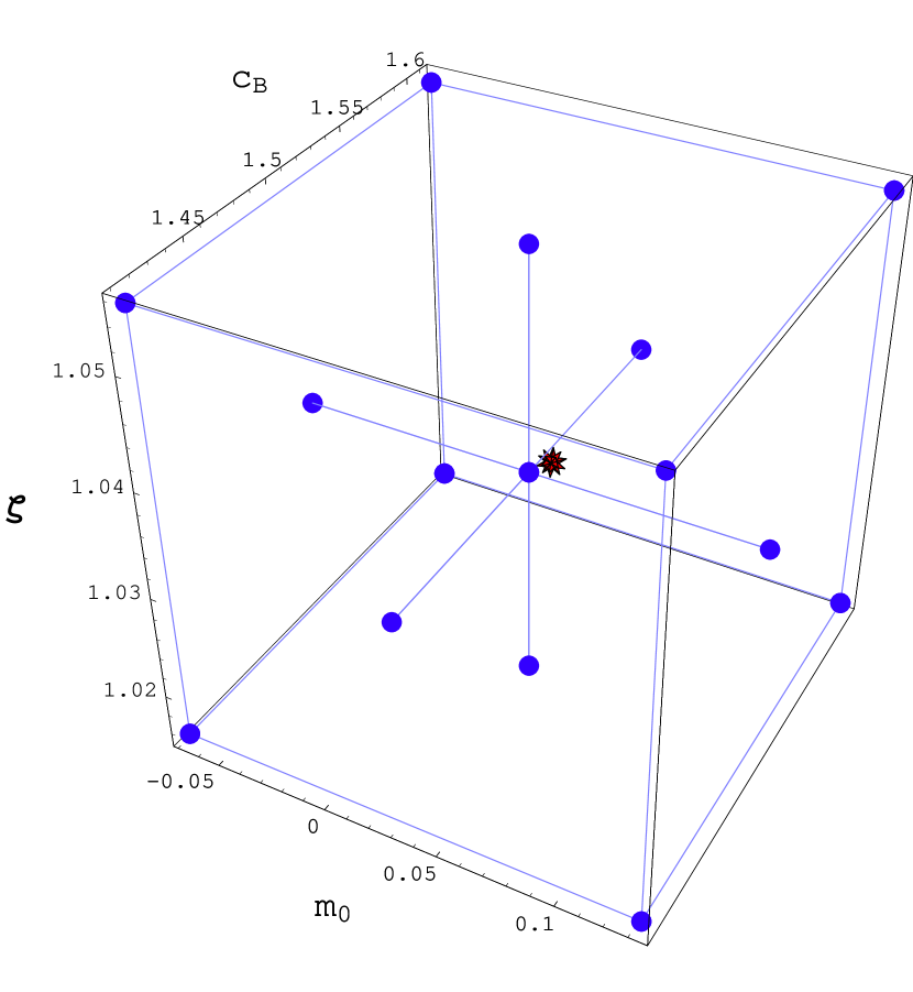
Figure 6: The distribution in the 3-parameter space ($m_{0}$, $c_{B}$, $\zeta$) of the 24-set “Cartesian” data. The center circular point is set #14, and the points around it are sets#43-66. The starred point represents the final matching coefficients determined in Sec. IV.2.

A complete list of the parameter sets used for the RHQ action on the coarse lattice is given in Table 8. The first 42 sets of data were initial trials chosen to give good coverage in parameter space. In order to perform a more systematic analysis, described in Sec. IV, we also collected a “Cartesian” set (sets #43-#66) chosen close to the desired fine lattice measurements. These 24 data sets are centered around set #14. The range of each parameter in this Cartesian data set was selected so that within that range the estimated difference between a linear and quadratic fit would be less than 5% as expected from an examination of the first 42 parameter sets. This yields a region that is close to reproducing the target fine data and in which a linear approximation should be good: $m_{0}=0.0328\pm 0.1$, $c_{B}=1.511\pm 0.1$, $c_{E}=1.538\pm 0.3$ and $\zeta=1.036\pm 0.02$, which is shown in Figure 6.

The 24-set “Cartesian” data will allow us to calculate the first and second derivatives directly from the measurements. Note that we have more measurements than we actually need. This provides additional checks on our method and the validity of the scaling of physical quantities between the coarse and fine lattices. We expect that the total number of data sets that we will use for next step of matching will be dramatically reduced.

Using the methods described in Sec. III.3, we have measured the pseudoscalar (PS), vector (V), scalar (S) and axial-vector (AV) mesons in the heavy-heavy system, and PS and V in the heavy-light system. We use combinations of the masses to try to simplify their dependence on the coefficients of the RHQ action. For the heavy-light system, we use the spin-average and hyperfine splitting; for the heavy-heavy system, we use these and also include the spin-orbit average, spin-orbit splitting and the ratio of $m_{1}/m_{2}$. The resulting values for these quantities for each of the 66 data sets are given in Table 9.

IV Analysis and Results

The final step in this matching procedure is to determine the parameters in the heavy quark action of Eq. 1, $\{m_{0},c_{B},c_{E},\zeta\}$, that will yield the seven quantities measured on the coarse lattice which agree with those determined on the fine lattice. Of course, this might be done by “trial and error” and, as can be seen by scaling the numbers in Table 9, data set #14 comes very close to such a result. However, to fully understand this step scaling method (for example to properly propagate errors) it is important to learn in detail how the measured spectra depend on these input parameters.

As a starting point, we will attempt to use a subset of our parameter space chosen so that the resulting coarse lattice hadron masses are well fit by a simple linear dependence on the heavy quark parameters:

$$Y^{n}=A+J\!\cdot\!X^{n},$$ (17)

where $n$ labels the parameter set while $X$ and $Y$ are 4-dimensional and 7-dimensional column vectors made up of the four input heavy-action parameters and the seven computed masses or mass ratios, respectively:

$$X=\left(\begin{array}[]{c}m_{0}\\ c_{B}\\ c_{E}\\ \zeta\end{array}\right)\quad Y=\left(\begin{array}[]{c}m^{hh}_{sa}\\ m^{hh}_{hs}\\ m^{hl}_{sa}\\ m^{hl}_{hs}\\ m^{hh}_{soa}\\ m^{hh}_{sos}\\ m_{1}/m_{2}\end{array}\right).$$ (18)

The quantities $A$ and $J$ are a 7-dimensional column vector and a $7\times 4$ matrix which represent the constant and linear terms in our linear approximation. (In most of the discussion to follow we will work with all seven measured quantities. However, if this number is decreased, the vectors $Y$, $A$ and the matrix $J$ will shrink appropriately.)

Given a specific group of $N$ of our data sets, $X^{n_{i}}|_{1\leq i\leq N}$, we can determine the quantities $A$ and $J$ by minimizing an appropriate $\chi^{2}$ for such a linear fit:

$$\chi_{\cal C}^{2}=\sum_{i=1}^{N}(A+J\!\cdot\!X^{n_{i}}-Y^{n_{i}})^{T}\!\cdot\!W_{\cal C}^{-1}\!\cdot\!(A+J\!\cdot\!X^{n_{i}}-Y^{n_{i}}).$$ (19)

Here $W$ is a $7\times 7$ matrix representing a choice of correlation matrix. In the results that follow we will use

$$(W_{\cal C})_{d,d^{\prime}}=\sum_{i=1}^{N}\langle\Bigl{(}Y^{n_{i}}_{d}-\overline{Y}^{n_{i}}_{d}\Bigr{)}\Bigl{(}Y^{n_{i}}_{d^{\prime}}-\overline{Y}^{n_{i}}_{d^{\prime}}\Bigr{)}\rangle$$ (20)

where $\langle...\rangle$ represents an average over the 100 jackknife blocks obtained by omitting one of the 100 measurements with $Y^{n_{i}}_{d}$ the result for that jackknife block and $\overline{Y}^{n_{i}}_{d}$ the corresponding average. Replacing $W_{\cal C}$ by the simpler, uncorrelated error matrix $(W_{\cal C}^{\prime})_{d,d^{\prime}}=\sum_{i=1}^{N}\delta_{d,d^{\prime}}\sigma^{n_{i}}_{d}$ had little effect on the final results where $\sigma^{i}_{d}$ is the usual squared error on the measured quantity $Y^{i}_{d}$. Determining the $A$ and $J$ which minimize $\chi_{\cal C}^{2}$ is straight-forward because this is a quadratic function of these 35 numbers and the minimum can be obtained by solving 35 linear equations. Typically these 35 equations are quite regular, with a stable solution even if only a relative few of our data sets are used.

The use of linearity to determine the desired matching heavy quark parameters is reasonable if we are working in a region that is close to the right choice for those parameters. Once we have determined the matrix $J$ and vector $A$, we can solve for the coefficients $X_{\cal C}$ that will yield meson masses equal to those found on the fine lattice, $Y_{\cal F}$. Here we add the subscripts $\cal C$ and $\cal F$ to indicate our estimates for the physical coarse-lattice parameters ($X_{\cal C}$) and the coarse-lattice masses ($Y_{\cal F}$), scaled from those calculated using the fine lattice.

Again we minimize a quantity $\chi_{\cal F}^{2}$, similar to that given in Eq. 19. However, the fine-lattice correlation matrix, $W_{\cal F}$, which appears in the equivalent version of Eq. 19 is defined through a modified version of Eq. 20. Specifically, the fine-data analogue of Eq. 20 is used for all but the seventh row and seventh column, which correspond to the quantity $m_{1}/m_{2}$. Since this must be unity in a relativistic calculation (and is one within errors for our DWF results), we set $(Y_{\cal F})_{6}=1$ and the corresponding elements of the correlation $(W_{\cal C})_{d\neq 6,6}=(W_{\cal C})_{6,d\neq 6}=0$ for $0\leq d\leq 6$. In order that the resulting correlation matrix be invertible, we arbitrarily set $(W_{\cal C})_{6,6}=10^{-8}$. This has the effect of constraining the coarse-lattice value of $m_{1}/m_{2}=1$. The resulting minimum is again determine by solving a set of linear equations. That solution can be written explicitly as:

$$X_{\cal C} = \left(J^{T}\!\cdot\!W^{-1}_{\cal F}\!\cdot\!J\right)^{-1}\!\cdot\!J^{T}\!\cdot\!W_{\cal F}\!\cdot\!\left(Y_{\cal F}-A\right).$$ (21)

Finally, to determine the error on the resulting heavy quark parameters $X_{\cal C}$ we add in quadrature two different sources of error. To compute the first, we use the average value of the masses $Y_{\cal F}$, deduced from the fine-lattice calculation, which together with jackknifed results for $J$ and $A$ gives us the error on $X_{\cal C}$ coming from the statistical fluctuations in the coarse lattice data. We then estimate the statistical error coming from the fine lattice calculation by using the average values for $J$ and $A$ in Eq. 21 and the jackknifed values of $Y_{\cal F}$ to determine the resulting fluctuations in the resulting heavy quark parameters, $X_{\cal C}$ caused by the statistical errors in the determination of $Y_{\cal F}$.

IV.1 Four-Parameter Action

As is suggested by the large number of data sets listed in Table 8, we had greater difficulty than expected in determining the four parameters $m_{0}$, $c_{B}$, $c_{E}$ and $\zeta$. Typically, reasonable choices of a subset of the parameter sets from the initial group of 42 parameter sets listed in Table 8 gave similar values for the final heavy quark parameters. However, the derivative matrix was typically quite singular and the resulting parameters, especially $c_{E}$, not well determined. In an attempt to make this process more deterministic, we collected the 24 Cartesian data sets from which we could determine the matrix of derivatives $J$ from simple differences. The result for $J$ agreed very well with that typically determined from the fitting procedure describe earlier to the less regular parameter choices in our first 42 data sets. We conclude that this linear description of our coarse lattice data is a good approximation. For simplicity, we present only the results from this final determination of $J$ and $A$ from the Cartesian data.

Specifically, the twenty four parameter choices within our Cartesian data set (#43-#66) use parameters of the form

$$X^{n}_{i}=\overline{X}_{i}+\sigma(n)_{i}\Delta_{i}.$$ (22)

Here the quantity $\{\sigma(n)_{i}\}_{0\leq i\leq 3}$ determines the first sixteen parameter choices, where $\sigma(n)_{i}=(-1)^{{\rm int}(n/2^{i})}$, the expression $\mbox{int}(x)$ represents the integer part of the number $x$ and the index $n$ varies between 0 and 15. The four parameter increments $\Delta_{0}=0.1$, $\Delta_{1}=0.1$, $\Delta_{2}=0.3$ and $\Delta_{3}=0.02$ were listed earlier and are displayed in Figure 6. The remaining eight data sets use the values $\sigma(16+n)_{i}=(-1)^{n}\delta_{{\rm int}(n/2),i}$ for $n=0,1\ldots 7$. The quantities $A$ and $J$ can be directly determined using the following expressions:

$$A_{d} = \frac{1}{24}\sum_{n=0}^{23}Y^{n}_{d}$$ (23)

$$J_{d,i} = \frac{1}{9}\sum_{n=0}^{23}\sigma(n)_{i}\frac{Y^{n}_{d}}{2\Delta_{i}}.$$ (24)

We can then substitute the resulting values of $A$ and $J$ into the linear relation of Eq. 17 and test this linear description of our coarse-lattice results for the 24 Cartesian data sets. The simplest test of linearity should be $\chi_{\cal C}^{2}$ of Eq. 19. However, for our 24 sets of seven quantities, the resulting $\chi_{\cal C}^{2}/(7\cdot 24)$ is $\approx 15$ suggesting this linear description is poor. This large value of $\chi_{\cal C}^{2}$ comes from the linear prediction of the heavy-heavy spin average masses. If these are dropped from the calculation of $\chi_{\cal C}^{2}$, we obtain $\chi_{\cal C}^{2}/(6\cdot 24)=1.7$, a much more acceptable value. Looking more closely, we find the linear prediction for the heavy-heavy spin average masses agrees with the calculated value with a fractional discrepancy of 1-2% for the 24 data sets. This is certainly a reasonable accuracy given the systematic errors in determining these masses from our lattice calculation. However, since the statistical error on these quantities, which is used in our definition of $\chi_{\cal C}^{2}$, is of the order of 0.1-0.2% we should expect these large $\chi_{\cal C}^{2}$ values. Thus, we conclude that the linear description of the coarse lattice results is satisfactory.

Using these results for $J$ and $A$, Eq. 21 and the procedure outlined in the previous section to determine the error we can go on to find the coarse lattice parameters which describe the fine lattice results:

$$X_{\cal C}^{T}=\{m_{0},c_{B},c_{E},\zeta\}=\{-0.018(100),1.648(227),0.957(904),1.038(23)\},$$ (25)

where the superscript $T$ indicates the transpose of the column vector $X_{\cal C}$. The results for $m_{0}$ and $\zeta$ are reasonably accurate. Note the relative error in $m_{0}$ should not be determined by comparing to the central value for $m_{0}$ which is shifted by the additive renormalization implied by $m_{\rm crit}$ to be close to zero. Rather, one should recognize that this error in $m_{0}$ corresponds to a 4% relative error in $m_{\rm sa}^{hh}$. However, the errors on $c_{B}$ and especially $c_{E}$ are unacceptably large.

In order to better understand these large errors, we now examine the matrix $J^{T}\!\cdot\!J$. This matrix is closely related to the matrix $J^{T}W_{\cal F}^{-1}J$ which is inverted in Eq. 21 to obtain the coarse-lattice parameters. While the characteristics of the matrix $J^{T}W_{\cal F}^{-1}J$ are entirely similar to those of $J^{T}\!\cdot\!J$ we found it more natural to focus on the simpler matrix $J^{T}\!\cdot\!J$ whose definition does not depend on a somewhat ad hoc choice for the correlation matrix $W_{\cal F}$.

The eigenvalues of the matrix $J^{T}\!\cdot\!J$ are

$$\{9.55(15),\;1.39(10),\;0.000138(21),\;0.000037(12)\}$$ (26)

with corresponding eigenvectors

$$\begin{array}[]{rr@{.}lr@{.}lr@{.}lr@{.}ll}\{&0&832(4),&-0&1099(6),&-0&1079(7),&0&532(6)&\},\\ \{&-0&522(7),&0&062(6),&0&085(3),&0&846(4)&\},\\ \{&0&181(7),&0&81(7),&0&56(10),&-0&003(6)&\},\\ \{&0&041(23),&-0&57(10),&0&82(7),&-0&0156(29)&\}\end{array}$$

Here the eigenvectors reading top to bottom correspond the eigenvalues in Eq. 26 reading left to right. The eigenvalues span a range of more than five orders of magnitude and dramatically decrease between the eigenvectors dominated by the $m_{0}$ or $\zeta$ directions and those aligned with $c_{B}$ or $c_{E}$. The smallest eigenvalue corresponds to an eigenvector that has a large component in the $c_{E}$ direction which leads to large error in the $c_{E}$ coefficient. (Recall that the components of the eigenvectors displayed in Eq. IV.1 are arranged in the order $\{m_{0},c_{B},c_{e},\zeta\}$.

Given the range of quantities measured and the precision of the results, we were surprised that $c_{E}$ remains to a large degree undetermined. Of course, this is precisely the result that would be obtained if we were working with a redundant set of parameters. Thus, we went back and looked carefully at the arguments which determined this set of “independent” parameters and discovered an additional field transformation that permits $c_{E}$ to be transformed into $c_{B}$. This result is valid to all orders in $ma$ and up to errors of order $(a{\mathchoice{\!\stackrel{{\scriptstyle{}_{{}_{\>\scriptstyle\rightarrow}}}}{{\displaystyle p}}\!}{\!\stackrel{{\scriptstyle{}_{{}_{\>\scriptstyle\rightarrow}}}}{{\textstyle p}}\!}{\!\stackrel{{\scriptstyle{}_{{}_{\>\scriptscriptstyle\rightarrow}}}}{{\scriptstyle p}}\!}{\!\stackrel{{\scriptstyle{}_{{}_{\>\scriptscriptstyle\rightarrow}}}}{{\scriptscriptstyle p}}\!}})^{2}$. This theoretical analysis is presented in the companion paper Christ et al. (2006).

Here, we will exploit this substantial simplification and use only the three parameters $m_{0}$, $\zeta$ and $c_{P}\equiv c_{B}=c_{E}$. As is shown in the next section, within this restricted parameter space, the problem of determining $m_{0}$, $\zeta$ and $c_{P}$ from given values for our seven measured quantities is well-posed and accurate results for these three parameters can be easily obtained making our proposed step-scaling, matching procedure quite practical.

IV.2 Three-Parameter Action

We will now exploit this simplification from four action parameters to three and determine those three parameters which give coarse lattice results agreeing with those found on the fine lattice. Specifically, we will use the action in Eq. 1 but fix $r_{s}=\zeta$, $r_{t}=1$ and $c_{E}=c_{B}=c_{P}$ and study the dependence of the seven spectral quantities making up the vector $Y$ in Eq. 18 on the three parameters $m_{0}$, $c_{P}$ and $\zeta$ making up the vector:

$$X^{(3)}=\left(\begin{array}[]{c}m_{0}\\ c_{P}\\ \zeta\end{array}\right).$$ (27)

As is shown in Ref. Christ et al. (2006), a proper, mass-dependent choice for three parameters will yield on-shell quantities which are accurate to arbitrary order in $(ma)^{n}$ with errors no larger than $(a{\mathchoice{\!\stackrel{{\scriptstyle{}_{{}_{\>\scriptstyle\rightarrow}}}}{{\displaystyle p}}\!}{\!\stackrel{{\scriptstyle{}_{{}_{\>\scriptstyle\rightarrow}}}}{{\textstyle p}}\!}{\!\stackrel{{\scriptstyle{}_{{}_{\>\scriptscriptstyle\rightarrow}}}}{{\scriptstyle p}}\!}{\!\stackrel{{\scriptstyle{}_{{}_{\>\scriptscriptstyle\rightarrow}}}}{{\scriptscriptstyle p}}\!}})^{2}$.

How does this affect our analysis? We could, of course, disregard all of our four-parameter runs and collect an entirely new set of data with the restriction $c_{B}=c_{E}$. Instead we will exploit the approximate linearity of much of our four parameter data and interpolate to obtain what we expect to be a good approximation to the results we would obtain had we chosen $c_{B}=c_{E}$.

Thus, we set $c_{\rm P}=c_{B}$ and explicitly subtract the deviation that results from $c_{E}\neq c_{B}$ using the matrix of derivatives $J$ determined in the four-parameter analysis above. Such an expansion in $c_{B}-c_{E}$ should be especially safe given the very weak dependence on this difference that we have seen. Hence the coarse lattice masses to be used in this three-parameter analysis are obtained from:

$$Y^{(3),n}_{d}=Y^{n}_{d}+J_{d,2}(c_{B}^{n}-c_{E}^{n}).$$ (28)

The action parameters corresponding to each of these data sets are $X^{(3),n}_{0}=X^{n}_{0}$, $X^{(3),n}_{1}=X^{n}_{1}$ and $X^{(3),n}_{2}=X^{n}_{3}$. The resulting “three-parameter” data sets with $1\leq n\leq 66$ can then be analyzed in precisely the same fashion as was done for the case of four parameters, following the steps taken in Eqs. 17 through 21.

Again we use as the center point that data set giving results closest to the results from the fine lattice, which is $(X^{(3),14})^{T}=\{0.0328,1.511,1.036\}$ from set #14, the “Cartesian” data sets 43-66, and obtain

$$(X^{(3)}_{\cal C})^{T}=\{m_{0},c_{\rm P},\zeta\}=\{{0.037(26),1.50(9),1.029(14)}\}.$$ (29)

The errors quoted here are statistical and obtained as described in the beginning of this section by combining in quadrature the errors coming from the determination of the fine lattice masses and the statistical uncertainties in determining the coarse lattice parameters which reproduce those fine lattice results.

Note that $m_{0}$ is relatively small (close to zero) as a reflection of $m_{\rm critical}$ for Wilson-type fermions lying close to $m_{\rm charm}$ for our lattice spacing. The significance of the error in $m_{0}$ can be estimated from $J^{(3)}_{1,1}$ times the error in $m_{0}$ from the average coarse data, giving a 4% effect of the error in $m_{0}$ on the resulting heavy-heavy, spin-averaged mass.

These better defined results for the case of the three-parameter action demonstrate that the singularity in the matrix that must be inverted to solve for these heavy quark parameters has disappeared. For completeness we list the eigenvalues and eigenvectors of the $3\times 3$ matrix $(J^{(3)})^{T}J^{(3)}$ to be contrasted with the singular results found for the four-parameter case in Eqs. 26 and IV.1:

$$\{9.77(15),\;1.41(10),\;0.00026(4)\},$$ (30)

with corresponding eigenvectors

$$\begin{array}[]{rr@{.}lr@{.}lr@{.}ll}\{&0&824(4),&-0&2157(11),&0&524(6)&\},\\ \{&-0&504(8),&0&142(7),&0&852(4)&\},\\ \{&0&258(4),&0&9661(11),&-0&008(7)&\}.\end{array}$$

A comparison of Eqs. 26 and IV.1 with Eqs. 30 and IV.2 shows that the first two large eigenvalues and corresponding eigenvectors are changed very little by the reduction from four to three parameters.

Next we would like to examine the contribution to systematic error due to ignoring the quadratic terms in our analysis. Using our 24 Cartesian data sets, we can calculate the both the first ($J$-matrix) and second derivatives (a quadratic matrix $Q$) directly, without using a fitting procedure. The resulting simple Taylor expansions around the center point are:

$$Y_{q}^{n}=Y^{(3),14}+J^{(3)}\!\cdot\!(X^{(3),n}-X^{(3),14})+\frac{1}{2}(X^{(3),n}-X^{(3),14})\!\cdot\!Q\!\cdot\!(X^{(3),n}-X^{(3),14})$$ (31)

where $Q$ is the $3\times 3$ tensor of second-derivatives and $n$ runs from 43 to 66 (including only the Cartesian data sets). We can now estimate how much our resulting parameters $X$ depend on the quadratic terms and get a reasonable estimate of the systematic error.

Using this quadratic approximation, we determine the best-fit, coarse lattice parameters $X^{(3)}_{\cal C}$ by minimizing

$$\chi_{{\cal F},\,q}^{2} = \Bigl{(}Y_{{\cal F}}-Y^{(3),14}-J^{(3)}\!\cdot\!(X^{(3)}_{\cal C}-X^{(3),14})$$

$$\hskip 72.26999pt-1/2(X^{(3)}_{\cal C}-X^{(3),14})^{T}\!\cdot\!Q^{(3)}\!\cdot\!(X^{(3)}_{\cal C}-X^{(3),14})\Bigr{)}^{T}$$

$$\!\cdot\!W_{\cal F}^{-1}\!\cdot\!\Bigl{(}Y_{{\cal F}}-Y^{(3),14}-J^{(3)}\!\cdot\!(X^{(3)}_{\cal C}-X^{(3),14})$$

$$\hskip 72.26999pt-1/2(X^{(3)}_{\cal C}-X^{(3),14})^{T}\!\cdot\!Q^{(3)}\!\cdot\!(X^{(3)}_{\cal C}-X^{(3),14})\Bigr{)}.$$

The result is $(X^{(3)}_{\cal C})^{T}=\{m_{0},c_{\rm P},\zeta\}=\{0.034(8),1.50(3),1.035(5)\}$, now including the effects of quadratic terms. Comparing these numbers with those in Eq. 29 from the linear approximation one sees that the quadratic contributions to the results are buried in statistical noise. Therefore, we will not include contributions to the possible systematic errors coming the neglect of these quadratic terms in the analysis.

The systematic errors enter as: (a) We use $(ma)^{2}=0.2^{2}$ or 4% as an estimate of the heavy quark discretization errors from domain wall fermion calculation on the fine lattice. (b) The remaining RHQ heavy quark discretization effect on the coarse lattice are given by $(a{\mathchoice{\!\stackrel{{\scriptstyle{}_{{}_{\>\scriptstyle\rightarrow}}}}{{\displaystyle p}}\!}{\!\stackrel{{\scriptstyle{}_{{}_{\>\scriptstyle\rightarrow}}}}{{\textstyle p}}\!}{\!\stackrel{{\scriptstyle{}_{{}_{\>\scriptscriptstyle\rightarrow}}}}{{\scriptstyle p}}\!}{\!\stackrel{{\scriptstyle{}_{{}_{\>\scriptscriptstyle\rightarrow}}}}{{\scriptscriptstyle p}}\!}})^{2}=(\alpha_{s}(\mu=1GeV)ma)^{2}\approx 0.004$. (c) Finally we estimate 1.3% as the systematic error arising from the matching of the spatial volumes of fine and coarse lattices. Therefore, adding these three systematic errors in quadrature gives our final coefficients: $(X^{(3)}_{\cal C})^{T}=\{m_{0},c_{\rm P},\zeta\}=\{0.037(26)(13),1.50(9)(6),1.029(14)(40)\}$ where the first error shown is statistical and the second systematic.

In our analysis, we have determined three parameters in the action by requiring that seven physical quantities agree between the coarse and fine lattices. Can we match fewer physical quantities between the coarse and fine lattice spacing calculations and obtain the same result? Table 10 summarizes the results for various choices of the quantities being matched. As we can see, all the different choices give consistent values for our three action parameters, agreeing within one $\sigma$. Thus, we have very consistent results for different choices of calculated quantities which provides a numerical demonstration of the validity of the heavy quark version of the Symanzik improvement program being implemented here.

Let us focus on two choices of measurements: index “E” using all seven measurements and index “B” using only the results from heavy-heavy data. One might hope that the more measurements we include in the analysis, the smaller the resulting errors will be. However, it should be recognized that the cost in computer time of making the additional measurements involving light quarks is high. As we can see, despite its considerable added cost, the index “E” set makes only a small improvement on the statistical errors. It may be more sensible to double the number of configurations and focus exclusively on the heavy-heavy system in future calculations.

V Comparisons with Other Approaches

In this section we compare the parameters $m_{0}$, $\zeta$ and $c_{P}$ determined here for our $1/a=3.6$ GeV effective heavy quark theory with the similar parameters determined by other methods. This serves both as an approximate check of the results determined here and an opportunity to compare perturbative and non-perturbative methods.

V.1 Determining the bare mass $m_{0}$

We first consider the bare mass $m_{0}$. In most treatments this parameter is related to a continuum, “physical” quark mass by a combination of a shift coming from the intrinsic chiral symmetry breaking of Wilson fermions and a multiplicative renormalization factor $Z_{m}$:

$$m(\mu)=Z_{m}(m_{0}-m_{\rm crit})/a$$ (33)

where $m_{\rm crit}$ locates the value of $m_{0}$ at which the pion mass vanishes and $m(\mu)$ represents a continuum quark mass, specified by a renormalization condition imposed at the energy scale $\mu$. In the discussion below we will use the $\overline{\rm MS}$ scheme and $\mu=2.0$ GeV. We have introduced an explicit factor of the inverse lattice spacing in Eq. 33 to give the continuum quark mass its proper units.

We begin by determining the value of $m(\mu)$ which corresponds to the $m_{f}=0.2$ input mass used in our reference, $\beta=6.638$ domain wall fermion calculation. For domain wall fermions Eq. 33 also applies but $m_{0}$ should be replaced by $m_{f}$ and $-m_{\rm crit}$ by $m_{\rm res}$, a measure of residual domain wall fermion chiral symmetry breaking that is sufficiently small that it will be neglected here. While a quenched, $\beta=6.638$, domain wall fermion value for $Z_{m}$ is not known, the value $Z_{m}\approx 1.59$ obtained at $\beta=6.0$ Blum et al. (2002) may not be too far off. (The results presented in Ref Dawson (2003) can be used to compare $Z_{m}$ evaluated with the DBW2 action at two very different lattice spacings, $1/a=1.3$ GeV and $1/a=2.0$ where a change of less than 3% is seen.) Thus, we will assume the calculations described in this paper correspond to $\mu^{\overline{\rm MS}}(\mu=2.0\mbox{GeV})=1.72$ GeV. (This large value suggests that our choice for $m_{f}$ on the fine lattice may be somewhat larger than is appropriate for the charm quark mass.)

To relate this result to the value of $m_{0}$ expected in our $\beta=6.351$ calculation we next determine $m_{\rm crit}$. The critical quark mass can be estimated using both perturbative and non-perturbative methods. The two-loop, perturbative value for $m_{\rm crit}$ for the Wilson gauge and clover fermion actions has been obtained in Ref. Panagopoulos and Proestos (2002):

$$m_{\rm crit} = g^{2}\Sigma^{(1)}+g^{4}\Sigma^{(2)}$$ (34)

$$\Sigma^{(1)} = \frac{N_{c}^{2}-1}{N_{c}}\left(-0.1628571\right.$$ (35)

$$+ \left.0.04348303c_{\rm SW}+0.0180958c_{\rm SW}^{2}\right)$$

$$\Sigma^{(2)} = (N_{c}^{2}-1)\left[\left(-0.017537+\frac{1}{N_{c}^{2}}0.016567+\frac{N_{f}}{N_{c}}0.00118618\right)\right.$$ (36)

$$+ \left(0.002601-\frac{1}{N_{c}^{2}}0.0005597-\frac{N_{f}}{N_{c}}0.0005459\right)c_{\rm SW}$$

$$+ \left(-0.0001556+\frac{1}{N_{c}^{2}}0.0026226+\frac{N_{f}}{N_{c}}0.0013652\right)c_{\rm SW}^{2}$$

$$+ \left(-0.00016315+\frac{1}{N_{c}^{2}}0.00015803-\frac{N_{f}}{N_{c}}0.00069225\right)c_{\rm SW}^{3}$$

$$+ \left.\left(-0.000017219+\frac{1}{N_{c}^{2}}0.000042829-\frac{N_{f}}{N_{c}}0.000198100\right)c_{\rm SW}^{4}\right],$$

where the number of fermion flavors $N_{f}=0$ in the quenched approximation and the number of colors $N_{c}=3$. We can obtain the coefficient, $c_{\rm SW}$, of the clover term from the non-perturbative result of Ref. Luscher et al. (1997):

$$c_{\rm SW}=\frac{1-0.656g^{2}-0.152g^{4}-0.054g^{6}}{1-0.922g^{2}},$$ (37)

where $g$ is the lattice coupling constant and $\beta=6/g^{2}$. This gives $c_{\rm SW}=1.544$ on a $\beta=6.351$ lattice and $m_{\rm crit}=-0.219$.

An alternative way of computing $m_{\rm crit}$ is to take the non-perturbative, the ALPHA collaboration measurement of $\kappa_{\rm crit}$ (for example from Table 1 in Ref. Luscher et al. (1997)) and parameterize it as a function of coupling constant:

$$\kappa_{\rm crit} = \frac{0.130287-0.239546g^{2}+0.111829g^{4}}{1-1.84915g^{2}+0.868181g^{4}}$$ (38)

for $6.0\leq\beta\leq 7.4$ and use $m_{\rm crit}=\frac{1}{2\kappa_{\rm crit}}-4$. This gives $m_{\rm crit}=-0.317$. We will adopt this latter, non-perturbative value as being more accurate.

Finally, in order to invert Eq. 33 to obtain the expected value of $m_{0}$ which can be compared with our results we require the appropriate factor $Z_{m}$ for our rather fine $\beta=6.351$ lattice and relatively large, $m^{\overline{\rm MS}}(\mu=2.0\mbox{GeV})=1.72$ GeV quark mass. For this comparison, we can avoid the extra translation to and from the $\overline{\rm MS}$ scheme by directly comparing quantities calculated in the RI scheme at $\mu=2.0$ GeV. From Tables I and II of Ref. Blum et al. (2002) we determine $Z_{m}^{RI}({\rm DWF})=1.81$. We will use a similar non-perturbative value $Z_{m}^{RI}({\rm SW})=1/Z_{S}^{{\rm NPM}}=1.82$ extracted from Table 1 of Ref. Becirevic et al. (1998). This value is only approximate for our situation since it was obtained for light quark masses and on a coarser, $\beta=6.2$, lattice. Using these values we obtain $m_{0}=Z_{m}^{RI}({\rm DWF})/Z_{m}^{RI}({\rm SW})\cdot m_{f}+m_{\rm crit}=-0.018$ in units of $1/a=3.6$ GeV. Since the light quark value for $Z_{m}^{RI}({\rm SW})$ chosen in this estimate will have $O(ma)$ errors, we expect systematic errors of size $\sim 0.1$, and should view the agreement between this $m_{0}=-0.018$ estimate and the $m_{0}=0.036(34)$ result in Eq. 29 as very reasonable.

V.2 One-loop RHQ coefficients

We now compare our non-perturbative result for the remaining parameters $\zeta$ and $c_{P}$ with the one-loop perturbative calculations carried out by M. Nobes Nobes (2004) for the closely related quantities, $\zeta$, $c_{B}$ and $c_{E}$ appearing in the Fermilab action.

These one-loop coefficients of Fermilab action were calculated using automated perturbation theory techniques from the scattering of a quark off of a background chromo-magnetic(electric) fieldNobes (2004). The calculations are done on the lattice and in the continuum and the comparison used to determine the lattice parameters.

The analytic tree-level coefficients (after being translated into our notation for the action) are:

$$\zeta^{[0]} = \sqrt{\left(\frac{m_{0}(2+m_{0})}{4(1+m_{0})}\right)^{2}+\frac{m_{0}(2+m_{0})}{2\ln(1+m_{0})}}-\frac{m_{0}(2+m_{0})}{4(1+m_{0})}$$

$$c_{B}^{[0]} = \zeta^{[0]}$$

$$c_{E}^{[0]} = \zeta^{[0]}\left(\frac{(\zeta^{[0]})^{2}-1}{m_{0}(2+m_{0})}+\frac{\zeta^{[0]}}{(1+m_{0})}+\frac{m_{0}(2+m_{0})}{4(1+m_{0})^{2}}\right).$$ (39)

Next, the one-loop result for $\zeta^{[1]}$, is given by the formula:

$$\zeta^{[1]} = -\left(1+g_{0}^{2}Z_{M_{2}}^{[1]}\right)\frac{(\zeta^{[0]})^{2}+\zeta^{[0]}\sinh\left(\ln(1+m_{0})\right)}{\zeta^{[0]}+\sinh\left(\ln(1+m_{0})\right)}.$$ (40)

We use this formula and the numerical one-loop results from Tables 6.1 and 6.2 in Ref. Nobes (2004) and perform an error-weighted fit to the three functions of interest, $\zeta(m_{0}a)$, $c_{B}(m_{0}a)$ and $c_{E}(m_{0}a)$ with expressions of the form

$$X^{[1]}=\frac{\sum_{i=0}^{3}a_{i}m_{0}^{i}}{1+\sum_{i=1}^{3}d_{i}m_{0}^{i}}$$ (41)

where $X$ represents $c_{B}$, $c_{E}$ and $\zeta$ while the $a$’s and $d$’s are listed in Table 11. This fit implies that at $m_{0}=0.036$, the coefficients are $c_{B}=1.261$, $c_{E}=1.246$ and $\zeta=1.003$, $\approx 1.4\sigma$ lower than our non-perturbatively determined coefficients: $(X^{(3)}_{\cal C})^{T}=\{0.037(26)(13),1.50(9)(6),1.029(14)(40)\}$. (Since the results of Nobes have $c_{B}\approx c_{E}$ we can directly compare the coefficients in his 4-parameter and our 3-parameter lattice action.)

To see directly the effects of the differences between these perturbative and non-perturbative coefficients, we should compare the resulting spectra. Although we did not use these one-loop numbers in a spectrum calculation, we can use our linear description of the dependence of the spectra on the action parameters (the coefficients $J$ and $A$ of Eq. 17) to get a good idea of what the resulting masses would be were we to use these one-loop coefficients. We summarize the results in Table 12. These are reasonably close to our non-perturbative results with the largest discrepancy being the two hyperfine splittings which are 25% smaller when determined from the one-loop coefficients.

There is a second, extensive perturbative calculation of the one-loop, tadpole improved RHQ lattice action by the Tsukuba group Aoki et al. (2004a). However, because the Tsukuba action uses five parameters with $r_{s}\neq\zeta$, we cannot make a direct comparison. While continuum field transformations can be employed on the continuum effective Lagrangian to prove that these 5-parameter and 3-parameters descriptions should lead to the same continuum physics up to discrepancies of order $({\mathchoice{\!\stackrel{{\scriptstyle{}_{{}_{\>\scriptstyle\rightarrow}}}}{{\displaystyle p}}\!}{\!\stackrel{{\scriptstyle{}_{{}_{\>\scriptstyle\rightarrow}}}}{{\textstyle p}}\!}{\!\stackrel{{\scriptstyle{}_{{}_{\>\scriptscriptstyle\rightarrow}}}}{{\scriptstyle p}}\!}{\!\stackrel{{\scriptstyle{}_{{}_{\>\scriptscriptstyle\rightarrow}}}}{{\scriptscriptstyle p}}\!}}a)^{2}$, these transformations are not defined for the lattice variables and cannot be used to relate the one-loop coefficients of the Tsukuba action given in Ref. Aoki et al. (2004a) and those determined here.

VI Summary and Outlook

In this work, we have demonstrated that it is practical to determine the coefficients of the relativistic heavy quark action non-perturbatively through a finite-volume, step-scaling technique. This has been done by matching various heavy-heavy and heavy-light mass spectrum calculations on two quenched lattices. The domain wall fermion action is used on fine lattice, where $ma$ is relatively small, while for the coarse lattice an improved relativistic heavy quark action is used. By comparing the finite-volume predictions of these two theories we can then determine the coefficients of the heavy quark action. In order to simplify the analysis, we assumed a linear relation between the parameters appearing in the heavy quark action and the resulting mass spectrum. The coefficients in this linear relation were determined by computing the coarse-lattice mass spectrum for a number of choices for the RHQ action. We could then use this linear relation to precisely determine those heavy quark parameters which would yield the masses implied by the fine lattice calculations.

We initially applied this matching technique to the four-parameter version of the heavy quark action originally proposed in Ref. El-Khadra et al. (1997). However, for this case, the system of linear equations that must be solved was singular within statistical errors and the resulting parameters, especially the coefficients $c_{B}$ and $c_{E}$ very poorly determined. This lead us to search for possible redundancy in the four-parameter action and recognize, as is discussed in detail in a companion paper Christ et al. (2006) that a further field transformation was available that could be used to set $c_{E}=c_{B}$, reducing the number of independent parameters to three. With this restriction the problem of determining the relativistic heavy quark action is well-posed and the coefficients can be accurately determined. Our result for the bare mass, clover term and asymmetry between the space and time derivatives is $\{m_{0},c_{\rm P},\zeta\}=\{0.037(26)(13),1.50(9)(6),1.029(14)(40)\}$, where the first error is statistical and the second systematic, excluding those coming from the quenched approximation. Finally, we included a quadratic term in the dependence of our measured masses on the action parameters and obtained a result consistent with the linear expansion.

We can easily decrease the statistical error by increasing the number of configurations (here 100 were used) and reduce the systematic error by starting with a finer lattice for the domain wall fermion calculation. Our use of the quenched calculation is intended to provide a computationally inexpensive study of the matching procedure. The next step is a determination of the coefficients in this relativistic heavy quark action, appropriate for charm physics in full QCD. As discussed in Sec. II, we can perform the same finite-volume, step-scaling procedure on 2+1 flavor dynamical lattices. Since the long- and short-distance physics can be treated separately, we can substantially reduce the computational cost of such full QCD step scaling by using heavier light quark sea masses in the earlier stage of matching, as long as $m_{sea}$/$\Lambda_{QCD}$ are equal for each pair of systems being matched. Such a calculation should be practical on presently available computers.

Table 1: Comparison of the conventions and/or values used to specify the six terms in the improved lattice action of Eq. 1. The top row identifies terms that appear in Eq. 1. The next row lists our choice for the coefficient of each term and the next two rows specify that same coefficient written in the notation of the Fermilab El-Khadra et al. (1997) and Tsukuba Aoki et al. (2003) papers.

Action	$\gamma^{0}D^{0}$	${\mathchoice{\!\stackrel{{\scriptstyle{}_{{}_{\>\scriptstyle\rightarrow}}}}{{\displaystyle\gamma}}\!}{\!\stackrel{{\scriptstyle{}_{{}_{\>\scriptstyle\rightarrow}}}}{{\textstyle\gamma}}\!}{\!\stackrel{{\scriptstyle{}_{{}_{\>\scriptscriptstyle\rightarrow}}}}{{\scriptstyle\gamma}}\!}{\!\stackrel{{\scriptstyle{}_{{}_{\>\scriptscriptstyle\rightarrow}}}}{{\scriptscriptstyle\gamma}}\!}}{\mathchoice{\!\stackrel{{\scriptstyle{}_{{}_{\>\scriptstyle\rightarrow}}}}{{\displaystyle D}}\!}{\!\stackrel{{\scriptstyle{}_{{}_{\>\scriptstyle\rightarrow}}}}{{\textstyle D}}\!}{\!\stackrel{{\scriptstyle{}_{{}_{\>\scriptscriptstyle\rightarrow}}}}{{\scriptstyle D}}\!}{\!\stackrel{{\scriptstyle{}_{{}_{\>\scriptscriptstyle\rightarrow}}}}{{\scriptscriptstyle D}}\!}}$	$-D_{0}^{2}$	$-({\mathchoice{\!\stackrel{{\scriptstyle{}_{{}_{\>\scriptstyle\rightarrow}}}}{{\displaystyle D}}\!}{\!\stackrel{{\scriptstyle{}_{{}_{\>\scriptstyle\rightarrow}}}}{{\textstyle D}}\!}{\!\stackrel{{\scriptstyle{}_{{}_{\>\scriptscriptstyle\rightarrow}}}}{{\scriptstyle D}}\!}{\!\stackrel{{\scriptstyle{}_{{}_{\>\scriptscriptstyle\rightarrow}}}}{{\scriptscriptstyle D}}\!}})^{2}$	$\frac{i}{2}\sigma_{ij}F_{ij}$	$i\sigma_{0i}F_{0i}$
This paper	1	$\zeta$	1	$r_{s}$	$c_{B}$	$c_{E}$
Fermilab	1	$\zeta$	1	$r_{s}\zeta$	$c_{B}\zeta$	$c_{E}\zeta$
Tsukuba	1	$\nu$	1	$r_{s}$	$c_{B}$	$c_{E}$

Table 2: The specific choice of parameters for the two sets of lattice configurations analyzed in this paper.

	I	II
Volume	$24^{3}\times 48$	$16^{3}\times 32$
$1/a$	5.4 GeV	3.6 GeV
$L$	0.9 fm	0.9 fm
$\beta$	6.638	6.351
$ma$	0.2	0.3
Action	DWF	RHQ

Table 3: The choice of parameters for the two sets of lattice configurations needed for the next step in this step-scaling program. Calculations with these parameters are now underway but are not described in this paper.

	III	IV
Volume	$24^{3}\times 48$	$16^{3}\times 32$
$1/a$	3.6 GeV	2.4 GeV
$L$	1.33 fm	1.33 fm
$\beta$	6.351	6.074
$ma$	0.3	0.45
Action	RHQ	RHQ

Table 4: Meson states created by local operators of the form $\bar{\psi}\Gamma\psi$, labelled in spectroscopic notation.

$\Gamma$	${}^{2S+1}L_{J}$	$J^{PC}$
$\gamma_{5}$	${}^{1}S_{0}$	$0^{-+}$
$\gamma_{i}$	${}^{3}S_{1}$	$1^{--}$
$1$	${}^{3}P_{0}$	$0^{++}$
$\gamma_{5}\gamma_{i}$	${}^{3}P_{1}$	$1^{++}$

Table 5: Common parameters for each of the coarse and fine data sets. For both data sets $L=0.9$ fm while for the domain wall fermion action we use $L_{s}=12$ and $M_{5}=1.5$. Here “TBD” indicates a value to be determined in the matching proceedure being developed here.

Label	$\beta$	V	$S_{L}$	$am_{L}$	$S_{H}$	$am_{H}$	$a^{-1}$(SQ pot.)
Fine	6.638	$24^{3}\times 48$	DWF	0.02	DWF	0.2	5.4 GeV
Coarse	6.351	$16^{3}\times 32$	DWF	0.03	RHQ	TBD	3.6 GeV

Table 6: Mass spectrum measured on the fine lattice in units of $a^{-1}$

	$m_{\rm PS}$	$m_{\rm V}$	$m_{1}/m_{2}$	$m_{\rm AV}$	$m_{\rm S}$
light-light	0.175(3)	0.233(5)	–	–	–
heavy-light	0.467(2)	0.485(3)	–	–	–
heavy-heavy	0.716(1)	0.728(1)	1.02(2)	0.810(5)	0.799(4)

Table 7: Light-light hadron spectrum measured on the coarse lattice in units of $a^{-1}$ and units of $3/2a$ to compare with the fine lattice results in Table 6.

	units	$m_{\rm PS}$	$m_{\rm V}$
light-light	1/a	0.259(6)	0.328(10)
light-light	3/2a	0.173(4)	0.219(7)

Table 8: Parameters used on the coarse lattice.

Set #	$m_{0}$	$c_{B}$	$c_{E}$	$\zeta$
1	0.	1.55206	1.45769	1.01281
2	0.07	1.5474	1.42445	1.00063
3	0.0426	1.55034	1.43843	1.00674
4	0.0426	1.55034	1.43843	1.1
5	0.0426	1.55034	1.43843	0.9
6	0.0330029	1.60921	1.53843	1.04395
7	0.0230029	1.60921	1.43843	1.04395
8	0.0230029	1.60921	1.53843	1.04395
9	0.0426	1.60921	1.43843	1.04395
10	0.0426	1.55034	1.43843	1.00674
11	0.	1.55206	1.43843	1.01281
12	0.0327893	1.51081	1.43843	1.03563
13	0.0230029	1.51081	1.43843	1.03563
14	0.0327893	1.51081	1.53843	1.03563
15	0.01	1.70012	1.57429	1.02152
16	0.003705	1.70862	1.5768	1.02349
17	0.0138	1.71495	1.57871	1.02499
18	0.02	1.71886	1.57991	1.02593
19	0.03	1.72523	1.58188	1.02749
20	0.08	1.70683	1.57627	1.02307
21	0.09	1.71308	1.57815	1.0245
22	0.1	1.71939	1.58007	1.02606
23	0.101197	1.5031	1.93237	1.00317
24	0.159393	1.45619	2.42673	0.999347
25	0.21759	1.40929	2.9211	0.99552
26	0.275786	1.36238	3.41547	0.991694
27	0.333983	1.31548	3.90983	0.987867
28	0.392179	1.26858	4.4042	0.984041
29	-0.132144	1.96391	0.619831	1.04758
30	-0.0642197	1.83627	1.09832	1.03553
31	-0.0302573	1.77244	1.33756	1.02951
32	-0.00987993	1.73415	1.4811	1.0259
33	0.0172899	1.68309	1.6725	1.02108

Set #	$m_{0}$	$c_{B}$	$c_{E}$	$\zeta$
34	0.0376673	1.6448	1.81604	1.01747
35	0.043216	1.5843	0.635194	1.04415
36	0.0279157	1.62166	1.49005	1.04385
37	0.038103	1.59676	1.58681	1.04405
38	0.0228413	1.63412	1.44167	1.04375
39	0.0124458	1.7295	1.23541	1.04295
40	0.0124458	1.7295	1.61502	1.04295
41	0.0124458	1.7295	0.855798	1.04295
42	0.027386	1.70923	1.30737	1.03874
43	0.132789	1.61081	1.83843	1.05563
44	-0.0672107	1.61081	1.83843	1.05563
45	0.132789	1.41081	1.83843	1.05563
46	-0.0672107	1.41081	1.83843	1.05563
47	0.132789	1.61081	1.23843	1.05563
48	-0.0672107	1.61081	1.23843	1.05563
49	0.132789	1.41081	1.23843	1.05563
50	-0.0672107	1.41081	1.23843	1.05563
51	0.132789	1.61081	1.83843	1.01563
52	-0.0672107	1.61081	1.83843	1.01563
53	0.132789	1.41081	1.83843	1.01563
54	-0.0672107	1.41081	1.83843	1.01563
55	0.132789	1.61081	1.23843	1.01563
56	-0.0672107	1.61081	1.23843	1.01563
57	0.132789	1.41081	1.23843	1.01563
58	-0.0672107	1.41081	1.23843	1.01563
59	0.132789	1.51081	1.53843	1.03563
60	-0.0672107	1.51081	1.53843	1.03563
61	0.0327893	1.61081	1.53843	1.03563
62	0.0327893	1.41081	1.53843	1.03563
63	0.0327893	1.51081	1.83843	1.03563
64	0.0327893	1.51081	1.23843	1.03563
65	0.0327893	1.51081	1.53843	1.05563
66	0.0327893	1.51081	1.53843	1.01563

Table 9: Mass spectrum measured on the coarse lattice in units of $a^{-1}$ (where “sa” is spin averaged, “hs” is hyperfine splitting, “soa” is spin-orbit averaged, “sos” is spin-orbit splitting; “hl” is heavy-light and “hh” is heavy-heavy).

Set #	$m^{hh}_{\rm sa}$	$m^{hh}_{\rm hs}$	$m^{hl}_{\rm sa}$	$m^{hl}_{\rm hs}$	$m^{hh}_{\rm sos}$	$m^{hh}_{\rm soa}$	$m_{1}/m_{2}$
1	1.0137(17)	0.0174(6)	0.679(5)	0.0254(17)	0.020(5)	1.135(14)	0.988(21)
2	1.1314(15)	0.0152(5)	0.742(4)	0.0221(15)	0.017(4)	1.251(13)	0.949(18)
3	1.0872(16)	0.0160(5)	0.718(5)	0.0233(15)	0.018(4)	1.207(14)	0.966(19)
4	1.1755(16)	0.0153(5)	0.762(5)	0.0228(15)	0.017(4)	1.298(13)	1.075(21)
5	0.9776(16)	0.0169(5)	0.664(5)	0.0241(16)	0.020(5)	1.094(14)	0.842(16)
6	1.0724(17)	0.0171(5)	0.709(5)	0.0248(16)	0.019(5)	1.193(14)	1.021(21)
7	1.0840(15)	0.0170(5)	0.716(4)	0.0246(16)	0.018(4)	1.208(12)	1.009(17)
8	1.0622(15)	0.0176(5)	0.704(4)	0.0254(16)	0.025(4)	1.190(12)	1.016(18)
9	1.1177(15)	0.0165(5)	0.734(4)	0.0238(15)	0.017(4)	1.241(12)	1.002(16)
10	1.0949(14)	0.0161(5)	0.723(4)	0.0234(15)	0.017(4)	1.217(12)	0.956(15)
11	1.0255(15)	0.0174(5)	0.686(4)	0.0254(16)	0.019(4)	1.149(12)	0.980(17)
12	1.1148(15)	0.0157(5)	0.733(4)	0.0232(15)	0.017(4)	1.238(12)	0.992(16)
13	1.0981(15)	0.0160(5)	0.724(4)	0.0236(15)	0.017(4)	1.221(12)	0.995(16)
14	1.0937(15)	0.0162(5)	0.721(4)	0.0239(15)	0.018(4)	1.216(12)	0.998(16)
15	0.9384(19)	0.0204(7)	0.638(5)	0.0287(19)	0.024(6)	1.060(15)	1.016(23)
16	0.9637(18)	0.0199(6)	0.652(5)	0.0280(18)	0.023(5)	1.085(15)	1.013(23)
17	0.9822(18)	0.0195(6)	0.661(5)	0.0275(18)	0.022(5)	1.103(15)	1.012(22)
18	0.9935(18)	0.0193(6)	0.667(5)	0.0273(18)	0.022(5)	1.114(14)	1.011(22)
19	1.0115(18)	0.0190(6)	0.677(5)	0.0268(17)	0.021(5)	1.132(14)	1.009(22)
20	1.1019(16)	0.0171(5)	0.725(5)	0.0242(16)	0.019(5)	1.221(13)	0.986(20)
21	1.1187(16)	0.0169(5)	0.734(5)	0.0239(16)	0.018(4)	1.237(13)	0.985(19)
22	1.1353(16)	0.0167(5)	0.743(5)	0.0235(15)	0.018(4)	1.254(13)	0.984(19)
23	1.0809(16)	0.0164(5)	0.714(5)	0.0240(16)	0.019(5)	1.196(14)	0.973(19)
24	1.0521(16)	0.0175(6)	0.699(5)	0.0255(16)	0.020(5)	1.164(14)	0.988(20)
25	0.9985(17)	0.0195(6)	0.670(5)	0.0279(18)	0.023(6)	1.107(14)	1.013(22)
26	0.9143(19)	0.0229(8)	0.624(5)	0.0318(20)	0.027(7)	1.021(15)	1.054(27)
27	0.7896(23)	0.0295(11)	0.557(5)	0.0384(25)	0.035(9)	0.895(18)	1.12(4)
28	0.606(3)	0.0469(28)	0.460(6)	0.052(4)	0.053(18)	0.708(24)	1.21(10)
29	0.8593(22)	0.0235(8)	0.596(5)	0.0316(21)	0.026(7)	0.993(17)	1.049(28)
30	0.9229(20)	0.0212(7)	0.630(5)	0.0293(19)	0.024(6)	1.050(15)	1.027(25)
31	0.9461(19)	0.0204(7)	0.642(5)	0.0286(19)	0.023(6)	1.070(15)	1.019(24)
32	0.9573(19)	0.0201(7)	0.648(5)	0.0282(18)	0.023(6)	1.079(15)	1.016(23)
33	0.9693(18)	0.0197(6)	0.655(5)	0.0279(18)	0.023(5)	1.089(15)	1.011(23)

Table 10: The resulting coarse-lattice paramters obtained by matching various combinations of physical quantities between the coarse and fine lattices. Different choices of for the quanties to be matched give action parameters consistent with each other within one $\sigma$, showing the consistency of this heavy quark improvement program.

Measurement Index	Data used	$X_{\cal C}^{(3)}$
A	$m^{hh}_{\rm sa}$, $m^{hh}_{\rm hs}$, $m^{hh}_{\rm sos}$, $m_{1}/m_{2}$	{ 0.07(4), 1.67(13), 1.030(14)}
B	“A” $+m^{hh}_{\rm soa}$	{ 0.04(3), 1.56(10), 1.034(12)}
C	$m^{hh}_{\rm sa}$, $m^{hh}_{\rm hs}$, $m^{hl}_{\rm sa}$, $m^{hl}_{\rm hs}$, $m_{1}/m_{2}$	{ 0.06(4), 1.62(13), 1.032(14)}
D	“D” $+m^{hh}_{\rm sos}$	{ 0.04(3), 1.56(10), 1.034(12)}
E	all	{ 0.03(3), 1.53(10), 1.035(12)}

Table 11: Parametrization of the one-loop coefficients of the Fermilab action using Eq. 41.

	$a_{0}$	$a_{1}$	$a_{2}$	$a_{3}$	$d_{1}$	$d_{2}$	$d_{3}$
$\zeta^{[1]}$	0.00029923	0.00124977	0.163759	0.0258287	5.10243	1.65713	0.00633212
$c_{E}^{[1]}$	0.270419	0.431474	0.162718	0.00212438	1.87436	0.319194	0.00619183
$c_{B}^{[1]}$	0.271519	0.0122322	$-0.000039117$	0	0.0565955	0	0

Table 12: The expected coarse lattice results for various choices of coefficients, $X_{\cal C}$, in the heavy quark effective action. Here the linear approximation of Eq. 17, with coefficients $A$ and $J$ determined from data sets #43-66, is being used to predict the corresponding physical masses.

Parameter	$m^{hh}_{\rm sa}$	$m^{hh}_{\rm hs}$	$m^{hl}_{\rm sa}$	$m^{hl}_{\rm hs}$	$m^{hh}_{\rm sos}$	$m^{hh}_{\rm soa}$	$m_{1}/m_{2}$
$X_{\cal C}^{(3)}$	1.0854(16)	0.0165(5)	0.716(4)	0.0239(16)	0.019(4)	1.206(13)	1.000(20)
$X_{\cal C}^{Fermilab}$	1.1700(15)	0.0124(4)	0.763(4)	0.0194(13)	0.014(4)	1.292(13)	0.943(16)
scaled $Y_{\cal F}$	1.0881(16)	0.0175(6)	0.725(3)	0.0267(13)	0.017(3)	1.211(8)	1.002(23)

Figure 4: The dependence on the fifth dimension, $s$, of the space-time sum of the modulus squared of the nineteen lowest-lying eigenvectors of the hermitian domain-wall Dirac operator: $\sum_{x}|\Psi_{x,s}|^{2}$. This is shown for a Wilson quenched gauge configuration with $\beta=6.638$, $V=16^{4}$, $L_{s}=12$, $M_{5}=1.8$, and $m_{f}\in\{0.22,0.27,0.37,0.47\}$. The unphysical, propagating states are seen only for $m_{f}>0.37$.

References

- Ryan (2002) S. M. Ryan, Nucl. Phys. Proc. Suppl. 106, 86 (2002), eprint hep-lat/0111010.
- Yamada (2003) N. Yamada, Nucl. Phys. Proc. Suppl. 119, 93 (2003), eprint hep-lat/0210035.
- Kronfeld (2004) A. S. Kronfeld, Nucl. Phys. Proc. Suppl. 129, 46 (2004), eprint hep-lat/0310063.
- Wingate (2005) M. Wingate, Nucl. Phys. Proc. Suppl. 140, 68 (2005), eprint hep-lat/0410008.
- Okamoto (2005) M. Okamoto (2005), eprint hep-lat/0510113.
- Mannel et al. (1992) T. Mannel, W. Roberts, and Z. Ryzak, Nucl. Phys. B368, 204 (1992).
- Thacker and Lepage (1991) B. A. Thacker and G. P. Lepage, Phys. Rev. D43, 196 (1991).
- Lepage et al. (1992) G. P. Lepage, L. Magnea, C. Nakhleh, U. Magnea, and K. Hornbostel, Phys. Rev. D46, 4052 (1992), eprint hep-lat/9205007.
- Hashimoto and Matsufuru (1996) S. Hashimoto and H. Matsufuru, Phys. Rev. D54, 4578 (1996), eprint hep-lat/9511027.
- Sloan (1998) J. H. Sloan, Nucl. Phys. Proc. Suppl. 63, 365 (1998), eprint hep-lat/9710061.
- Foley and Lepage (2003) K. M. Foley and G. P. Lepage, Nucl. Phys. Proc. Suppl. 119, 635 (2003), eprint hep-lat/0209135.
- El-Khadra et al. (1997) A. X. El-Khadra, A. S. Kronfeld, and P. B. Mackenzie, Phys. Rev. D55, 3933 (1997), eprint hep-lat/9604004.
- Aoki et al. (2003) S. Aoki, Y. Kuramashi, and S.-i. Tominaga, Prog. Theor. Phys. 109, 383 (2003), eprint hep-lat/0107009.
- Sheikholeslami and Wohlert (1985) B. Sheikholeslami and R. Wohlert, Nucl. Phys. B259, 572 (1985).
- Christ et al. (2006) N. H. Christ, M. Li, and H.-W. Lin (2006), eprint hep-lat/0608006.
- Aoki et al. (2004a) S. Aoki, Y. Kayaba, and Y. Kuramashi, Nucl. Phys. B697, 271 (2004a), eprint hep-lat/0309161.
- Nobes and Trottier (2005) M. Nobes and H. Trottier (2005), eprint hep-lat/0509128.
- Luscher et al. (1991) M. Luscher, P. Weisz, and U. Wolff, Nucl. Phys. B359, 221 (1991).
- Heitger and Sommer (2004) J. Heitger and R. Sommer (ALPHA), JHEP 02, 022 (2004), eprint hep-lat/0310035.
- Martinelli et al. (1995) G. Martinelli, C. Pittori, C. T. Sachrajda, M. Testa, and A. Vladikas, Nucl. Phys. B445, 81 (1995), eprint hep-lat/9411010.
- Blum et al. (2002) T. Blum et al., Phys. Rev. D66, 014504 (2002), eprint hep-lat/0102005.
- Blum et al. (2003) T. Blum et al. (RBC), Phys. Rev. D68, 114506 (2003), eprint hep-lat/0110075.
- Lin (2005a) H.-W. Lin, Nucl. Phys. Proc. Suppl. 140, 482 (2005a), eprint hep-lat/0409085.
- Lin (2005b) H.-W. Lin (2005b), eprint hep-lat/0510110.
- Lin and Christ (2005) H.-W. Lin and N. H. Christ (2005), eprint hep-lat/0510111.
- Nobes (2004) M. Nobes (2004), publication number: AAT NR03173.
- Lin (2004) H.-W. Lin, Nucl. Phys. Proc. Suppl. 129, 429 (2004), eprint hep-lat/0310060.
- Guagnelli et al. (1998) M. Guagnelli, R. Sommer, and H. Wittig (ALPHA), Nucl. Phys. B535, 389 (1998), eprint hep-lat/9806005.
- Necco and Sommer (2002) S. Necco and R. Sommer, Nucl. Phys. B622, 328 (2002), eprint hep-lat/0108008.
- Creutz (1980) M. Creutz, Phys. Rev. D21, 2308 (1980).
- Cabibbo and Marinari (1982) N. Cabibbo and E. Marinari, Phys. Lett. B119, 387 (1982).
- Albanese et al. (1987) M. Albanese et al. (APE), Phys. Lett. B192, 163 (1987).
- Hashimoto and Izubuchi (2005) K. Hashimoto and T. Izubuchi (RBC), Nucl. Phys. Proc. Suppl. 140, 341 (2005), eprint hep-lat/0409101.
- Aoki et al. (2004b) Y. Aoki et al. (2004b), eprint hep-lat/0411006.
- Follana and Panagopoulos (2001) E. Follana and H. Panagopoulos, Phys. Rev. D63, 017501 (2001), eprint hep-lat/0006001.
- Panagopoulos and Proestos (2002) H. Panagopoulos and Y. Proestos, Phys. Rev. D65, 014511 (2002), eprint hep-lat/0108021.
- Aoki et al. (2004c) Y. Aoki et al., Phys. Rev. D69, 074504 (2004c), eprint hep-lat/0211023.
- Christ and Liu (2004) N. H. Christ and G. Liu, Nucl. Phys. Proc. Suppl. 129, 272 (2004).
- Liu (2003) G.-f. Liu (2003), uMI-31-04827.
- Boyle (2002) P. Boyle (UKQCD), J. Comput. Phys. 179, 349 (2002), eprint hep-lat/9903033.
- Dawson (2003) C. Dawson (RBC), Nucl. Phys. Proc. Suppl. 119, 314 (2003), eprint hep-lat/0210005.
- Luscher et al. (1997) M. Luscher, S. Sint, R. Sommer, and H. Wittig, Nucl. Phys. B491, 344 (1997), eprint hep-lat/9611015.
- Becirevic et al. (1998) D. Becirevic et al., Phys. Lett. B444, 401 (1998), eprint hep-lat/9807046.