ROM2F/2006/18

The 4–D Layer Phase as a Gauge Field Localization: Extensive Study of the 5–D Anisotropic U(1) Gauge Model on the Lattice

P. Dimopoulos^(a) K. Farakos^(b) and S. Vrentzos^(b)

^(a) INFN-Rome2 Universita di Roma ’Tor Vergata’
Dipartimento di Fisica I-00133, Rome, Italy
^(b) Physics Department, National Technical University
15780 Zografou Campus, Athens, Greece

We study a $4+1$ dimensional pure Abelian Gauge model on the lattice with two anisotropic couplings independent of each other and of the coordinates. A first exploration of the phase diagram using mean field approximation and monte carlo techniques has demonstrated the existence of a new phase, the so called Layer phase, in which the forces in the 4–D subspace are Coulomb–like while in the transverse direction (fifth dimension) the force is confining. This allows the possibility of a gauge field localization scheme. In this work the use of bigger lattice volumes and higher statistics confirms the existence of the Layer phase and furthermore clarifies the issue of the phase transitions’ order. We show that the Layer phase is separated from the strongly coupled phase by a weak first order phase transition. Also we provide evidence that the Layer phase is separated by the five–dimensional Coulomb phase with a second order phase transition and we give a first estimation of the critical exponents.

1 Introduction

Higher dimensional theories have been introduced by Kaluza and Klein to achieve unification to all known, that time, interactions. There is strong theoretical motivation for considering spacetimes with extra (more than three) spatial dimensions like String theory and M-theory that try to incorporate quantum gravity in a consistent way. In the context of these theories ten (String theory) or eleven (M-theory) spacetime dimensions are required. Although there is still a lack of experimental evidence on the existence of a higher dimensional world, these ideas have shown a new revival during the last decade in the context of brane world theories, the latter attempt to respond to long standing problems of theoretical physics like the hierarchy problem, the cosmological constant problem and the fermion mass hierarchy. Brane world theories assume that our world is a three brane which is embedded in a higher dimensional space (bulk).

A class of these theories considers a (4+n)–dimensional space with n flat compactified dimensions (ADD scenario)[1] while a second class makes use of non-compact warp extra dimensions (Randall-Sundrum first and second model) [2]. Although initially these theories were referring to the gravity interaction they immediately gave rise to questions for the brane localization of the other fields (for a review see [3], [4], [5]). For the localization of fermions one can use the domain wall mechanism where a bounce-like static solution generated from some extra scalar field interact with the fermions. Chiral fermions succeed to appear usually in that formulation [3], [6]. However there is a more powerfull mechanism where we can achieve localization of extended structures of particles which include gauge fields, fermions and scalar fields with gauge charge [7], [8] and is based on confinement along the extra dimensions. This mechanism may be triggered by the extra dimensional gravity [9].

Since the mid eighties Fu and Nielsen proposed a five–dimensional abelian gauge lattice model with anisotropic couplings that could serve as a new way of thought for achieving the dimensional reduction [10]. The idea was that the anisotropy of the interactions between the four–dimensional space and the fifth (extra) dimension could give a phase diagram which contains a new kind of phase beyond the well known and expectable strong and Coulomb phases. By using Mean Field methods it was shown that the new phase was characterized as a Coulomb one in the four dimensions but confining along the remaining one. This new phase was called Layer phase. Since the confinement along the extra dimension is responsible for the fact that there is no interaction between neighbouring four–dimensional layers, that could serve as an indication of the effective existence of the four dimensional world.

The higher dimensional gauge theories belong to the class of the non–renormalisable ones. Therefore such theories can be only valid as effective emerging from more fundamental theories the origin of which is still under discussion. One way to deal with these theories is to adopt the necessary existence of a cut-off $\Lambda$ and consider them as effective theories for low enough energies. In any case the perturbation theory seems not to be sufficient to describe a mechanism for the gauge field localization on three dimensional submanifold for which the interaction of the gauge and matter fields along the extra dimensions must be suppressed. With the five–dimensional anisotropic gauge abelian model that we study here we intend to present a gauge field localization mechanism on the lattice realised by means of the Layer phase. The property of confinement along the extra dimension which characterizes the Layer phase has to be studied using necessarily non–perturbative tools.

A first numerical study of the model has been done in [11] in which the Layer phase was identified by means of Monte–carlo techniques. In [12] the same model was studied in more extent and furthermore a new version was presented consisting of defining the coupling anisotropy as dependent of the extra dimension coordinate. This version of the anisotropic model was inspired by the mechanism used to establish the higher dimensional models with warp extra dimensions mentioned above [2]. It also provided the possibility of having the Layer phase on the lattice.

The aim of this paper is to study more intensively the phase diagram of the model in terms of two gauge couplings, one defined on the four–dimensional subspace and the other along the extra (transverse) direction. For that we employ bigger lattice volumes and higher statistics than used in the past. Our purpose is to show that the Layer phase not only can be identified with precision using the lattice techniques but furthermore to demonstrate that it is well separated both from the five–dimensional Coulomb phase and the confining phase of the model. Actually we bring results that are in favour of a first order phase transition between the Layer and the strong phase. Moreover we verify that this conclusion is also valid in the limit of the very strong couplings along the extra fifth dimension for which the features of the strong–Coulomb transition for the four–dimensional abelian gauge model are reproduced (see Section 4.1). On the other hand we provide strong evidence that the Layer–Coulomb (5D) transition is of second order (see Section 4.2). Although the lattice volumes that we have been able to use appear not to be sufficient to give a definite and conclusive answer on the problem of the order of the phase transition, nevertheless, we are allowed to extract a first estimation of the critical exponents.

2 The model

We consider the U(1) gauge lattice action in five dimensions with two anisotropic couplings $\beta$ and $\beta^{{}^{\prime}}$:

$$S^{5D}_{gauge}=\beta\sum_{x,1\leq\mu<\nu\leq 4}(1-Re(U_{\mu\nu}(x)))+\beta^{{}^{\prime}}\sum_{x,1\leq\mu\leq 4}(1-Re(U_{\mu T}(x)))$$ (1)

where

$$U_{\mu\nu}(x) = U_{\mu}(x)~{}U_{\nu}(x+a_{s}\hat{\mu})~{}U_{\mu}^{\dagger}(x+a_{s}\hat{\nu})~{}U_{\nu}^{\dagger}(x)$$

$$U_{\mu T}(x) = U_{\mu}(x)~{}U_{T}(x+a_{s}\hat{\mu})~{}U_{\mu}^{\dagger}(x+a_{T}\hat{T})~{}U_{T}^{\dagger}(x)$$

are the plaquettes defined on the 4–D subspace ($\mu,\nu=1,2,3,4$) and on the plane containing the transverse direction ($x_{T}$) respectively. We also denote with $a_{S}$ and $a_{T}$ the corresponding lattice spacings. The link variables are given by $U_{\mu}=e^{i\theta_{\mu}}$ for the 4–D subspace and $U_{T}=e^{i\theta_{T}}$ for the transverse direction . The plaquettes can also be written in the following form:

$$U_{\mu\nu}(x)=\exp(i\theta_{\mu\nu}(x)),~{}~{}~{}~{}U_{\mu T}(x)=\exp(i\theta_{\mu T}(x))$$

with the definitions :

$$\theta_{\mu\nu} = \theta_{\mu}(x)+\theta_{\nu}(x+a_{S}\hat{\mu})-\theta_{\mu}(x+a_{S}\hat{\nu})-\theta_{\nu}(x)$$

$$\theta_{\mu T} = \theta_{\mu}(x)+\theta_{T}(x+a_{S}\hat{\mu})-\theta_{\mu}(x+a_{T}\hat{T})-\theta_{T}(x)$$

2.1 Observables

Two operators, which are mainly used to define the different phases of the model and help to estimate the order of the phase transitions, are the space–like, $\hat{P_{S}}$, and the time–like plaquette, $\hat{P_{T}}$ and are given by the following expressions:

$$\hat{P_{S}}\equiv\frac{1}{6L^{5}}\sum_{x,1\leq\mu<\nu\leq 4}\cos\theta_{\mu\nu}(x)$$ (2)

$$\hat{P_{T}}\equiv\frac{1}{4L^{5}}\sum_{x,1\leq\mu\leq 4}\cos\theta_{\mu T}(x)$$ (3)

where $L$ is the length of each lattice direction which is assumed to be the same in all directions.

Starting from the operators (2) and (3) we measure the following quantities:

1. The space-like plaquette mean value:

   $$P_{S}\equiv<\hat{P_{S}}>$$ (4)

   where the symbol $<\ldots>$ denotes the statistical average with action given by Eq.(1).

2. The transverse-like plaquette mean value:

   $$P_{T}\equiv<\hat{P_{T}}>$$ (5)

3. The distributions $N(\hat{P_{S}})$, $N(\hat{P_{T}})$ of $\hat{P_{S}}$ and $\hat{P_{T}}$ respectively.

4. The susceptibilities of $\hat{P_{S}}$ and $\hat{P_{T}}$ :

   $$S(\hat{P_{S}})=V(<\hat{P_{S}^{2}}>-<\hat{P_{S}}>^{2}),~{}~{}~{}~{}S(\hat{P_{T}})=V(<\hat{P_{T}^{2}}>-<\hat{P_{T}}>^{2})$$ (6)

   where $V$ stands for the lattice volume in five or four dimensions depending on the case under study (see details below).

5. The Binder cumulants of $\hat{P_{S}}$ , $\hat{P_{T}}$ :

   $$B(\hat{P_{S}})\equiv 1-\frac{<\hat{P_{S}}^{4}>}{3<\hat{P_{S}}^{2}>},~{}~{}~{}~{}B(\hat{P_{T}})\equiv 1-\frac{<\hat{P_{T}}^{4}>}{3<\hat{P_{T}}^{2}>}$$ (7)

Furthermore we use the helicity modulus (h.m.) first introduced in the context of lattice gauge theories in [13]. It is an order parameter which characterizes the response of a system to an external electromagnetic flux. More precisely it is the curvature of the flux free energy (F($\Phi$)) at the origin (in fact any point $\Phi_{0}$ different from the origin will work fine):

$$h(\beta)=\left.\frac{\partial^{2}F(\Phi)}{\partial\Phi^{2}}\right|_{\Phi=0}$$ (8)

The h.m. takes always zero value in the confined phase and values different from zero in the Coulomb phase. Since in our model the Layer phase is a mixture of both a confining and Coulomb phase, we propose the following measuring procedure:
we impose first the extra flux $\Phi$ on a stack of plaquettes (following [13])

$$stack=\{\theta_{\mu\nu}|\mu=1,\nu=2;x=1,y=1\}$$ (9)

then with a change of variables we spread the extra flux, uniformly, to all the plaquettes with the given orientation. Now, our partition function becomes:

$$Z(\Phi)=\int D\theta~{}~{}{\large e^{\beta\sum_{(\mu\nu)-planes}\cos(\theta_{\mu\nu}+\frac{\Phi}{L_{\mu}L_{\nu}})+\beta\sum_{(\overline{\mu\nu})-planes}\cos(\theta_{\mu\nu})}~{}e^{\beta^{{}^{\prime}}\sum_{1\leq\mu\leq 4}\cos(\theta_{\mu T})}}$$ (10)

where $\sum_{(\mu\nu)}$ denotes the sum over all planes parallel to a given orientation and $\sum_{(\overline{\mu\nu})}$ stands for the sum over the remaining planes.
The flux free energy is defined by

$$F(\Phi)=-\log\frac{Z(\Phi)}{Z(0)}$$ (11)

In this way, using the h.m. definition (8), we obtain:

$$h_{S}(\beta)=\frac{1}{(L_{\mu}L_{\nu})^{2}}\left(\left<\sum_{P}(\beta~{}\cos(\theta_{\mu\nu}))\right>-\left<(\sum_{P}(\beta~{}\sin(\theta_{\mu\nu})))^{2}\right>\right)$$ (12)

where the sum extends to all the plaquettes in the $(\mu\nu)$ orientation and the brakets denote the average over the gauge ensemble according to the partition function (10) with $\Phi=0$.

In a similar way if we choose the ($\mu$,T) orientation and follow exactly the same steps described above for the space–like h.m., we obtain the expression for the “transverse” h.m.:

$$h_{T}(\beta^{{}^{\prime}})=\frac{1}{(L_{\mu}L_{T})^{2}}\left(\left<\sum_{P^{{}^{\prime}}}(\beta^{{}^{\prime}}\cos(\theta_{\mu T}))\right>-\left<(\sum_{P^{{}^{\prime}}}(\beta^{{}^{\prime}}\sin(\theta_{\mu T})))^{2}\right>\right)$$ (13)

The sum now extends to all the plaquettes on the transverse plane.

3 The Phase diagram

Before proceeding to the detailed analysis, we present in advance the model phase diagram and a general description of the behaviour of the quantities that are used to specify the features of the phases . The phase diagram is depicted in Fig.(1). Full triangles represent the results obtained with hysteresis loop study on $6^{5}$ and $8^{5}$ lattice volumes regarding the space–like and the transverse–like plaquette. For the points shown with “squares” instead an extensive high statistics analysis has been performed. The phase diagram includes three distinct phases. For large values of $\beta$ and $\beta^{{}^{\prime}}$ the model lies in a Coulomb phase ($\mathbf{C}$) on the 5–D space. Now, if $\beta$ is kept constant, above the value of one, while $\beta^{{}^{\prime}}$ decreases the system will eventually show up a behaviour according to which the force in four dimensions will still be Coulomb-like while in the fifth direction the property of confinement is present. This is the new phase called Layer phase ($\mathbf{L}$). For small values of both $\beta$ and $\beta^{{}^{\prime}}$, the force will be confining in all five directions and the corresponding phase is the Strong phase ($\mathbf{S}$). According to this way of reasoning two test charges found in the Layer phase will experience a Coulomb force in four dimensions with coupling given by the four–dimensional coupling $\beta$, while along the fifth direction they will experience a strong force as the corresponding coupling $\beta^{{}^{\prime}}$ takes small values. Therefore the Layer phase can provide us with a mechanism for gauge field localization on a 4–D subspace in the context of higher dimensional models. Since the potential between two charges can be expressed by the Wilson loops we will expect the following behaviour [10]:

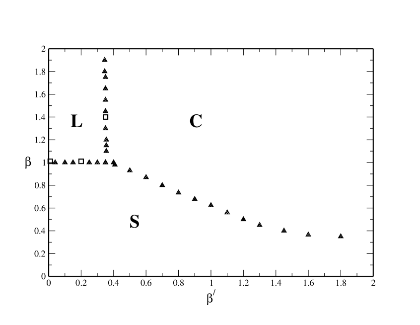
Figure 1: The phase diagram of the 5–D anisotropic U(1) gauge model.

• $W_{\mu\nu}(L_{1},L_{2})\simeq\exp(-\sigma L_{1}L_{2})$   (Confinement phase, $1\leq\mu,\nu\leq 5$))

• $W_{\mu\nu}(L_{1},L_{2})\simeq\exp(-\tau(L_{1}+L_{2}))$   (Coulomb phase, $1\leq\mu,\nu\leq 5$)

• $W_{\mu\nu}(L_{1},L_{2})\simeq\exp(-\tau^{{}^{\prime}}(L_{1}+L_{2}))$    and

• $W_{\mu T}(L_{1},L{2})\simeq exp(-\sigma^{{}^{\prime}}L_{1}L_{2})$        (Layer phase,$1\leq\mu,\nu\leq 4$.)

Moreover if we consider the helicity modulus we find that it shows the following properties:
(i) In the Strong phase (keeping $\beta^{{}^{\prime}}$ constant) the space–like helicity modulus, $h_{S}(\beta)$, takes zero value and as we approach and eventually pass the critical point it must become non-zero in the Layer phase with a value that approaches one as $\beta$ increases futher. On the other hand the transverse–like h.m., $h_{T}(\beta^{{}^{\prime}})$, must remain zero for all values of $\beta$ since both phases exhibit confinement in the fifth direction (see Section 4.1).
(ii) For the transition between the Coulomb and the Layer phase we expect for $h_{S}(\beta)$ to get a value close to one for all the values of $\beta^{{}^{\prime}}$ since the 4-dimensional layers are in a Coulomb phase, while $h_{T}(\beta^{{}^{\prime}})$ gets zero value for the Layer phase and as we pass the critical point and enter the Coulomb phase it must grow towards one as $\beta^{{}^{\prime}}$ increases (see Section 4.2).

4 Monte carlo Results

We used a 5-hit Metropolis algorithm supplemented by an overrelaxation method (see ref.[12] and references within). The lattice volumes used were: $6^{5}$, $8^{5}$, $10^{5}$, $12^{5}$ and $14^{5}$. More than $10^{5}$ sweeps were dedicated to the thermalisation process and we got samples of about $5-9\times 10^{4}$ measurements free of autocorrelation. Also two self-adjusting scales were implemented, one for the update procedure on the 4–D subspace and the other along the transverse dimension. The errors of the various measured quantities have been calculated with the jackknife method.

In the following sections we will study the Strong–Layer and the Coulomb–Layer phase transitions which are of main interest. In this work we will not study the Strong–Coulomb phase transition. However we note that strong evidence for a first order phase transition has been found due to pronounced two peak distributions (see [12]).

4.1 Strong-Layer Phase Transition

We choose a constant value for the coupling $\beta^{{}^{\prime}}=0.2$ and we let the value of $\beta$ vary for four lattice volumes $6^{5},8^{5},10^{5}~{}\mbox{and}~{}12^{5}$. For low enough values of $\beta$ the $P_{S}$ tends to values equal to $\beta/2$ according to the strong coupling expansion, then grows as it passes to the Coulomb phase tending to values equal to the weak coupling limit $1-1/(d~{}\beta)$ (see Fig.2). The transition becomes steeper as the lattice volume increases . A first evidence for a first order phase transition can be found in Fig.2 where is shown a two state signal for the space–like plaquette which persists and becomes more pronounced as we pass from lattice volume $8^{5}$ to $12^{5}$. We should note that the two–state signal is present only when we study the gauge invariant quantities measured on the four dimension layers and not on the whole volume. The reason is that as the system passes to the Layer phase with a non-continuous way the various quantities measured on the layers show a ”non-coherent” behaviour. This phenomenon, in the case of a strong first order phase transition, is responsible for producing multipeak distributions for the quantities measured on the whole five–dimensional lattice volume while for a weak first order phase transition one peak wide distributions are formed. Based on that observation and in order to obtain a more explicit signal we study the phase transition on the layer .

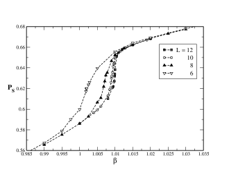
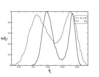
Figure 2: (a): Mean values for the space-like plaquette (the errors are included in the symbols’ size and the dashed lines guide the trend); (b): The two peak distribution $N(P_{S})$ for L=8 at $\beta^{{}^{\prime}}=0.2$ and $\beta=1.0073$ and L=12 at $\beta^{{}^{\prime}}=0.2$ and $\beta=1.0099$.

The behaviour of the space–like helicity modulus, $h_{S}$, for the same transition is depicted in Fig.3. As it was expected the $h_{S}$ takes values strictly around zero in the confinement phase and passes to non-zero values in the Coulomb phase. The transition shows a steeper passage as the lattice volume takes bigger values. In particular what is to be noticed is that for the bigger lattice volume a rather high jump arises around $\beta\sim 1.01$. In the same figure we have included the $h_{T}$ for one volume which takes zero value in both phases (shown with “uptriangles”) which is an imprint of the confinement along the fifth direction.

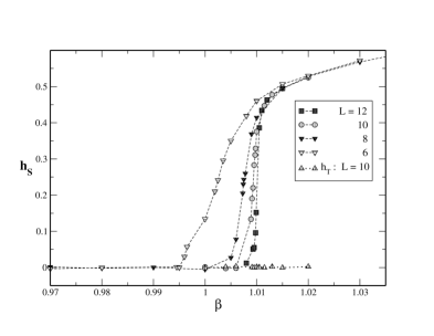
Figure 3: The volume dependence of the space–like h.m. $h_{S}$. The transverse h.m. $h_{T}$ (uptriangles) for L=10 is also shown (the errors are included in the symbols’ size and the dashed lines guide the trend).

The volume dependence of the susceptibility $S(\hat{P_{S}})$ and of the Binder cumulant, $B(\hat{P_{s}})$, are illustrated in Fig.4. The $S(\hat{P_{s}})$ (measured on the 4–D subspace according to what has been noted above) exhibits a clear increase with the volume but it is not a linear one. The minimum of the Binder cumulant also tends to increase with the volume though slowly. For the bigger lattice volume used (i.e. $12^{5}$) the minimum value, $B^{min}(\hat{P_{s}})$, seems to lie rather far from the 2/3 which should be the infinite volume limit in the case of a higher order phase transition [15].

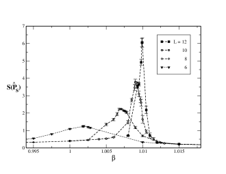
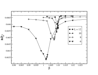
Figure 4: Volume dependence of the susceptibility (a) and of the Binder cumulant (b) for the space-like plaquette (the lines guide the trend).

We attempt to estimate the infinite volume limit for the minimum of the Binder cumulant, $B_{min}(\hat{P_{s}})$, and for that we use the ansatz:

$$B_{min}(\hat{P_{S}})=B_{min,\infty}+\sum_{k=1}^{\infty}\frac{C_{k}}{V_{4}^{k}}$$

where $V_{4}$ is for the layer volume and we limit ourselves to $k=2$. The relevant values for the fit are given in Table 1. In Fig.5 we depict the fit. The infinite volume result we obtain is: $B_{min,\infty}=0.66591(3)$ which is well far from 2/3. Note in passing that a linear fit of the three higher values gives compatible result. So we come to the conclusion that a higher order phase transition seems not to be the case.

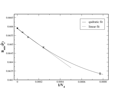
Figure 5: Fit for $B_{min}(\hat{P_{S}})$ to the infinite volume.

Now we try to apply a finite size analysis for the maxima of the susceptibility of the space–like plaquette. Following the method proposed in [16] and also applied in the 4–D U(1) gauge model in [17], we set the ansatz:

$$\beta_{c} = \beta_{\infty}+\sum_{k=1}^{\infty}\frac{A_{k}}{V_{4}^{k}}$$

$$\frac{\beta_{c}^{2}S_{max}(\hat{P}_{s})}{V_{4}} = \frac{1}{4}G_{\infty}^{2}+\sum_{k=1}^{\infty}\frac{B_{k}}{V_{4}^{k}}$$ (14)

where: $\beta_{c}$ stands for the pseudocritical value of the coupling $\beta$ at each lattice volume, $\beta_{\infty}$ is the coupling value at infinite volume and $G_{\infty}$ is the infinite volume gap in the plaquette energy. The $\beta_{c}$ values have been estimated by making a gaussian fit around the peak of the susceptibility while the use of the multihistogram method provided compatible results. The values used for the fits are given in the Table 1.

$L$	$\beta_{c}$	$B_{min}(\hat{P_{S}})$	$S_{max}(\hat{P}_{s})$	$E_{S}$	$E_{L}$
$6$	1.00180(6)	0.66335(6)	1.125( 8)	0.5925(7)	0.6484(8)
$8$	1.00710(4)	0.66483(4)	2.254(50)	0.6065(2)	0.6511(2)
$10$	1.00910(9)	0.66540(3)	3.784(40)	0.6141(2)	0.6528(1)
$12$	1.00995(3)	0.66568(2)	6.110(30)	0.6190(1)	0.6535(1)

Table 1: The pseudocritical gauge coupling values, the Binder cumulant minima, $B_{min}(\hat{P_{S}})$, the maxima of the space–like susceptibility, $S_{max}(\hat{P}_{s})$, and the energy peaks in the Strong and Layer phase for $\beta^{{}^{\prime}}=0.2$.

The results obtained from the fitting procedure with $k=2$ in Eq.(4.1) are:

$$\beta_{\infty}=1.01072(5)~{}~{}~{}\mbox{and}~{}~{}~{}G_{\infty}=0.0297(5)$$ (15)

The value for $\beta_{\infty}$ lies close to the critical value of the coupling in the 4–D U(1) gauge model found in [17]. This is rather logical since in both models there is a transition from a confinement phase to a 4-D Coulomb phase. This fact is also consistent with the assumption that the 4–D layers pass to the Coulomb phase in a more or less independent way since the transverse interaction is of a strong type.

The infinite volume gap can be measured in two additional ways. First from the double peak histograms we estimate the values of the energy peaks $E_{i=S,L}$ which correspond to the Strong and Layer phases, using independent Gaussian fits in the vicinity of each peak. Then we calculate the difference $\hat{G}=E_{L}-E_{S}$ for each lattice volume and we make use of the ansatz:

$$\hat{G}=G_{\infty}+G_{1}e^{-G_{2}L}$$ (16)

The fit is depicted in Fig.6(a). In this way we obtain the value for the infinite volume gap,

$$G_{\infty}=0.0278(13)$$ (17)

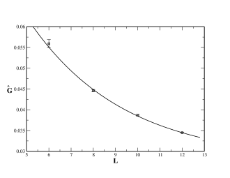
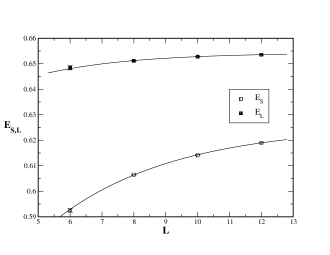
Figure 6: (a): The fit for the energy Gap, $\hat{G}$, according to the Eq.(16); (b): The fits for the energy peaks according to the Eq.(18).

Alternatively by using the energy peaks $E_{i=S,L}$ found above and given in Table 1 we perform exponential fits of the form:

$$E_{i}(L)=E_{i,\infty}+c_{1,i}e^{-c_{2,i}L}~{}~{}\mbox{where}~{}~{}i=S,~{}L$$ (18)

The results are: $E_{S\infty}=0.6257(8)$ and $E_{L\infty}=0.6543(4)$ from which we obtain the energy gap equal to:

$$G_{\infty}=0.0286(9)$$ (19)

The comparison between Eqs.(15), (17) and (19) allows the conclusion that the three different methods applied for the energy gap calculation give compatible results and safely far from zero.

It would be interesting to move to a different value of the transverse coupling in order to have a broader view of the features of the phase transition. We choose a rather small value, namely, $\beta^{{}^{\prime}}=0.01$. This choice is justified by the fact that it brings us closer to the 4–D case for which a weak first order phase transition has been found [17]. We repeat the same analysis as for the $\beta^{{}^{\prime}}=0.2$ case. The relevant values for the pseudocritical gauge couplings, the maxima of the susceptibility, the energy gap and the energy peaks $E_{S,L}$ are given in Table 2.

$L$	$\beta_{c}$	$S_{max}(P_{S})$	$E_{S}$	$E_{L}$
$6$	1.00190(8)	1.125(20)	0.5900(9)	0.6467(8)
$8$	1.00750(6)	2.210( 3)	0.6061(7)	0.6510(6)
$10$	1.00930(4)	3.710( 9)	0.6144(5)	0.6531(4)
$12$	1.01010(3)	5.980(34)	0.6189(3)	0.6336(3)

Table 2: The pseudocritical gauge coupling values, the maxima of the space–like susceptibility, $S_{max}(P_{S})$, and the values of the energy peaks in the Strong and Layer phase for $\beta^{{}^{\prime}}=0.01$.

$\beta^{{}^{\prime}}$	$\beta_{\infty}$	$G_{\infty}$
0.2	1.01072(5)	0.0297(5) / 0.0278(13) / 0.0286(9)
0.01	1.01077(5)	0.0305(20) / 0.0294(23) / 0.0303(14)

Table 3: The critical values for the space–like gauge coupling and the values for the infinite volume energy gap calculated in three ways as explained in the text, for two values of the transverse gauge coupling namely, $\beta^{{}^{\prime}}=0.2,0.01$.

Our results for both $\beta^{{}^{\prime}}=0.01$ and $\beta^{{}^{\prime}}=0.2$ can be found in Table 3 and lead to two conclusions. The first is that the phase transition occurs at almost constant value for the spatial gauge coupling $\beta$. Moreover the critical value for the transition between the 5–D confinement phase to the Layer phase lies very close to the corresponding critical value found for the 4–D U(1) gauge model. The second conclusion is that due to the non zero value for the infinite volume energy gap combined with all the rest of the analysis done, we have a clear evidence for a first order phase transition though a weak one.

4.2 Coulomb-Layer Phase Transition

We used four lattice volumes , namely: $8^{5}$,$10^{5}$,$12^{5}$ and $14^{5}$. The gauge invariant quantity used for this transition is the transverse–like plaquette whose values in the confinement phase tend to the strong coupling limit, $\beta^{{}^{\prime}}/2$, and grow as the system passes to the Coulomb phase. The space–like plaquette, as the forces on the 4–D subspace are of Coulomb type does not show any substantial change of its value (see [12]).

We choose to keep $\beta$ constant to the value 1.4 while we let $\beta^{{}^{\prime}}$ vary. In Fig.7(a) we depict the transverse–like plaquette as a function of the transverse–like coupling for four lattice volumes. One first observation is that the transition point moves to smaller values of $\beta^{{}^{\prime}}$ as the volume increases. Then there is a difference though small for the values of $P_{T}$ in the transition region between the two bigger volumes.

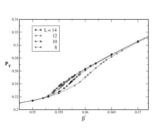
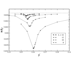
Figure 7: (a): The mean values of the transverse plaquette, $P_{T}$, with the volume; (b):The Binder cumulant, $B(\hat{P_{T}})$, as a function of the volume (the errors are included in the symbols’ size and the dashed lines guide the trend).

In Fig.7(b) we present our results for the Binder cumulant, $B(\hat{P_{T}})$, and for four lattice volumes. It can be noticed that the minimum value of the Binder cumulant for the bigger volume lies extremely close to the limit value $2/3$. Although this fact provides evidence for a continuous phase transition it can not be used as a criterion to distinguish a second order phase transition from a crossover.

The susceptibility $S(\hat{P}_{T})$ as a function of the five dimensional volume is depicted in Fig.8.

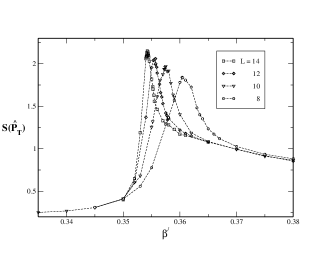
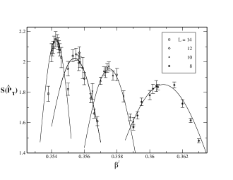
Figure 8: (a) The volume dependence of the susceptibility for the transverse-like plaquette (errorbars not shown here); (b) the same with the gaussian fits shown.

The susceptibility peaks display a small scaling with the volume. The pseudocritical $\beta^{{}^{\prime}}_{c}$ and the maxima of the susceptibility, $S_{max}(\hat{P}_{T})$, for each lattice volume have been estimated using a gaussian fit around the peak and are given in Table 4.

$L$	$\beta^{{}^{\prime}}_{c}$	$S_{max}(\hat{P}_{T})$
$8$	0.36083(8)	1.857(10)
$10$	0.35746(6)	1.940(12)
$12$	0.35541(8)	2.024(14)
$14$	0.35426(3)	2.148(15)

Table 4: The pseudocritical values $\beta^{{}^{\prime}}_{c}$ and the maxima of the transverse–like susceptibility, $S_{max}(\hat{P}_{T})$ at $\beta=1.4$.

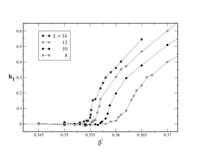
Figure 9: The volume dependence of the transverse helicity modulus (the errors are not included and the dashed lines guide the trend).

The transverse helicity modulus, $h_{T}$, offer the advantage of rendering more clear the phase transition as the lattice volume increases. In the Layer phase the force between neighbouring layers is confining, making the system insensitive to the presence of the external flux and thus giving a zero value to the ’transverse’ h.m. When the system passes to the Coulomb phase the force becomes Coulomb-like and thus $h_{T}$ obtains a non-zero value. The behaviour of the space–like h.m., $h_{S}$, is quite different: the transition from the Layer to the Coulomb phase, from the point of view of the 4–D layers, is actually a passage from a 4-D to a 5-D Coulomb law. Thus it is expected that $h_{S}$ gets a constant value . In Fig.9 the transverse helicity modulus is shown for four lattice volumes. It can be noticed that as the volume increases the transition to the Coulomb phase becomes steeper and allows, in principle, an estimation of the critical point. Indeed in comparison with the transverse–like plaquette (see Fig.7(a)) the use of the helicity modulus, $h_{T}$, helps to get a less unambigous signal of the phase transition.

Now, assuming the presence of a second order phase transition, we expect that near to the critical point the correlation length has to be given by the following expression:

$$\xi\sim|\beta^{{}^{\prime}}-\beta^{{}^{\prime}}_{c}|^{-\nu}$$ (20)

We also assume that the pseudocritical value of the transverse gauge coupling is expressed as a function of the lattice length according to the expression [18]:

$$\beta^{{}^{\prime}}(L)=\beta^{{}^{\prime}}_{\infty}(1+C_{1}L^{-\frac{1}{\nu}})$$ (21)

or equivalently by:

$$\ln|\beta(L)^{{}^{\prime}}-\beta^{{}^{\prime}}_{\infty}|=C_{2}-\frac{1}{\nu}\ln(L)$$ (22)

Using the pseudocritical values for the gauge coupling of Table 4 we obtain (see Fig.10(a)):

$$\nu=0.57(5)~{}~{}\mbox{and}~{}~{}\beta^{{}^{\prime}}_{\infty}=0.35028(53)$$ (23)

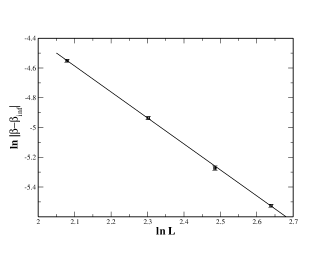
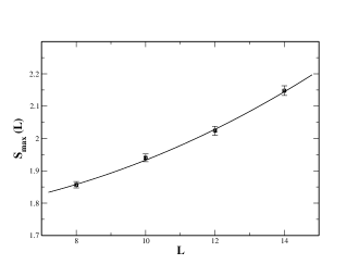
Figure 10: (a) Fit of the Eq.(22); (b) Fit of the Eq.(24).

The asymptotic scaling law for the susceptibility takes the form:

$$S_{max}(L)=C_{1}+C_{2}L^{\frac{\gamma}{\nu}}$$ (24)

Using the values of Table 4 we obtain $\frac{\gamma}{\nu}=2.19(74)$ and with the help of the Eq.(23) we get $\gamma=1.24(44)$. In the Fig.10(b) we depict the result of the fitting procedure using the Eq.(24). In other words we obtain a volume exponent equal to 0.44(15) which provides a serious evidence for a second order phase transition.

5 Conclusions

We consider a U(1) gauge model in $4+1$ dimensions with anisotropic gauge couplings. The main property of this model is the existence of a new phase which is called Layer and is characterized by Coulomb–like interaction on a 4–D subspace and confinement along the fifth direction. The other two phases of the phase diagram are a 5–D Coulomb phase and a confinement phase. The study of the phase transitions reveals that the Layer and the Confinement phases are separated by a weak first order phase transition whose critical gauge coupling is found very close to the Coulomb–confinement critical coupling of the 4–D model. Furthermore for the Layer–Coulomb phase transition we provide serious evidence of a second order phase transition. If this conclusion persists after the use of bigger lattice volumes it would provide a promising scenario for a gauge field localization based on a model that features a continuum limit.

A final remark should be added which has to do with a possible connection of our 5–D gauge model with the percolation model. In [19],[20], it is argued that percolation in three dimensions can be viewed as a gauge theory and it can capsulate most of the features of confinement and the glueball spectrum. The values of the exponents $\gamma$ and $\nu$ given at the end of the Section 4.2 are in a good agreement with the values of the corresponding exponenents of the 5–D percolation model which are: $\gamma_{5Dperc}=1.18$ and $\nu_{5Dperc}=0.57$ (see [21]). Although this fact alone can not justify any further argumentation on a possible universality class issues, however it might be useful in providing a new point of view for the confinement mechanism along the extra dimension.

6 Acknowledgements

We acknowledge support from the EPEAEK programme “Pythagoras II” co-funded by the European Union (75%) and the Hellenic State (25%). We are grateful to K. Anagnostopoulos and G. Koutsoumbas for reading and discussing the manuscript and making useful comments.

References

- [1] I. Antoniadis, Phys. Lett. B246 (1990)377; N. Arkani-Hamed, S. Dimopoulos and G. Dvali, Phys. Lett. B429 (1998)263, [hep-th/9803315]; I. Antoniadis, N. Arkani-Hamed, S. Dimopoulos and G. Dvali, Phys. Lett. B436 (1998)257, [hep-th/9804398].
- [2] L.Randall and R.Sundrum, Phys. Rev. Lett. 83 (1999) 4690, [hep-th/9906064]; Phys. Rev. Lett.83(1999)3370, [hep-ph/9905221].
- [3] V.A. Rubakov, Usp.Fiz.Nauk 171 913-938 (2001), [hep-ph/0104152].
- [4] C. Csàki, TASI Lectures on Extra Dimensions and Branes, [hep-ph/0404096].
- [5] R. Sundrum, TASI 2004 Lectures: To the Fifth Dimension and Back, [hep-th/0508134].
- [6] V.A. Rubakov and M. Shaposhnikov, Phys. Lett. B125, 136 (1983); R.Jackiw and C.Rebbi, Phys. Rev. D13, 3398 (1976); R.Jackiw and P. Rossi, Nucl. Phys. B190, 681 (1981); D. B. Kaplan,Phys. Lett. B288, 342 (1992) [hep-lat/9206013]; T. Gherghetta and A. Pomarol, Nucl. Phys. B586, 141 (2000) [hep-th/0003129]; A. Kehagias and K. Tamvakis, Phys. Lett. B504, 38 (2001) [hep-th/0010112].
- [7] G.R. Dvali and M.A. Shifman, Phys. Lett. B396, 64 (1997) [hep-th/9612128].
- [8] P. Dimopoulos, K. Farakos and G. Koutsoumbas, Phys. Rev. D65:074505 (2002) [hep-lat/0111047].
- [9] K. Farakos and P. Pasipoularides, Phys. Lett. B621, 224 (2005) [hep-th/0504014]; Phys. Rev. D73:084012 (2006) [hep-th/0602200].
- [10] Y.K. Fu and H.B. Nielsen, Nucl. Phys. B 236, 167 (1984); Nucl. Phys. B254, 127 (1985).
- [11] C.P. Korthals-Altes, S. Nicolis and J. Prades, Phys. Lett. B316 339 (1993) [hep-lat/9306017]; A. Hulsebos, C.P. Korthals-Altes and S. Nicolis, Nucl. Phys. B450 437 (1995) [hep-th/9406003].
- [12] P. Dimopoulos, K. Farakos, A. Kehagias and G. Koutsoumbas, Nucl.Phys.B617:237-252,2001 [hep-th/0007079] .
- [13] M. Vettorazzo and P. Forcrand Nucl.Phys.Proc.Suppl.129:739-741,2004 [hep-lat/0311007]; Nucl.Phys. B686: 85-118,2004 [hep-lat/0311006]; Phys.Lett. B604: 82-90,2004 [hep-lat/0409135].
- [14] P. Dimopoulos and K. Farakos, Phys. Rev. D70, 045005 (2004) [hep-ph/0404288]; P.Dimopoulos, K.Farakos and S. Nicolis, Eur. Phys. J. C24, 87, (2002) [hep-lat/0105014].
- [15] K. Binder and D.H Heermann, Monte Carlo Simulation in Statistical Physics, Springer–Verlag, 1992.
- [16] C.Borgs, R.Kotecky Phys.Rev.Lett.68:1734-1737,1992 ; C.Borgs, R.Kotecky and Miracle-Sole J.Stat.Phys. 62 529,1991.
- [17] G. Arnold, B.Bunk, T. Lippert and K. Schilling Nucl.Phys.Proc.Suppl.119:864-866,2003 [hep-lat/0210010]; G. Arnold, T. Lippert, K. Schilling and T. Neuhaus Nucl.Phys.Proc.Suppl.94:651-656,2001. [hep-lat/0011058].
- [18] M.E.J. Newman and G.T. Barkema, Monte Carlo Methods in Statistical Physics, Chapter 8, Oxford University Press, 1999.
- [19] F. Gliozzi, S. Lottini, M. Panero and A. Rago, Nucl. Phys. B719:255, 2005 [cond-mat/0502339]; S. Lottini and F. Gliozzi PoSLAT2005:292, 2006 [hep-lat/0601011]; F.Gliozzi, Where is the confining string in random percolation [hep-lat/0510034].
- [20] R. Ziff, A Simple Algorithm to test for linking to Wilson Loops in percolation [cond-mat/0504260].
- [21] J. Adler, Y. Meir, A. Aharony, A.B. Harris, Phys. Rev. B41: 9183, 1990.