ROM2F/2006-17, CERN-PH-TH/2006-131, FTUV-06-2007

IFIC/06-29, MKPH-T-06-14, DESY 06-112

July 2006

Non-perturbative renormalisation of left-left

four-fermion operators with Neuberger fermions

P. Dimopoulos^a, L. Giusti^b, P. Hernández^c, F. Palombi^d†,

C. Pena^b†, A. Vladikas^a†, J. Wennekers^e and H. Wittig^d†

^a INFN, Sezione di Roma “Tor Vergata”

c/o Dipartimento di Fisica, Università di Roma “Tor Vergata”

Via della Ricerca Scientifica 1, I-00133 Rome, Italy

^b CERN, Physics Department, TH Division

CH-1211 Geneva 23, Switzerland

^c Dpto. de Física Teórica and IFIC, Universitat de València

E-46100 Burjassot, Spain

^d Institut für Kernphysik, University of Mainz

D-55099 Mainz, Germany

^e DESY, Theory Group

Notkestraße 85, D-22603 Hamburg, Germany

 Abstract We outline a general strategy for the non-perturbative renormalisation of composite operators in discretisations based on Neuberger fermions, via a matching to results obtained with Wilson-type fermions. As an application, we consider the renormalisation of the four-quark operators entering the $\Delta S=1$ and $\Delta S=2$ effective Hamiltonians. Our results are an essential ingredient for the determination of the low-energy constants governing non-leptonic kaon decays.  

1 Introduction

The renormalisation of four-fermion operators is an essential ingredient in lattice QCD computations of weak matrix elements. In this letter we will address the logarithmically divergent renormalisation of left-left four-quark operators, with an emphasis on the $\Delta S=1$ effective Hamiltonian governing non-leptonic kaon decays.

The treatment of $\Delta S=1$ weak decays via an effective weak Hamiltonian with an active charm quark has been recently reviewed in [1]. After performing the operator product expansion and neglecting top quark effects, which are suppressed by three orders of magnitude relative to the contributions of up and charm quarks, the expression found for the $\Delta S=1$ effective weak Hamiltonian in the formal continuum theory is

$${\cal H}_{\rm w}=\frac{g_{\rm w}^{2}}{4M_{W}^{2}}(V_{us})^{*}V_{ud}\sum_{\sigma=\pm}\{k_{1}^{\sigma}{\cal Q}_{1}^{\sigma}+k_{2}^{\sigma}{\cal Q}_{2}^{\sigma}\}\,.$$ (1.1)

In the above expression $g_{\rm w}=4\sqrt{2}G_{\rm F}M_{W}^{2}$, $k_{1,2}^{\sigma}$ are Wilson coefficients, and the dimension-six operators ${\cal Q}_{1,2}^{\sigma}$ have the form

$${\cal Q}_{1}^{\pm} =[(\bar{s}\gamma_{\mu}P_{-}u)(\bar{u}\gamma_{\mu}P_{-}d)\pm(\bar{s}\gamma_{\mu}P_{-}d)(\bar{u}\gamma_{\mu}P_{-}u)]-[u~{}\rightarrow~{}c]\,,$$ (1.2)

$${\cal Q}_{2}^{\pm} =(m_{u}^{2}-m_{c}^{2})\{m_{d}(\bar{s}P_{+}d)+m_{s}(\bar{s}P_{-}d)\}\,,$$ (1.3)

where parentheses around quark bilinears indicate colour and spin traces and $P_{\pm}={\scriptstyle{{1\over 2}}}(\mathbf{1}\pm\gamma_{5})$. Although our procedure is completely general, we will from now on concentrate in the ${\rm SU}(4)_{\rm L}\times{\rm SU}(4)_{\rm R}$ symmetric limit, where all quark masses are degenerate [1]. In this limit the only contribution to decay amplitudes comes from matrix elements of the operators ${\cal Q}_{1}^{\pm}$. Moreover, the operator renormalisation pattern is greatly simplified, as mixing with lower dimension operators is absent. We stress, however, that our results, being obtained in a mass-independent renormalisation scheme, will renormalise properly subtracted operators also beyond the ${\rm SU}(4)_{\rm L}\times{\rm SU}(4)_{\rm R}$ symmetric limit.

Our strategy to renormalise ${\cal Q}^{\pm}_{1}$ is similar to the technique proposed in [2] for the computation of the renormalised chiral condensate. It involves matching bare correlation functions (or matrix elements) computed with Neuberger fermions to their renormalisation group invariant (RGI) counterparts. The latter are computed in the continuum limit with some variant of Wilson fermions, for which mature techniques for fully non-perturbative renormalisation exist. Our choice will be twisted mass QCD (tmQCD) with an $\mbox{O}(a)$ improved fermion action.

Although we will concentrate specifically on the operators of the $\Delta S=1$ Hamiltonian, both the proposed methodology and our results have a wider range of application. In particular, the renormalisation factors that we will obtain for ${\cal Q}^{+}_{1}$ renormalise also the four-fermion operator entering the $\Delta S=2$ effective Hamiltonian. In the present work, all computations are performed in the quenched approximation.

In the next section we will describe the strategy of the computation. In section 3 we discuss the computation of RGI operators in the continuum limit, based on a twisted mass QCD (tmQCD) Wilson fermion regularisation. In section 4 we discuss our results with Neuberger fermions, and compute non-perturbative renormalisation factors. Section 5 deals with perturbative estimates of the same renormalisation factors. We present our conclusions in section 6.

2 Strategy

Let us consider a generic multiplicatively renormalisable operator. The notation will follow closely that of [1]. We will be dealing only with mass-independent renormalisation schemes.

We start by recalling the definition of renormalisation group invariant (RGI) composite operators. The RGI insertion of a local operator ${\cal Q}$ into a continuum on-shell correlation function is given by

$$\begin{split}\hat{{\cal Q}}(g_{\rm R},m_{{\rm R}},L)&=c_{\rm s}(\mu/\Lambda)\,\lim_{a\rightarrow 0}Z_{\rm s}(g_{0},a\mu)\,{\cal Q}(g_{0},m_{0},L)\\ &\equiv\lim_{a\rightarrow 0}\hat{Z}(g_{0})\,{\cal Q}(g_{0},m_{0},L)\,,\end{split}$$ (2.4)

where $Z_{\rm s}$ is a renormalisation constant that renders the operator finite, $\Lambda$ is the QCD scale, and $g_{0},m_{0}$ ($g_{\rm R},m_{{\rm R}}$) denote the bare (renormalised) gauge coupling and quark mass(es). The subscript “${\rm s}$” labels the renormalisation scheme. We have also indicated explicitly that correlation functions will be computed in a finite volume of spatial size $L$ (eventually taking $L\to\infty$). The RG-evolution function is given by

$$c_{\rm s}(\mu/\Lambda)=\left[2b_{0}\kern 1.0pt\overline{\kern-1.0ptg\kern 0.0pt}\kern 1.0pt^{2}(\mu)\right]^{\gamma_{0}/(2b_{0})}\exp\left\{-\int_{0}^{\kern 1.0pt\overline{\kern-1.0ptg\kern 0.0pt}\kern 1.0pt(\mu)}{\rm d}g\left[\frac{\gamma(g)}{\beta(g)}+\frac{\gamma_{0}}{b_{0}g}\right]\right\}\,,$$ (2.5)

where we have used the perturbative expansions of the anomalous dimension of the operator $\gamma$ and the $\beta$-function, viz.

$$\beta(g)\stackrel{{\scriptstyle g\to 0}}{{\approx}}-g^{3}(b_{0}+b_{1}g^{2}+\ldots)\,,~{}~{}~{}~{}~{}~{}~{}\gamma(g)\stackrel{{\scriptstyle g\to 0}}{{\approx}}g^{2}(\gamma_{0}+\gamma_{1}g^{2}+\ldots)\,.$$ (2.6)

It has to be stressed that the (scale-independent) RGI renormalisation factor $\hat{Z}(g_{0})\equiv c_{\rm s}(\mu/\Lambda)Z_{\rm s}(g_{0},a\mu)$ depends on the renormalisation scheme only via cutoff effects, since the RGI operator insertion $\hat{{\cal Q}}$ is scheme-independent. On the other hand, $\hat{Z}$ is regularisation-dependent. We also stress that the running factor $c_{\rm s}$ is a continuum quantity, and hence regularisation-independent.

We now consider two different lattice regularisations, namely Wilson (denoted by “w”) and Neuberger (or overlap) fermions (denoted by “ov”). Our aim is to construct RGI renormalisation factors for Neuberger fermions operators by matching renormalised quantities in both regularisations. The first step consists of using the first regularisation in order to compute the RGI operator $\hat{{\cal Q}}$ at a reference physical point, parametrised here by $({g_{\rm R}}_{,\rm ref},m_{{\rm R},\rm ref},L_{\rm ref})$, viz.

$$\hat{{\cal Q}}({g_{\rm R}}_{,\rm ref},m_{{\rm R},\rm ref},L_{\rm ref})=\lim_{a\to 0}\hat{Z}^{\rm w}(g_{0})\,{\cal Q}^{\rm w}(g_{0},m_{0},L_{\rm ref})\,.$$ (2.7)

It is essential to note that any reference to the regularisation employed in the r.h.s. of eq. (2.7) has disappeared after the continuum limit has been taken. The second step consists of tuning a point $(g^{\prime}_{0},m^{\prime}_{0})$ in the bare parameter space of the second regularisation, which corresponds to the same values of the renormalised parameters $({g_{\rm R}}_{,\rm ref},m_{{\rm R},\rm ref})$. Assuming universality of the continuum limit, one then has

$$\begin{split}\hat{{\cal Q}}({g_{\rm R}}_{,\rm ref},m_{{\rm R},\rm ref},L_{\rm ref})&=\hat{Z}^{\rm ov}(g_{0}^{\prime})\,{\cal Q}^{\rm ov}(g^{\prime}_{0},m^{\prime}_{0},L_{\rm ref})\,+\mbox{O}(a^{2})\,,\end{split}$$ (2.8)

where we have explicitly used the fact that correlation functions computed with Neuberger fermions exhibit scaling violations of at most $\mbox{O}(a^{2})$. Once the bare quantity ${\cal Q}^{\rm ov}(g^{\prime}_{0},m^{\prime}_{0},L_{\rm ref})$ has been computed, eq. (2.8) yields $\hat{Z}^{\rm ov}(g_{0}^{\prime})$, provided that $\hat{{\cal Q}}({g_{\rm R}}_{,\rm ref},m_{{\rm R},\rm ref},L_{\rm ref})$ has been determined through eq. (2.7). This procedure can be repeated at several bare couplings and masses $(g^{\prime}_{0},m^{\prime}_{0})$, always corresponding to $({g_{\rm R}}_{,\rm ref},m_{{\rm R},\rm ref})$; in this way the lattice spacing may be varied, while the physics (i.e. physical volume and renormalised coupling and masses) is kept fixed. Note that Eq. (2.8) is to be interpreted as a renormalisation condition that implicitly defines a mass-independent renormalisation scheme. Thus it ensures that the RGI renormalisation factors computed in this way will correctly renormalise the operators at any value of the quark masses $m_{{\rm R}}$. In particular, $\hat{Z}^{\rm ov}$ depends on quark masses only via cutoff effects (though it is not guaranteed a priori that such dependence is small). On the other hand, the renormalisation prescription (2.8) reproduces by construction the RGI result at the reference point for any chosen set of bare parameters. Thus the procedure is only useful if the targeted physical regime, characterised by $(g_{\rm R},m_{{\rm R}},L)$, is well away from $({g_{\rm R}}_{,\rm ref},m_{{\rm R},\rm ref},L_{\rm ref})$.

The present work provides an application of this strategy. The ultimate aim, which is achieved in ref. [3], is the computation of the effective low-energy couplings governing non-leptonic kaon decays, following the strategy described in [1]. This involves the computation, carried out using Neuberger fermions, of the chiral limit values of the ratios of correlation functions

$$R^{\pm}_{1}(x_{0},y_{0})=\frac{\langle[J_{0}(x)]_{du}{\cal Q}_{1}^{\pm}(0)[J_{0}(y)]_{us}\rangle}{\langle[J_{0}(x)]_{du}[J_{0}(0)]_{ud}\rangle\langle[J_{0}(0)]_{su}[J_{0}(y)]_{us}\rangle}\,,$$ (2.9)

where $J_{\mu}$ is the left-handed current

$$[J_{\mu}(x)]_{\alpha\beta}=\bar{\psi}_{\alpha}\gamma_{\mu}P_{-}\psi_{\beta}\,,$$ (2.10)

and $\alpha,\beta$ are flavour indices. An essential ingredient of the procedure are the renormalisation factors $[\hat{Z}_{1}^{\pm}/Z_{\rm\scriptscriptstyle A}^{2}]$, the computation of which is the goal of the present work.

In order to compute non-perturbatively the renormalisation factors $[\hat{Z}_{1}^{\pm}/Z_{\rm\scriptscriptstyle A}^{2}]$ for Neuberger fermions, we will employ the ratios of QCD matrix elements

$${\cal R}_{\pm}\equiv\frac{\langle\pi^{+}|{\cal Q}_{1}^{\pm}|K^{+}\rangle}{\langle\pi^{+}|J_{0}|0\rangle\langle 0|J_{0}|K^{+}\rangle}\,$$ (2.11)

computed in large volumes and at a value of the reference quark mass $m_{{\rm R},{\rm ref}}$ corresponding to $m_{\rm PS}=m_{\pi}=m_{K}=m_{K}^{\rm phys}=495~{}{\rm MeV}$. Note that, in the ${\rm SU}(4)_{\rm L}\times{\rm SU}(4)_{\rm R}$ symmetric limit, the ratio ${\cal R}_{+}$ will be equal, up to a trivial factor, to the Kaon bag parameter $B_{K}$. The RGI ratios $\hat{{\cal R}}_{\pm}$ will be computed, as in Eq. (2.7), using a Wilson fermion regularisation. To this purpose, we will compute the bare quantities ${\cal R}_{\pm}$ at several values of the bare coupling $g_{0}$, and use the RGI renormalisation factors computed in the same $g_{0}$ range in [4], using a Schrödinger Functional (SF) framework. We will then apply Eq. (2.8) to match the RGI ratios $\hat{{\cal R}}_{1}^{\pm}$ to the ratios of bare matrix elements computed with Neuberger fermions. Since the matching reference regime of large volumes and meson masses of the order of $m_{K}^{\rm phys}$ is well away from the target one in which $[\hat{Z}^{\pm}/Z_{\rm\scriptscriptstyle A}^{2}]$ are to be used, the construction is indeed non-trivial. In this way we have exploited the fact that Wilson fermions are well suited for simulations in the strange-quark regime, while they become problematic close to the chiral limit, where Neuberger fermions are clearly advantageous.

For the sake of consistency, we will also perform a direct determination of the ratio $\hat{Z}_{1}^{+;\rm ov}/\hat{Z}_{1}^{-;\rm ov}$, computed from a matching involving the ratio of matrix elements

$$\frac{{\cal R}_{+}}{{\cal R}_{-}}=\frac{\langle\pi^{+}|{\cal Q}_{1}^{+}|K^{+}\rangle}{\langle\pi^{+}|{\cal Q}_{1}^{-}|K^{+}\rangle}\,.$$ (2.12)

This specific ratio is of particular interest, as it enters directly the study of the $\Delta I=1/2$ enhancement rule.

Some comments are in order. The renormalisation factors obtained via the procedure just described do not lead, obviously, to independent renormalised values for the ratios of matrix elements in Eq. (2.11) computed at the reference point $m_{K}^{\rm phys}$, as a tautology would result. As explained above, the renormalisation factors $[\hat{Z}_{1}^{\pm}/Z_{\rm\scriptscriptstyle A}^{2}]$ will rather be used to renormalise quantities effectively computed in the chiral limit. They can also be used e.g. to renormalise ratios of correlation functions computed in the $\epsilon$-regime. The fact that the matching involves correlation functions computed with both periodic and SF boundary conditions does not, on the other hand, give rise to any subtlety, as only hadronic matrix elements computed in a large volume are involved.

Unlike the above strategy, adopted in this work, the ideal matching procedure should not involve the tradeoff of a long-distance matrix element of physical relevance. It is e.g. possible to match a different matrix element of the same operator, or to take a reference point for the matching which is well away from all the target physical regimes of interest. On the other hand, the particular strategy adopted here has the advantage that it allows to use the numerical results obtained in the context of [5].

3 Wilson-tmQCD computation of RGI operators

We will now discuss the computation of the RGI operators $\hat{{\cal Q}}_{1}^{\pm}$ (i.e. the l.h.s. of Eq. (2.8)), using the tmQCD formalism with Wilson quarks [6].

We start by recalling that, with Wilson fermions, the renormalisation of ${\cal Q}_{1}^{\pm}$ is more subtle than in chirally symmetric regularisations (see [7] for a detailed discussion). Customarily, both operators are split into parity-even and parity-odd parts as

$${\cal Q}_{1}^{\pm}={\cal Q}^{\pm}_{\rm VV+AA}-{\cal Q}^{\pm}_{\rm VA+AV}\,,$$ (3.13)

in standard notation. In the three-point correlation functions considered below, parity conservation in QCD ensures that the only contribution comes from the parity-even part ${\cal Q}^{\pm}_{\rm VV+AA}$. With ordinary Wilson fermions, as a consequence of the breaking of chiral symmetry, the renormalisation of ${\cal Q}^{\pm}_{\rm VV+AA}$ requires the subtraction of four finite counterterms involving all the remaining Lorentz-invariant, parity-even four-quark operators with the same flavour structure. On the other hand, it is possible to construct twisted mass QCD (tmQCD) Wilson regularisations in which the counterterms are absent, and the operator renormalises multiplicatively. The basic property that has to be satisfied is that the chiral rotation of the quark fields that generates the twisted mass term maps ${\cal Q}^{\pm}_{\rm VV+AA}$ onto ${\cal Q}^{\pm}_{\rm VA+AV}$. In mass-independent renormalisation schemes, the latter is protected from mixing with other four-fermion operators by CPS symmetry. Examples of such regularisations have been discussed in [8].

Here we will adopt, however, a different approach, which will allow us to use the numerical results obtained in [5]. To that purpose we restrict ourselves to the quenched approximation, and use the formalism for valence quark flavours advocated in [9]. We consider a theory with six valence flavours, that we will label $\psi=(u,d,s,c,u^{\prime},c^{\prime})^{T}$. We will employ two tmQCD regularisations, characterised by the choice of twist angle $\alpha$ in the definition of the fermion action:

$$S^{(\alpha)}_{\rm tmQCD}=a^{4}\sum_{x,y}\bar{\psi}(x)\left\{D_{\rm w,sw}+\mathbf{m}^{(\alpha)}+i\gamma_{5}\boldsymbol{\mu}^{(\alpha)}\right\}(x,y)\,\psi(y)\,,$$ (3.14)

where $D_{\rm w,sw}$ is the Wilson operator with a Sheikholeslami-Wohlert term, $\mathbf{m}^{(\alpha)}$ and $\boldsymbol{\mu}^{(\alpha)}$ are diagonal mass matrices, and the label $\alpha$ refers to the twist angle entering chiral rotations. The bare mass parameters are tuned so that, up to $\mbox{O}(a^{2})$ corrections, the renormalised mass matrices have the form

$$\mathbf{m}^{(\pi/2)}_{\rm R} =M_{\rm R}\,{\rm diag}(0,0,1,0,1,1)\,,~{}~{}~{}~{} \boldsymbol{\mu}^{(\pi/2)}_{\rm R} =M_{\rm R}\,{\rm diag}(1,1,0,1,0,0)\,,$$ (3.15)

$$\mathbf{m}^{(\pi/4)}_{\rm R} =\frac{M_{\rm R}}{\sqrt{2}}\,{\rm diag}(1,1,1,1,1,1)\,,~{}~{}~{}~{} \boldsymbol{\mu}^{(\pi/4)}_{\rm R} =\frac{M_{\rm R}}{\sqrt{2}}\,{\rm diag}(1,1,-1,1,-1,-1)\,,$$ (3.16)

where $M_{\rm R}$ is the physical renormalised quark mass. The mass tuning procedure is identical to the one described in [5]. We then introduce the operators

$$\begin{split}\widetilde{\cal Q}_{1}^{\pm}=&[(\bar{s}\gamma_{\mu}P_{-}u)(\bar{u}^{\prime}\gamma_{\mu}P_{-}d)\pm(\bar{s}\gamma_{\mu}P_{-}d)(\bar{u}^{\prime}\gamma_{\mu}P_{-}u)]-[u\rightarrow c\,,\,u^{\prime}\rightarrow c^{\prime}]\,.\end{split}$$ (3.17)

Using the standard relation between QCD and tmQCD in the continuum limit, one finds, for the two regularisations specified above, that the following equalities hold between operator insertions in RGI correlation functions

$$[\hat{\widetilde{\cal Q}}_{\rm VV+AA}^{\pm}]_{\rm QCD}=i\,[\hat{\widetilde{\cal Q}}_{\rm VA+AV}^{\pm}]_{\rm tmQCD}\,,$$ (3.18)

$$Z_{\rm\scriptscriptstyle A}[A_{\mu}]_{su,{\rm QCD}}=\frac{1}{\sqrt{2}}\left\{Z_{\rm\scriptscriptstyle A}[A_{\mu}]_{su,{\rm tmQCD}}-iZ_{\rm\scriptscriptstyle V}[V_{\mu}]_{su,{\rm tmQCD}}\right\}\,,$$ (3.19)

$$Z_{\rm\scriptscriptstyle A}[A_{\mu}]_{du^{\prime},{\rm QCD}}=\frac{1}{\sqrt{2}}\left\{Z_{\rm\scriptscriptstyle A}[A_{\mu}]_{du^{\prime},{\rm tmQCD}}-iZ_{\rm\scriptscriptstyle V}[V_{\mu}]_{du^{\prime},{\rm tmQCD}}\right\}\,,$$ (3.20)

where $[A_{\mu}]_{\alpha\beta}=\bar{\psi}_{\alpha}\gamma_{\mu}\gamma_{5}\psi_{\beta}$ and $[V_{\mu}]_{\alpha\beta}=\bar{\psi}_{\alpha}\gamma_{\mu}\psi_{\beta}$. The current normalisations $Z_{\rm\scriptscriptstyle A},Z_{\rm\scriptscriptstyle V}$, as well as the $\mbox{O}(a)$ improvement coefficient $c_{\rm\scriptscriptstyle A}$ needed to construct an $\mbox{O}(a)$ improved axial current, are set to the values computed by the Alpha Collaboration [10, 11].

Correlation functions are computed within a Schrödinger functional (SF) framework, with quark and gluon fields obeying periodic boundary conditions in space (with period $L$) and (homogeneous) Dirichlet boundary conditions in time at the hypersurfaces $x_{0}=0$ and $x_{0}=T$. Ratios of correlation functions, from which the ratios of matrix elements ${\cal R}_{\pm}$ and ${\cal R}_{+}/{\cal R}_{-}$ can be extracted, are defined in complete analogy to the ones specified for the extraction of $B_{K}$ in [5]. Our run parameters, too, are the same as in [5], and are listed in Tables 1 and 5 of that work, save for one important exception, concerning the dataset at $\beta=6.1$. After completion of ref. [5], its authors carried out a proper determination of $\kappa_{\rm cr}(\beta=6.1)$, based on the method of [10]. They found that this estimate of $\kappa_{\rm cr}$ disagrees by several standard deviations from the value cited in the literature [12], which had been used in [5] for the tuning of the bare mass parameters. This discrepancy hence necessitated a new determination of the bare mass parameters in order to satisfy the constraints imposed by the prescribed values of the twist angles. Consequently, the runs at $\beta=6.1$ had to be repeated after completion of [5]. Full details will be provided separately [14]. In the present work we merely quote the corrected value of ${\cal R}_{+}$ in the continuum limit.

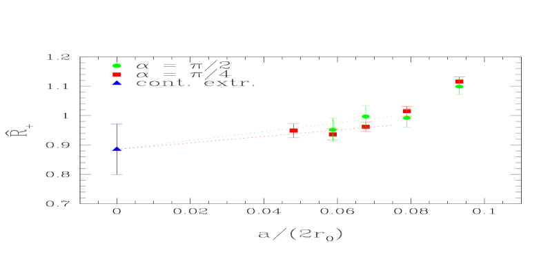
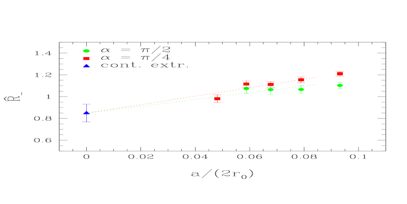
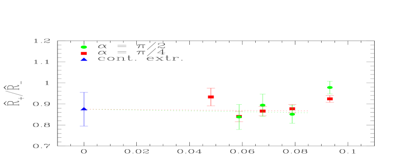
Figure 1: Continuum limit extrapolations of $\hat{{\cal R}}^{\pm}$ and $\frac{\hat{{\cal R}}^{+}}{\hat{{\cal R}}^{-}}$.

The RGI ratios are obtained upon multiplication by the RGI renormalisation factors $\hat{Z}_{\rm VA+AV}^{\pm}$. The latter have been computed non-perturbatively in [4], using the standard SF finite-size scaling analysis, for a range of inverse couplings $6.0\lesssim\beta\lesssim 6.5$. Out of the various SF renormalisation schemes considered in [4] we have chosen to employ scheme 1 for the renormalisation of $\widetilde{\cal Q}_{\rm VA+AV}^{+}$ and scheme 8 for $\widetilde{\cal Q}_{\rm VA+AV}^{-}$; the reasons are explained in [4] and [13]. The appropriate error analysis has been extensively discussed (for $\hat{{\cal R}}_{+}$) in [5]. The continuum limit is then obtained by performing a combined extrapolation of the results coming from both tmQCD regularisations. The extrapolation is linear in the lattice spacing $a$, since the four-fermion operator is not $\mbox{O}(a)$ improved, and hence the leading lattice artifacts in ${\cal R}_{\pm}$ are expected to be $\mbox{O}(a)$. Furthermore, as discussed in [5], at the lowest values of $\beta$ the $\mbox{O}(a)$ ambiguity in the determination of the improvement coefficient $c_{\rm\scriptscriptstyle A}$ has a significant impact on cutoff effects. Under these premises, our most stable continuum limit extrapolation for $\hat{{\cal R}}_{+}$ is obtained by discarding the $\beta=6.0,6.1$ data points, while for $\hat{{\cal R}}_{-}$ and $\hat{{\cal R}}_{+}/\hat{{\cal R}}_{-}$ only $\beta=6.0$ is discarded. The final results, illustrated in Fig. 1, are

$$\hat{{\cal R}}_{+}=0.885(86)\,,~{}~{}~{}~{}~{}~{}~{}~{}~{}~{}~{}\hat{{\cal R}}_{-}=0.849(82)\,,$$ (3.21)

$$\frac{\hat{{\cal R}}_{+}}{\hat{{\cal R}}_{-}}=0.875(80)\,.$$ (3.22)

We stress that the volume dependence of these results is well within the quoted uncertainties (see [5] for details).

Eqs. (3.21-3.22) are the main result of the present work. In the next section we will use them to determine the renormalisation factors needed with Neuberger fermions. It must be stressed at this point that the continuum limit extrapolation is rather long and, in the case of $\hat{{\cal R}}_{-}$, strongly driven by the $\beta=6.45$ datum. A better control of the continuum limit extrapolations could be achieved e.g. by removing $\mbox{O}(a)$ effects as suggested in ref [9]. This is beyond the scope of the present letter.

4 Renormalisation constants for Neuberger fermions

Having constructed the RGI ratios of matrix elements in eq. (2.11), we now insert them in Eq. (2.8) and solve for the Neuberger fermions renormalisation constants $\hat{Z}_{1}^{\pm,\rm ov}(g_{0})$.

In order to regularise the theory using Neuberger fermions, we start by introducing the Neuberger-Dirac operator [15]

$$D=\frac{1}{\bar{a}}\left\{\mathbf{1}-A(A^{\dagger}A)^{-1/2}\right\}\,,~{}~{}~{}~{}~{}~{}~{}A=1+s-aD_{\rm w}\,,$$ (4.23)

where $D_{\rm w}$ is the massless Wilson-Dirac operator, $a$ denotes the lattice spacing, and $s$ is a free parameter in the range $|s|<1$. By setting $\bar{a}=a/(1+s)$ it is straightforward to check that $D$ satisfies the Ginsparg-Wilson relation

$$\gamma_{5}D+D\gamma_{5}=\bar{a}D\gamma_{5}D\,.$$ (4.24)

Composite operators which have proper chiral transformation properties in the regularised theory are obtained by performing the substitution

$$\begin{aligned} \psi&\to\left(\mathbf{1}-{\scriptstyle{{1\over 2}}}\bar{a}D\right)\psi\,,\\ \bar{\psi}&\to\bar{\psi}\,.\end{aligned}$$

The operators ${\cal Q}_{1}^{\pm}$ in the discretised theory share the same transformation properties under chiral symmetry as their counterparts in the continuum (see [1] and references therein).

$\beta$	$am$	$r_{0}m_{\rm PS}$	${\cal R}^{\rm ov}_{+}$	${\cal R}^{\rm ov}_{-}$	${\cal R}^{\rm ov}_{+}/{\cal R}^{\rm ov}_{-}$
$5.8485$	$0.060$	$1.259(10)$	$0.772(30)$	$1.514(73)$	0.511(28)

Table 1: Results with Neuberger fermions, obtained on a $16^{3}\times 32$ lattice from 197 configurations and using low-mode averaging with 20 low modes of the Neuberger-Dirac operator. The physical spatial extent of the lattice is $L/(2r_{0})=1.98$.

Bare values for the ratios of matrix elements ${\cal R}_{\pm}$, are extracted from the ratios of correlation functions of eq. (2.9). The details of the computation, performed at a fixed value of $\beta$ with periodic boundary conditions in all Euclidean spacetime directions, are reported in [1, 16, 3]. The simulation parameters and our results for ${\cal R}_{\pm}$ are provided in Table 1. Since our pseudoscalar mass is compatible within errors with the kaon mass $r_{0}m_{K}^{\rm phys}=1.2544$, there is no need to consider other values of the quark mass to inter/extrapolate the kaon point. Again, finite volume effects are expected to lie within the quoted uncertainties.

Finally, by combining the continuum limit results of Eqs. (3.21-3.22) with the bare Neuberger fermions results of Table 1 we derive non-perturbative estimates of the RGI renormalisation factors

$$\left.\frac{\hat{Z}_{1}^{\pm}}{Z_{\rm\scriptscriptstyle A}^{2}}\right|_{\beta=5.8485}=\frac{\hat{{\cal R}}_{\pm}}{{\cal R}_{\pm}^{\rm ov}}\,,~{}~{}~{}~{}~{}~{}~{}~{}~{}\left.\frac{\hat{Z}_{1}^{-}}{\hat{Z}_{1}^{+}}\right|_{\beta=5.8485}=\frac{{\cal R}_{+}^{\rm ov}/{\cal R}_{-}^{\rm ov}}{\hat{{\cal R}}_{+}/\hat{{\cal R}}_{-}}\,.$$ (4.25)

The results are collected in the last column of Table 2, together with the corresponding perturbative estimates, which will be discussed in the next section.

	bare P.T.	MFI P.T.	non-perturbative
$\hat{Z}_{1}^{+}/Z_{\rm A}^{2}$	1.242	1.193	1.15(12)
$\hat{Z}_{1}^{-}/Z_{\rm A}^{2}$	0.657	0.705	0.561(61)
$\hat{Z}_{1}^{-}/\hat{Z}_{1}^{+}$	0.525	0.582	0.584(62)

Table 2: Perturbative and non-perturbative estimates for Neuberger fermions RGI renormalisation factors at $\beta=5.8485$.

5 Perturbative estimates of renormalisation factors

In this section we will determine the RGI renormalisation factors of interest in perturbation theory. This provides a handle on the systematics related to their non-perturbative determination.

The anomalous dimensions $\gamma^{\pm}$ of the operators ${\cal Q}_{1}^{\pm}$ are known at two loops for several schemes. For discretisations based on the Neuberger-Dirac operator, the renormalisation factors $Z_{\rm s}(g_{0},a\mu)$ have been computed for ${\rm s}={\rm RI/MOM}$ in perturbation theory at one loop in [18]. The ratios of renormalisation constants we are interested in, computed with Neuberger fermions and in the RI/MOM scheme, can be written as

$$\begin{split}\frac{Z^{\pm}_{\rm RI}(g_{0},a\mu)}{Z_{\rm\scriptscriptstyle A}^{2}(g_{0})}&=1+(1\mp 3)\frac{g_{0}^{2}}{16\pi^{2}}\left\{2\ln(4\mu{a})-\frac{1}{3}(B_{\rm S}-B_{\rm V})\right\}+{\rm O}(g_{0}^{4})\,,\\ \frac{Z^{-}_{\rm RI}(g_{0},a\mu)}{Z^{+}_{\rm RI}(g_{0},a\mu)}&=1+\frac{g_{0}^{2}}{16\pi^{2}}\left\{12\ln(4\mu{a})-2(B_{\rm S}-B_{\rm V})\right\}+{\rm O}(g_{0}^{4})\,.\end{split}$$ (5.26)

It is also possible to perform the expansion using “mean-field improvement” (MFI) [19], which aims at improving the convergence of the perturbative series. At the level of the ratios in Eq. (5.26), it is easy to check that the implementation of MFI simply amounts to replacing the bare coupling $g_{0}^{2}$ by a “continuum-like” coupling $\tilde{g}^{2}$, which we set to be $\kern 1.0pt\overline{\kern-1.0ptg\kern 0.0pt}\kern 1.0pt^{2}_{{\overline{\rm MS}}}$.

The coefficients $B_{\rm S}$ and $B_{\rm V}$ in Eq. (5.26) are listed in Table 1 of [18]. In order to obtain the corresponding RGI renormalisation factors, it is enough to multiply the above by the suitable perturbative running factors $c_{\rm RI}^{\pm}(\mu/\Lambda)$. In our simulations we use $\beta=6/g_{0}^{2}=5.8485$. For $\mu=2\,{\rm GeV}$ and $\Lambda=238\,{\rm MeV}$ [20], the NLO perturbative values for the coefficients $c_{\rm RI}^{\pm}$ are $c_{\rm RI}^{-}(\mu/\Lambda)=0.6259$ and $c_{\rm RI}^{+}(\mu/\Lambda)=1.2735$. Putting this together with Eq. (5.26), we obtain for the RGI renormalisation factors the values quoted in the first two columns of Table 2. It is worth mentioning that the differences between perturbative results evaluated in “bare” and MFI perturbation theory are relatively small. This is presumably a consequence of having considered ratios of operators, in which contributions of the self-energy type cancel, and is in stark contrast to the situation encountered in simple quark bilinears, where the deviations between perturbative and non-perturbative estimates amount to about 30% at similar values of the bare coupling [2, 21, 22].

This analysis implies, furthermore, that it is unlikely that our non-perturbative results are affected by large cutoff effects, e.g. those proportional to powers of the quark mass.

6 Conclusions

In this work we have laid out a general strategy for the non-perturbative renormalisation of operators with Neuberger fermions, via a matching to results obtained with Wilson-type regularisations. As an application, we have dealt with the overall logarithmic renormalisation of the operators entering the $\Delta S=1$ effective Hamiltonian with an active charm quark, for which we have computed RGI renormalisation factors in the quenched approximation. An immediate application of our results appears in the determination of the effective couplings governing kaon decays in the low-energy description of the theory [3], in the spirit of [1].

There are a few caveats in this approach:

• From the technical point of view, we believe that our tmQCD results for the RGI $\hat{{\cal Q}}^{\pm}$ constitute a significant advance with respect to previous computations, in that they have been achieved with two Wilson-type regularisations, non-perturbative renormalisation and RG running, at several bare couplings etc. In spite of this, the fact that continuum limit extrapolations are rather long renders the absence of $\mbox{O}(a)$ improvement an important drawback in our effort to obtain stable continuum limit results. As far as our Neuberger fermions computations are concerned, we point out that, at present, we have results only at one bare coupling. Furthermore, exploring the dependence of renormalisation factors on the choice of reference point would be useful to quantify the impact of ${\rm O}((am)^{2})$ cutoff effects.

• From the conceptual point of view, the specific matching procedure adopted here is based on fixing the matrix element $\langle\pi|\hat{{\cal Q}}^{\pm}|K\rangle$ (at $m_{\pi}=m_{K}=m_{K}^{\rm phys}$) to the value predicted with tmQCD Wilson-type fermions. Having used this “physical” predictions as renormalisation conditions (for $\hat{{\cal Q}}^{+}$ it is the value of the kaon mixing parameter $B_{K}$) implies that our measurements of $\hat{Z}_{1}^{+}/Z_{\rm\scriptscriptstyle A}^{2}$ cannot be used for the independent renormalisation of $B_{K}$ or of $K\to\pi$ matrix elements with Neuberger fermions. On the other hand, our renormalisation constants are perfectly suitable to renormalise $K\to\pi\pi$ matrix elements computed in infinite volume and for particle masses in the physical range, or for ratios of correlation functions computed in the $\epsilon$-regime of QCD.

The ideal approach to the renormalisation problem in hand would involve a working formulation of the Schrödinger functional for Neuberger fermions. An important recent step in that direction is the proposal of ref. [23].

The tmQCD data reported in this work were obtained within an ALPHA Collaboration project; P.D., F.P., C.P. and A.V. wish to thank J. Heitger and S. Sint for discussions. Our calculations were performed on the APEMille installation of DESY-Zeuthen and on PC clusters at DESY-Hamburg, CILEA and the University of Valencia, as well as on the IBM Regatta at FZ Jülich and on the IBM MareNostrum at the Barcelona Supercomputing Center. We thank all these institutions and the University of Milano-Bicocca (in particular C. Destri and F. Rapuano) for their support. P.H. acknowledges partial support by CICYT (grants FPA2004-00996 and FPA2005-01678) and Generalitat Valenciana (GV05-164). F.P. acknowledges the Alexander-von-Humboldt Stiftung for financial support.

References

- [1] L. Giusti, P. Hernández, M. Laine, P. Weisz and H. Wittig, JHEP 0411 (2004) 016.
- [2] P. Hernández, K. Jansen, L. Lellouch and H. Wittig, JHEP 0107 (2001) 018.
- [3] L. Giusti et al., arXiv:hep-ph/0607220.
- [4] M. Guagnelli, J. Heitger, C. Pena, S. Sint and A. Vladikas [ALPHA Collaboration], JHEP 0603 (2006) 088.
- [5] P. Dimopoulos et al. [ALPHA Collaboration], Nucl. Phys. B 749, 69 (2006).
- [6] R. Frezzotti, P.A. Grassi, S. Sint and P. Weisz [ALPHA Collaboration], JHEP 0108 (2001) 058.
- [7] A. Donini, V. Giménez, G. Martinelli, M. Talevi and A. Vladikas, Eur. Phys. J. C 10 (1999) 121.
- [8] C. Pena, S. Sint and A. Vladikas, JHEP 0409 (2004) 069.
- [9] R. Frezzotti and G.C. Rossi, JHEP 0410 (2004) 070.
- [10] M. Lüscher, S. Sint, R. Sommer, P. Weisz and U. Wolff, Nucl. Phys. B 491, 323 (1997).
- [11] M. Lüscher, S. Sint, R. Sommer and H. Wittig, Nucl. Phys. B 491, 344 (1997).
- [12] J. Rolf and S. Sint [ALPHA Collaboration], JHEP 0212 (2002) 007.
- [13] F. Palombi, C. Pena and S. Sint, JHEP 0603 (2006) 089.
- [14] P. Dimopoulos et al. [ALPHA Collaboration], in preparation.
- [15] H. Neuberger, Phys. Lett. B 417 (1998) 141; ibid. 427 (1998) 353.
- [16] L. Giusti et al., PoS LAT2005 (2005) 344.
- [17] S. Necco and R. Sommer, Nucl. Phys. B 622 (2002) 328.
- [18] S. Capitani and L. Giusti, Phys. Rev. D 64 (2001) 014506.
- [19] G.P. Lepage and P.B. Mackenzie, Phys. Rev. D 48 (1993) 2250.
- [20] S. Capitani, M. Lüscher, R. Sommer and H. Wittig [ALPHA Collaboration], Nucl. Phys. B 544 (1999) 669.
- [21] L. Giusti, C. Hoelbling and C. Rebbi, Phys. Rev. D 64 (2001) 114508 [Erratum-ibid. D 65 (2002) 079903].
- [22] J. Wennekers and H. Wittig, JHEP 0509, 059 (2005).
- [23] M. Lüscher, JHEP 0605, 042 (2006).