Hadron spectrum, quark masses and decay constants from light overlap fermions on large lattices

Abstract

We present results from a simulation of quenched overlap fermions with Lüscher-Weisz gauge field action on lattices up to $24^{3}\,48$ and for pion masses down to $\approx 250$ MeV. Among the quantities we study are the pion, rho and nucleon masses, the light and strange quark masses, and the pion decay constant. The renormalization of the scalar and axial vector currents is done nonperturbatively in the $RI-MOM$ scheme. The simulations are performed at two different lattice spacings, $a\approx 0.1$ fm and $\approx 0.15$ fm, and on two different physical volumes, to test the scaling properties of our action and to study finite volume effects. We compare our results with the predictions of chiral perturbation theory and compute several of its low-energy constants. The pion mass is computed in sectors of fixed topology as well.

I Introduction

Lattice simulations of QCD at small quark masses require a fermion action with good chiral properties. Overlap fermions Neuberger possess an exact chiral symmetry on the lattice Luscher , and thus are well suited for this task. Furthermore, overlap fermions are automatically O(a) improved if employed properly QCDSF1 .

Previous calculations of hadron observables from quenched overlap fermions have been limited to larger quark masses and/or coarser lattices due to the high cost of the simulations Rebbi ; Liu ; QCDSF2 ; Bietenholz . To ensure that the correlation functions this involves are not overshadowed by the exponential decay of the overlap operator Hernandez , the lattice spacing $a$ should be small enough such that $m_{H}a\ll 2$ for mesons and $m_{H}a\ll 3$ for baryons, where $m_{H}$ is the mass of the hadron. In addition, the spatial extent of the lattice $L$ should satisfy $L\gg 1/(2f_{\pi})$ in order to be able to make contact with chiral perturbation theory Colangelo .

Over the past years we have done extensive simulations of quenched overlap fermions QCDSF2 ; QCDSF3 ; QCDSF4 . Furthermore, we have employed overlap fermions to probe the topological structure of the QCD vacuum at zero Weinberg and at finite temperature Weinberg . In this paper we shall give the technical details of our calculations and present results on hadron and quark masses and the pseudoscalar decay constant, including nonperturbative renormalization of the scalar, pseudoscalar and axial vector currents. The bulk of the simulations are done on the $24^{3}\,48$ lattice at lattice spacing $a\approx 0.1$ fm. Our results on the spectral properties of the overlap operator QCDSF2 and nucleon structure functions QCDSF3 will be reported elsewhere in detail.

The paper is organized as follows. In Section II we discuss the action and how it is implemented numerically. In Section III we give the parameters of the simulation. In Section IV we present our results for the hadron masses and the pseudoscalar decay constant. The latter is used to set the scale. We compare our results with the predictions of chiral perturbation theory, and attempt to compute some of its low-energy constants. In Section V we compute the renormalization constants of the scalar and pseudoscalar density, as well as the axial vector current, nonperturbatively, and in Section VI we present our results for the light and strange quark masses. Finally, in Section VII we conclude.

II The Action

The massive overlap operator is defined by

$$D=\left(1-\frac{am_{q}}{2\rho}\right)\,D_{N}+m_{q}$$ (1)

with the Neuberger-Dirac operator $D_{N}$ given by

$$D_{N}=\frac{\rho}{a}\left(1+\frac{D_{W}(\rho)}{\sqrt{D_{W}^{\dagger}(\rho)D_{W}(\rho)}}\right)\,,\quad D_{W}(\rho)=D_{W}-\frac{\rho}{a}\,,$$ (2)

where $D_{W}$ is the massless Wilson-Dirac operator with $r=1$, and $\rho\in[0,2]$ is a (negative) mass parameter. The operator $D_{N}$ has $n_{-}+n_{+}$ exact zero modes, $D_{N}\psi_{n}^{0}=0$ with $n=1,\cdots,n_{-}+n_{+}$, where $n_{-}$ ($n_{+}$) denotes the number of modes with negative (positive) chirality, $\gamma_{5}\psi_{n}^{0}=-\psi_{n}^{0}$ ($\gamma_{5}\psi_{n}^{0}=+\psi_{n}^{0}$). The index of $D_{N}$ is thus given by $\nu=n_{-}-n_{+}$. The ‘continuous’ modes $\lambda_{i}$, $D_{N}\psi_{i}=\lambda_{i}\psi_{i}$, satisfy $(\psi_{i}^{\dagger},\gamma_{5}\psi_{i}^{\phantom{\dagger}})=0$ and come in complex conjugate pairs $\lambda_{i}^{\phantom{*}},\lambda_{i}^{*}$.

To evaluate $D_{N}$ it is appropriate to introduce the hermitean Wilson-Dirac operator $H_{W}(\rho)=\gamma_{5}D_{W}(\rho)$, such that

$$D_{N}=\frac{\rho}{a}\left(1+\gamma_{5}\,{\rm sgn}\{H_{W}(\rho)\}\right)\,,$$ (3)

where ${\rm sgn}\{H\}=H/\sqrt{H^{2}}$. The sign function can be defined by means of the spectral decomposition

$${\rm sgn}\{H_{W}(\rho)\}=\sum_{i}{\rm sgn}\{\mu_{i}\}\,\chi_{i}^{\phantom{\dagger}}\chi^{\dagger}_{i}\,,$$ (4)

where $\chi_{i}$ are the normalized eigenvectors of $H_{W}(\rho)$ with eigenvalue $\mu_{i}$. Equation (4) is, however, not suitable for numerical evaluation. We write

$${\rm sgn}\{H_{W}(\rho)\}=\sum_{i=1}^{N}{\rm sgn}\{\mu_{i}\}\,\chi_{i}^{\phantom{\dagger}}\chi^{\dagger}_{i}+P_{\perp}^{N}{\rm sgn}\{H_{W}(\rho)\}\,,$$ (5)

where

$$P_{\perp}^{N}=1-\sum_{i=1}^{N}\chi_{i}^{\phantom{\dagger}}\chi^{\dagger}_{i}$$ (6)

projects onto the subspace orthogonal to the eigenvectors of the $N$ lowest eigenvalues of $|H_{W}(\rho)|$, and approximate $P_{\perp}^{N}{\rm sgn}\{H_{W}(\rho)\}$ by a minmax polynomial Giusti . More precisely, we construct a polynomial $P(x)$, such that

$$\left|P(x)-\frac{1}{\sqrt{x}}\right|<\epsilon\,,\quad x\in[\mu^{2}_{N+1},\mu^{2}_{\rm max}]\,,$$ (7)

where $\mu_{N+1}$ ($\mu_{\rm max}$) is the lowest nonzero (largest) eigenvalue of $|P_{\perp}^{N}H_{W}(\rho)|$. We then have

$${\rm sgn}\{H_{W}(\rho)\}=\sum_{i=1}^{N}{\rm sgn}\{\mu_{i}\}\,\chi_{i}^{\phantom{\dagger}}\chi^{\dagger}_{i}+P_{\perp}^{N}H_{W}(\rho)\,P(H_{W}^{2}(\rho))\,.$$ (8)

The degree of the polynomial will depend on $\epsilon$ and on the condition number of $H_{W}^{2}(\rho)$, $\kappa=\mu^{2}_{\rm max}/\mu^{2}_{N+1}$, on the subspace $\{\chi_{i}\,|\,(1-P_{\perp}^{N})\chi_{i}=0\}$.

We use the Lüscher-Weisz gauge action LW

$$\begin{split}S[U]&=\frac{6}{g^{2}}\left[c_{0}\sum_{\rm plaquette}\frac{1}{3}\,\mbox{Re}\,\mbox{Tr}\,(1-U_{\rm plaquette})+c_{1}\sum_{\rm rectangle}\frac{1}{3}\,\mbox{Re}\,\mbox{Tr}\,(1-U_{\rm rectangle})\right.\\ &+c_{2}\left.\sum_{\rm parallelogram}\frac{1}{3}\,\mbox{Re}\,\mbox{Tr}\,(1-U_{\rm parallelogram})\right]\,,\end{split}$$ (9)

where $U_{\rm plaquette}$ is the standard plaquette, $U_{\rm rectangle}$ denotes the closed loop along the links of the $1\times 2$ rectangle, and $U_{\rm parallelogram}$ denotes the closed loop along the diagonally opposite links of the cubes. The coefficients $c_{1}$, $c_{2}$ are taken from tadpole improved perturbation theory Gattringer :

$$\frac{c_{1}}{c_{0}}=-\frac{(1+0.4805\alpha)}{20u_{0}^{2}}\,,\quad\frac{c_{2}}{c_{0}}=-\frac{0.03325\alpha}{u_{0}^{2}}$$ (10)

with $c_{0}+8c_{1}+8c_{2}=1$, where

$$u_{0}=\left(\frac{1}{3}{\rm Tr}\,\langle U_{\rm plaquette}\rangle\right)^{\frac{1}{4}}\,,\quad\alpha=-\frac{\log(u_{0}^{4})}{3.06839}\,.$$ (11)

We write

$$\beta=\frac{6}{g^{2}}\,c_{0}\,.$$ (12)

After having fixed $\beta$, the parameters $c_{1}$, $c_{2}$ are determined. In the classical continuum limit $u_{0}\rightarrow 1$ the coefficients $c_{1}$, $c_{2}$ assume the tree-level Symanzik values Symanzik $c_{1}=-1/12$, $c_{2}=0$.

III Simulation Parameters

The simulations are done on the following lattices:

$$\beta$$ Volume

(13)

The scale parameter $r_{0}/a$ was taken from Gattringer . The couplings have been chosen such that the $16^{3}\,32$ lattice at $\beta=8.0$ and the $24^{3}\,48$ lattice at $\beta=8.45$ have approximately the same physical volume. This allows us to study both scaling violations and finite size effects.

We have projected out $N=40$ lowest lying eigenvectors at $\beta=8.0$ and $N=50$ ($N=10$) at $\beta=8.45$ on the $24^{3}\,48$ ($16^{3}\,32$) lattice. These numbers scale roughly with the physical volume of the lattice. The degree of the polynomial $P$ has been adjusted such that $1/\sqrt{H_{W}^{2}(\rho)}$ is determined with a relative accuracy of better than $10^{-7}$.

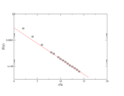
Figure 1: The effective range $F(r)$ as a function of $r/a$ on the $16^{3}\,32$ lattice at $\beta=8.45$ for $\rho=1.4$, together with an exponential fit. The fit gave $\mu=1.11(1)$.

The mass parameter $\rho$ influences the simulation in two ways. First, it affects the locality properties Hernandez of the Neuberger-Dirac operator. In Fig. 1 we show the effective range of $D_{N}$,

$$F(r)=\left\langle\left\langle\max_{x}|D_{N}(x,y)|\,\Big{|}_{||x-y||=r}\right\rangle_{y}\,\right\rangle_{U}\,,$$ (14)

with respect to the Euclidean distance

$$||x||=\left(\sum_{\mu=1}^{4}x_{\mu}^{2}\right)^{\frac{1}{2}}\,.$$ (15)

Figure 2: Condition number and $\mu$ on the $16^{3}\,32$ lattice at $\beta=8.45$ for $\rho=1.2$, $1.3$, $1.4$, $1.5$ and $1.6$, from left to right.

Asymptotically, $F(r)\propto\exp{-\mu r/a}$, where $\mu$ depends (among others) on $\rho$. (Numerically, $\mu\approx 2\,\nu$, where $\nu$ refers to the taxi driver distance Hernandez .) We want $\mu$ to be as large as possible, in particular $2\mu\gg m_{H}a$ ($3\mu\gg m_{H}a$) for mesons (baryons). Secondly, the condition number of $P_{\perp}^{N}H_{W}^{2}(\rho)$, $\kappa=\mu^{2}_{\rm max}/\mu^{2}_{N+1}$, depends on $\rho$ as well. In Fig. 2 we show the $\rho$ dependence of $\mu$ and $\kappa$ on the $16^{3}\,32$ lattice at $\beta=8.45$ for $N=10$. Test runs show, however, that $\kappa$ does not decrease significantly anymore if we increase $N$ further. We have chosen $\rho=1.4$, which is a trade-off between a small condition number $\kappa$ and a large value of $\mu$. At this value of $\rho$ we find $\mu=1.11(1)$, which is consistent with the results obtained in Hernandez from the Wilson gauge action.

The simulations are performed at the following quark masses:

$$\beta$$

0.0168 0.0280 0.0420 0.0560 0.0840 0.1400 0.1960

0.0280 0.0560 0.0980 0.1400

0.0112 0.0196 0.0280 0.0560 0.0980 0.1400

(16)

This covers the range of pseudoscalar masses $250\lesssim m_{PS}\lesssim 900\,\mbox{MeV}$ as we shall see. The lowest quark mass was chosen such that $m_{PS}L\gtrsim 3$ ($L$ being the spatial extent of the lattice). On all our lattices we have $L\gg 1/(2f_{\pi})$.

$O(a)$ improvement, both for masses and on- and off-shell operator matrix elements, is achieved by simply replacing $D$ by QCDSF1

$$D^{\rm imp}\equiv\left(1-\frac{am}{2\rho}\right)\,D\,\left(1-\frac{a}{2\rho}D\right)^{-1}$$ (17)

in the calculation of the quark propagator. Apart from the multiplicative mass term, this amounts to subtracting the contact term from the propagator. In the following we shall always use the improved propagator, without mentioning it explicitly. The eigenvalues of $D_{N}$ lie on a circle of radius $\rho/a$ around $(\rho/a,0)$ in the complex plane, while the eigenvalues of the improved operator $\displaystyle D_{N}^{\rm imp}=D_{N}\left(1-\frac{a}{2\rho}D_{N}\right)^{-1}$ lie on the imaginary axis.

IV Hadron Masses and Pseudoscalar Decay Constant

Let us now turn to the calculation of hadron masses and the pseudoscalar decay constant. Before we can compare our results with the real world, we have to set the scale. We will use the pion decay constant to do so, for reasons which will become clear later. The pion decay constant derives from the axial vector current, which has to be renormalized in the process.

IV.1 Calculational Details

The coefficients $c_{1}$, $c_{2}$ of the gauge field action are Gattringer $c_{1}=-0.169805$, $c_{2}=-0.0163414$ at $\beta=8.0$ and $c_{1}=-0.154846$, $c_{2}=-0.0134070$ at $\beta=8.45$. For the gauge field update we use a heat bath algorithm, which we repeat 1000 times to generate a new configuration.

The inversion of the overlap operator $D$ is done by solving the system of equations

$$Ax=y\,,$$ (18)

where $A=D^{\dagger}D$ and $y$ is the relevant source vector. We use the conjugate gradient algorithm for that. The speed of convergence depends on the condition number of the operator $A$, $\kappa(A)=\nu_{\rm max}/\nu_{\rm min}$, where $\nu_{\rm max}$ ($\nu_{\rm min}$) is the largest (lowest) eigenvalue of $A$. For reasonable values of the quark mass we have $\kappa(A)\propto 1/m_{q}^{2}$. Thus, the number of iterations, $n_{D}$, needed to achieve a certain accuracy will grow like $n_{D}\propto 1/m_{q}$ as the quark mass is decreased.

The convergence of the algorithm can be accelerated by a preconditioning method. Instead of (18) we solve the equivalent system of equations

$$ACx=Cy\equiv\tilde{A}x\,,$$ (19)

where $C$ is a nonsingular matrix, which we choose such that $\kappa(\tilde{A})\ll\kappa(A)$. Our choice is

$$C=1+\sum_{i=1}^{n}\left(\frac{1}{\nu_{i}}-1\right)v_{i}^{\phantom{\dagger}}v_{i}^{\dagger}\,,$$ (20)

where $v_{i}$ ($\nu_{i}$) are the normalized eigenvectors (eigenvalues) of $A$. The condition number of the operator $\tilde{A}$ is by a factor $\nu_{n+1}/\nu_{1}$ smaller than the condition number of the operator $A$, and the number of iterations in the conjugate gradient algorithm reduces to $n_{D}\propto 1/\sqrt{\nu_{n+1}+m^{2}_{q}}$, which depends only weakly on the quark mass $m_{q}$. We have chosen $n=80$, and the inversion was stopped when a relative accuracy of $10^{-7}$ was reached.

In the calculation of meson and baryon correlation functions we use smeared sources to improve the overlap with the ground state, while the sinks are taken to be either smeared or local. We use Jacobi smearing for source and sink QCDSF5 . To set the size of the source, we have chosen $\kappa_{s}=0.21$ for the smearing hopping parameter and employed $N_{s}=50$ smearing steps.

To further improve the signal of the correlation functions, we have deployed low-mode averaging lma in some cases by breaking the quark propagator into two pieces,

$$\sum_{i=1}^{n_{\ell}}\frac{\psi_{i}(x)\psi_{i}^{\dagger}(y)}{\lambda_{i}^{\rm imp}+m_{q}}\,,$$ (21)

where the sum extends over the eigenmodes of the $n_{\ell}$ lowest eigenvalues of $D_{N}^{\rm imp}$, and the remainder. The contribution from the low-lying modes (21) is averaged over all positions of the quark sources. As the largest contribution to the correlation functions comes from the lower modes, we may expect a significant improvement in the regime of small quark masses. We have chosen $n_{\ell}=40$, mainly because of memory limitations.

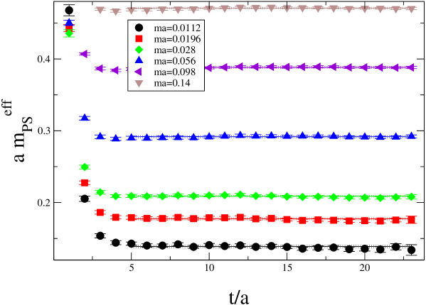
Figure 3: The effective pseudoscalar mass from the correlation function of the axial vector current $A_{4}$ on the $24^{3}\,48$ lattice at $\beta=8.45$, using smeared sources and local sinks.

IV.2 Lattice Results

The calculations are based on $900-1300$ gauge field configurations at the lowest four quark masses at $\beta=8.0$, and on $200-300$ configurations elsewhere. We consider hadrons only with all quarks having degenerate masses.

Pion Mass

To compute the pseudoscalar mass, $m_{PS}$, we looked at correlation functions of the pseudoscalar density $P=\bar{\psi}\gamma_{5}\psi$ and the time component of the axial vector current $A_{4}=\bar{\psi}\gamma_{4}\gamma_{5}\psi$. In Fig.3 we show the corresponding effective mass for our four lowest quark masses on the $24^{3}\,48$ lattice. Local sinks are found to give slightly smaller error bars than smeared sinks, so that we will restrict ourselves to this case. Both correlators give consistent results. We will use the results from the axial vector current correlator here, because it results in a wider plateau as the pseudoscalar correlator, in particular at the larger quark masses. We fit the correlator by the function $A\cosh\left(m_{PS}(t-T/2)\right)$, where $T$ is the temporal extent of the lattice, over the region of the plateau. The results of the fit are listed in Table 1.

$\beta$	$V$	$am_{q}$	$am_{PS}$	$am_{V}$	$am_{N}$	$af_{PS}$	$m_{PS}$ [MeV]
		0.0168	0.190(1)	0.643(5)	0.793(5)	0.075(1)	239(1)
		0.0280	0.235(1)	0.64935)	0.821(4)	0.076(1)	295(1)
		0.0420	0.281(1)	0.65923)	0.863(3)	0.078(1)	353(1)
$8.00$	$16^{3}\,32$	0.0560	0.321(1)	0.669(2)	0.890(3)	0.080(1)	403(1)
		0.0840	0.388(1)	0.695(3)	0.952(7)	0.082(1)	488(1)
		0.1400	0.502(1)	0.751(2)	1.074(7)	0.090(1)	631(1)
		0.1960	0.599(1)	0.815(1)	1.188(7)	0.097(1)	753(1)
		0.0280	0.212(3)	0.441(6)∗	0.595(6)∗	0.053(1)	396(8)
		0.0560	0.289(2)	0.482(4)∗	0.675(4)∗	0.058(1)	545(4)
$8.45$	$16^{3}\,32$
		0.0980	0.384(2)	0.537(4)	0.784(7)	0.064(1)	727(4)
		0.1400	0.467(2)	0.595(3)	0.886(6)	0.070(1)	883(4)
		0.0112	0.139(1)	0.429(6)∗	0.551(12)∗	0.051(1)	264(4)
		0.0196	0.177(1)	0.442(6)∗	0.572(11)∗	0.052(1)	336(2)
		0.0280	0.209(1)	0.452(3)∗	0.600(10)∗	0.054(1)	396(2)
$8.45$	$24^{3}\,48$
		0.0560	0.292(1)	0.481(3)	0.674(12)	0.058(1)	551(2)
		0.0980	0.388(1)	0.538(2)	0.788(11)	0.065(1)	731(2)
		0.1400	0.412(1)	0.597(1)	0.892(11)	0.071(1)	887(2)

Table 1: Hadron masses and pseudoscalar decay constant. The numbers marked by $\ast$ are obtained with low-mode averaging. To convert $m_{PS}$ to physical units, we have used the result in (28). The error on $m_{PS}$ in the last column is purely statistical.

Rho and Nucleon Mass

To compute the vector meson mass, $m_{V}$, we explored correlation functions of operators $V_{i}=\bar{\psi}\gamma_{i}\psi$ and $V^{4}_{i}=\bar{\psi}\gamma_{i}\gamma_{4}\psi$ ($i=1,2,3$). We found that the operator $V_{i}$, in combination

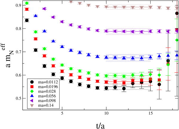
Figure 4: The effective nucleon mass on the $24^{3}\,48$ lattice at $\beta=8.45$, using smeared sources and local sinks. The horizontal lines indicate the fit interval as well as the value and error of the mass. The data points at the lowest three quark masses have been computed with low-mode averaging.

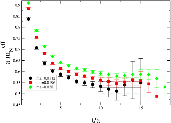
Figure 5: The same as the previous figure, but for the lowest three quark masses without using low-mode averaging.

with a local sink, gives the best signal.

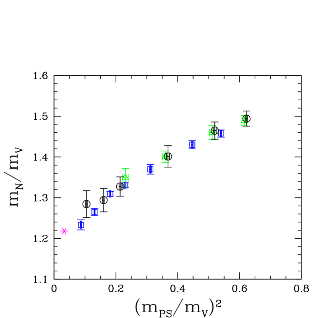
Figure 6: APE plot on the $24^{3}\,48$ lattice at $\beta=8.45$ ($\Circle$) and on the $16^{3}\,32$ lattices at $\beta=8.0$ ($\square$) and $\beta=8.45$ ($\vartriangle$).

For the calculation of the nucleon mass, $m_{N}$, we used $B_{\mu}=\varepsilon_{abc}\psi_{\mu}^{a}(\psi^{b}C\gamma_{5}\psi^{c})$ (where $C=\gamma_{4}\gamma_{2}$) as our basic operator, where we have replaced each spinor by $\psi\rightarrow\psi^{NR}=(1/2)(1+\gamma_{4})\psi$ QCDSF5 . These so-called nonrelativistic wave functions have a better overlap with the ground state than the ordinary, relativistic ones. In Fig. 4 we show the effective nucleon mass for all our six quark masses on the $24^{3}\,48$ lattice, where for the lowest three quark masses we have employed low-mode averaging. We find good to reasonable plateaus starting at $t/a\gtrsim 8$. In Fig. 5 we show, for comparison, the result obtained without low-mode averaging. In this case the situation is less favorable. The nucleon mass is obtained from a fit of the data by the correlation function $A\exp(-m_{N}t)+B\exp(-m_{N^{*}}(T-t))$, where $m_{N^{*}}$ is the mass of the backward moving baryon, over the region of the plateau.

The results for the rho and nucleon masses are listed in Table 1. Note that $am_{V}\ll 2\mu$ and $am_{N}\ll 3\mu$, respectively, are satisfied in all cases. In Fig. 6 we show an APE plot for our three lattices. At our smallest quark masses we have $m_{PS}/m_{V}\approx 0.3$. The APE plot shows no scaling violations outside the error bars and no finite size effects.

Pion decay constant

The physical pion decay constant is given by

$$\langle 0|\mathcal{A}_{4}|\pi\rangle=m_{\pi}f_{\pi}\,,$$ (22)

where $\mathcal{A}_{\mu}$ is the renormalized axial vector current, $\mathcal{A}_{\mu}=Z_{A}A_{\mu}$. Using the axial Ward identity

$$\partial_{\mu}\mathcal{A}_{\mu}=2m_{q}P\,,$$ (23)

where $P$ is the local pseudoscalar density, and considering the fact that $m_{q}P$ is a renormalization group invariant, we obtain

$$f_{\pi}=\frac{2m_{q}}{m^{2}_{\pi}}\langle 0|P|\pi\rangle\,.$$ (24)

On the lattice we consider the correlation function

$$\begin{split}\langle P^{s}(t)P^{s^{\prime}}(0)\rangle&=\frac{1}{2am_{PS}}\langle 0|P^{s}|PS\rangle\langle PS|P^{s^{\prime}}|0\rangle\,\left[\exp(-m_{PS}\,t)+\exp(-m_{PS}\,(T-t))\right]\\[3.99994pt] &\equiv A^{ss^{\prime}}\,\left[\exp(-m_{PS}\,t)+\exp(-m_{PS}\,(T-t))\right]\,,\end{split}$$ (25)

where the superscripts $s,s^{\prime}$ distinguish between local ($L$) and smeared ($S$) operators. From this we obtain

$$af_{PS}=am_{q}\left(\frac{2}{am_{\pi}}\right)^{3/2}\frac{A^{LS}}{\sqrt{A^{SS}}}\,.$$ (26)

We thus find $af_{PS}$ by computing $A^{LS}$ and $A^{SS}$. In Table 1 we give our results. In our notation the experimental value of $f_{\pi}$ is $92.4$ MeV.

Comparing our data on the $16^{3}\,32$ and $24^{3}\,48$ lattice at $\beta=8.45$ in Table 1 piece by piece, we also find no finite size effects down to the lowest common pseudoscalar mass.

IV.3 Setting the Scale: Pion Decay Constant

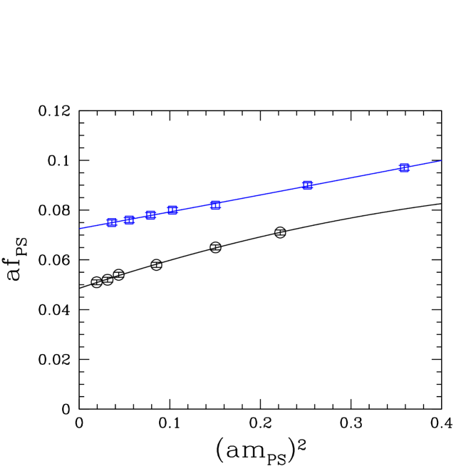
Figure 7: Chiral extrapolation of the pseudoscalar decay constant on the $24^{3}\,48$ lattice at $\beta=8.45$ ($\Circle$) and on the $16^{3}\,32$ lattice at $\beta=8.0$ ($\square$).

We will use the pseudoscalar decay constant to set the scale. The reason is that $f_{PS}$ is an analytic function in $m_{PS}^{2}$ for degenerate quark masses Pallante , in contrast to $m_{V}$ and $m_{N}$, which exhibit nonanalytic behavior. We thus expect that $f_{PS}$ extrapolates smoothly to the chiral limit. In quenched chiral perturbation theory Bernard ; Sharpe to NLO we have Pallante

$$f_{PS}=f_{0}\left(1+\alpha_{5}^{q}\frac{m_{PS}^{2}}{2(4\pi f_{0})^{2}}\right)+O(m_{PS}^{4})\,.$$ (27)

In Fig. 7 we show our data together with a quartic fit in the pseudoscalar mass. The lattice spacing is obtained from requiring $f_{PS}=f_{\pi}=92.4$ MeV at the physical pion mass. Using the $r_{0}/a$ values given in (13), we can convert the lattice spacing $a$ into the dimensionful scale parameter $r_{0}$. Altogether, we obtain

$$\beta$$ [fm] [MeV] [fm]

(28)

Note that $\alpha_{5}^{q}$, $f_{0}$ and $r_{0}$ come out independent of the lattice spacing within the error bars, which, once more, indicates good scaling properties of our action. The coefficient $\alpha_{5}^{q}$ turns out to be in agreement with the phenomenological value of $1.83$ ($L_{5}^{q}=0.00145$) reported in Bijnens .

IV.4 Comparison with Chiral Perturbation Theory

We shall now compare our results for the pseudoscalar, vector meson and nucleon mass with the predictions of chiral perturbation theory and attempt to extrapolate the lattice numbers to the chiral limit.

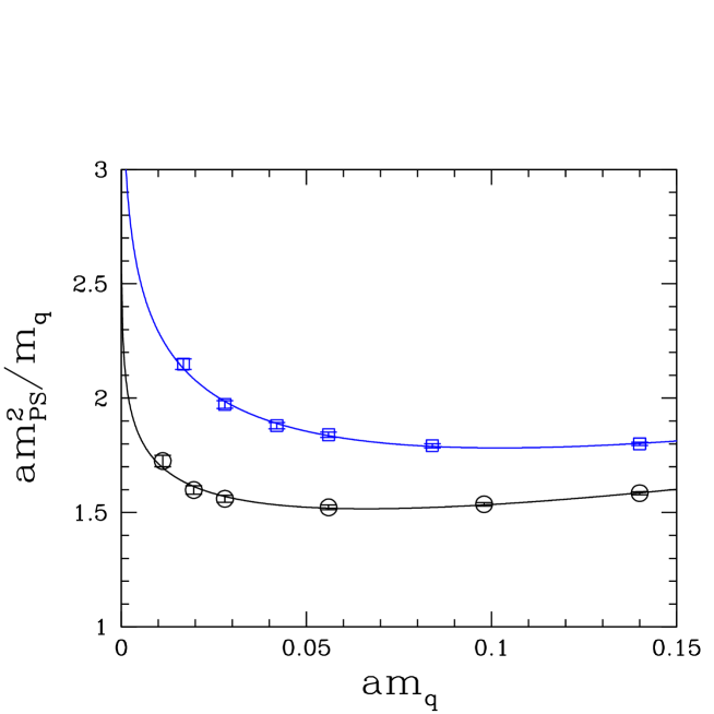
Figure 8: Chiral extrapolation of the pseudoscalar mass on the $24^{3}\,48$ lattice at $\beta=8.45$ ($\Circle$) and on the $16^{3}\,32$ lattice at $\beta=8.0$ ($\square$). The curves show the fits for $\alpha_{\Phi}^{q}=0$.

Pion Mass

We plot the pseudoscalar masses as a function of the quark mass in Fig. 8. Quenched chiral perturbation theory Bernard predicts in the infinite volume Pallante ; Sommer

$$\frac{m_{PS}^{2}}{m_{q}}=A\left\{1-\left(\delta-\frac{2}{3}\alpha_{\Phi}^{q}\,y\right)\big{(}\ln\,y+1\big{)}+\left[(2\alpha_{8}^{q}-\alpha_{5}^{q})-\frac{\alpha_{\Phi}^{q}}{3}\right]y\right\}+\cdots$$ (29)

with

$$y=\frac{Am_{q}}{\Lambda_{\chi}^{2}}$$ (30)

where $A=2\Sigma/f^{2}_{0}$, $\Sigma$ being the ‘bare quark condensate’, and $\Lambda_{\chi}$ denotes the scale at which the $\alpha_{i}$’s are being evaluated. The traditional value is $\Lambda_{\chi}=4\pi f_{0}$, which we will also adopt here. For the parameter $\delta$ chiral perturbation theory predicts Bernard ; Sharpe

$$\delta=\frac{\mu_{0}^{2}}{48\pi^{2}f_{\pi}^{2}}\,,$$ (31)

with $\mu_{0}^{2}\equiv m_{\eta^{\prime}}^{2}+m_{\eta}^{2}-2m_{K}^{2}=(870\,\mbox{MeV})^{2}$. This gives $\delta=0.183$. The parameters $f_{0}$ and $\alpha_{5}^{q}$ are known from our fit of $f_{PS}$ and are given in (28).

A much sought after quantity is the parameter $\delta$. Though unphysical, it would be a great success of the calculation, and of quenched chiral perturbation theory as well, if $\delta$ turned out to be in agreement with the predicted value. We shall try to determine $\delta$ directly from the data. Let us write

$$z=\frac{m_{PS}^{2}}{\Lambda_{\chi}^{2}}\,,\quad w=\frac{m_{PS}^{2}}{m_{q}}$$ (32)

and introduce the effective $\delta$ parameter

$$\delta_{\rm eff}^{-1}=1+\frac{\ln z^{\prime}\,w-\ln z\,w^{\prime}}{w-w^{\prime}}\,,$$ (33)

where $z,z^{\prime}$ and $w,w^{\prime}$, respectively, are adjacent data points. It is easy to see that

$$\lim_{m_{q}\rightarrow 0}\delta_{\rm eff}=\delta\,.$$ (34)

In Fig. 9 we show $\delta_{\rm eff}$ as a function of the quark mass. In the case of our high statistics run on the $16^{3}\,32$ lattice at $\beta=8.0$ we are able to extrapolate $\delta_{\rm eff}$ to the chiral limit. We obtain $\delta=0.18(4)$, in agreement with the prediction of quenched chiral perturbation theory. On the $24^{3}\,48$ lattice at $\beta=8.45$ our current statistics does not allow such an extrapolation. But the data for $\delta_{\rm eff}$ are not inconsistent with the predicted value of $\delta$.

The Witten-Veneziano formula WV relates $\mu_{0}^{2}$ to the topological susceptibility

$$\chi_{t}=\frac{\langle Q^{2}\rangle}{V}\,,$$ (35)

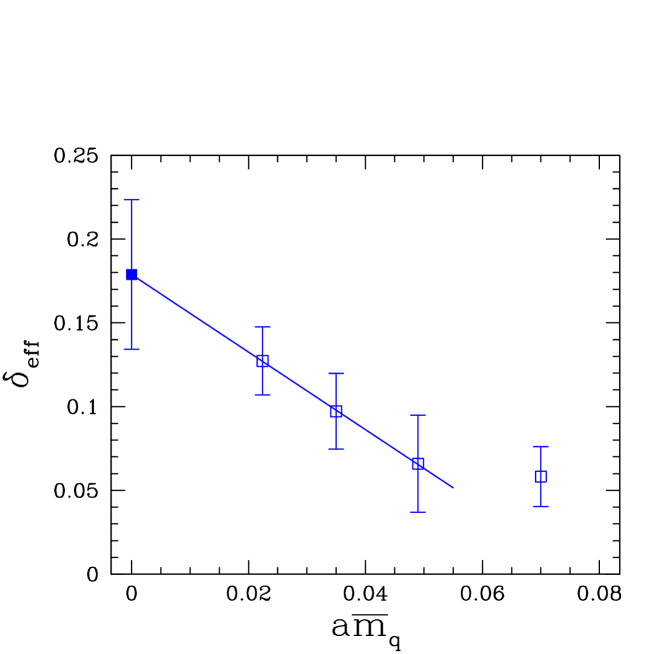
Figure 9: The parameter $\delta_{\rm eff}$ on the $16^{3}\,32$ lattice at $\beta=8.0$ together with a linear fit (top) and on the $24^{3}\,48$ lattice at $\beta=8.45$ (bottom), as a function of the average quark mass $\bar{m}_{q}=(m_{q}+m_{q}^{\prime})/2$.

where $Q$ is the topological charge and $V$ the lattice volume. The result for $\delta$ is

$$\delta=\frac{1}{8\pi^{2}f_{\pi}^{4}}\,\chi_{t}\,,$$ (36)

which suggests that the pseudoscalar mass depends on the topological charge $|Q|$. This turns out to be indeed the case. In Fig. 10 we show the pseudoscalar mass for various charge sectors, where the charge $Q$ is given by the index $\nu$ of $D_{N}$. We observe a strong increase of $\delta$ with increasing $|Q|$, and contrary to the findings in Brower , we do not expect the effect to go away in the limit $V\rightarrow\infty$, $\chi_{t}$ fixed. It would be interesting to search other quantities for a $|Q|$-dependence as well.

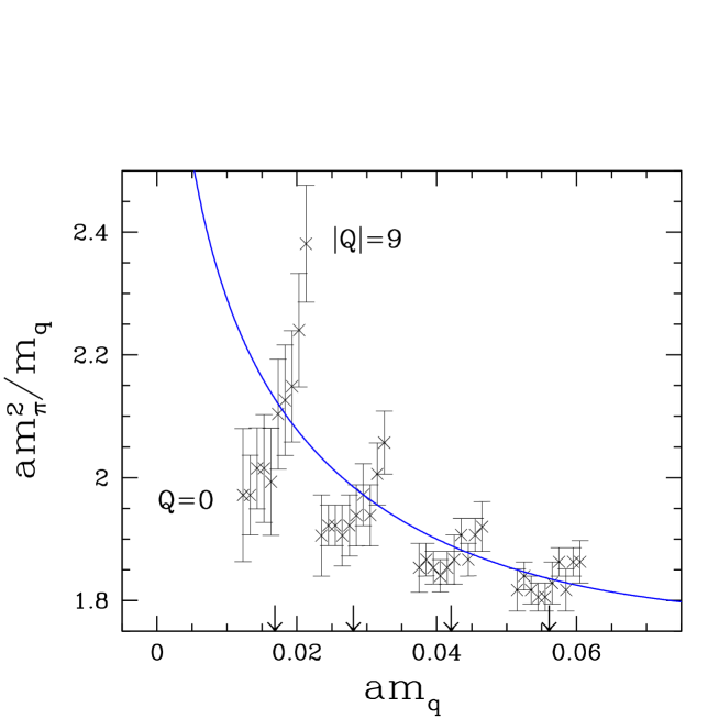
Figure 10: The pseudoscalar mass on the $16^{3}\,32$ lattice at $\beta=8.0$ for $|Q|=0,\cdots,9$, from left to right. The data have been displaced horizontally. The true quark masses are indicated by the arrow at the bottom rim of the figure. The curve is from Fig. 8.

Let us now turn to the fit of (29) to the data. Knowing $f_{0}$ and $\alpha_{5}^{q}$, this leaves us with four free parameters. Because our data do not allow an uncorrelated fit of all four parameters, we have to make a choice and fix one of them. We consider two cases. In the first case we fix $\alpha_{\Phi}$ at $0$, while in the second case we fix $\delta$ at its theoretical value of $0.183$. The two fits give

$$\beta$$

(37)

where we have omitted the heaviest mass point at $\beta=8.00$. The numbers shown in italics are the numbers that we fixed. It is not expected that $A$ scales. Assuming $\delta=0.183$ and taking $f_{0}$ from (28), we obtain $a^{3}\Sigma=0.0039(1)$ at $\beta=8.0$ and $a^{3}\Sigma=0.00138(5)$ at $\beta=8.45$, respectively. We shall return to $\Sigma$ and the fit function (29) when we compute the renormalized chiral condensate and quark masses. Combining the results on both lattices, we obtain $a_{8}^{q}=1.5(4)$ for $\delta=0.183$. This is to be compared with Sommer $a_{8}=0.8(4)$ in full QCD. In Fig. 8 we compare the fits with the data.

Rho Mass

In Fig. 11 we plot the vector meson masses as a function of the pseudoscalar mass, where we have used the results of (28) to convert the lattice numbers to physical values. Quenched chiral perturbation theory predicts Booth

$$m_{V}=C_{0}^{V}+C_{1/2}^{V}\,m_{PS}+C_{1}^{V}\,m_{PS}^{2}+C_{3/2}^{V}\,m_{PS}^{3}+\cdots\,,$$ (38)

where $m_{PS}$ is the lattice pseudoscalar mass as described by (29). The coefficient $C_{1/2}^{V}$ is expected to be negative, so that the chiral limit is approached from below. Our data show no indication of a cubic term, and so we shall drop that. A quadratic fit in the pseudoscalar mass gives

$$\beta$$

(39)

Our high statistics run at $\beta=8.0$ gives indeed a negative value for $C_{1/2}$, but perhaps of lower magnitude than expected Booth , while at $\beta=8.45$ our statistics is not high enough to make any statement. The fits are shown in Fig. 11. One might think that at the lighter quark masses one is seeing the lowest two-pion state instead of the rho. In Fig. 11 we also show the energy of two pseudoscalar mesons at the lowest nonvanishing lattice momentum, $|p|=2\pi/(aL)$, assuming the lattice dispersion relation to hold. We see that the lowest two-pion energy lies well above the vector meson mass because of the finite size of our lattice.

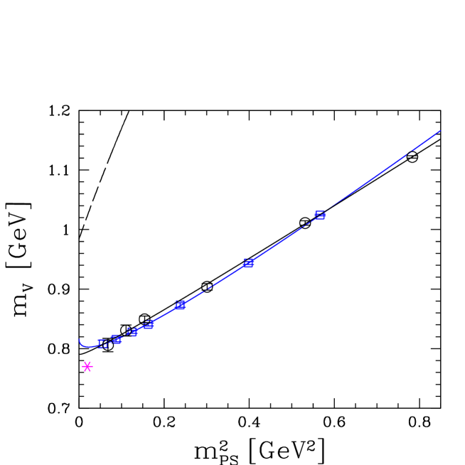
Figure 11: Chiral extrapolation of the vector meson mass on the $24^{3}\,48$ lattice at $\beta=8.45$ ($\Circle$) and on the $16^{3}\,32$ lattice at $\beta=8.0$ ($\square$), together with the experimental value ($\ast$). The solid curves show the fits. The dashed curve in the top left corner shows the energy of the state of two pseudoscalar mesons.

Nucleon Mass

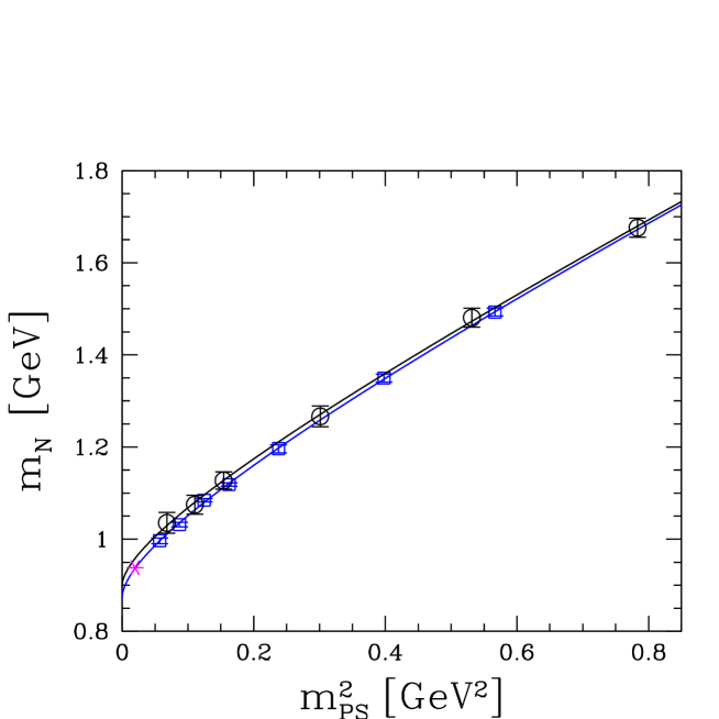
Figure 12: Chiral extrapolation of the nucleon mass on the $24^{3}\,48$ lattice at $\beta=8.45$ ($\Circle$) and on the $16^{3}\,32$ lattice at $\beta=8.0$ ($\square$), together with the experimental value ($\ast$). The curves show the fits.

We plot the nucleon masses as a function of the pseudoscalar mass in Fig. 12. Quenched chiral perturbation theory predicts Labrenz

$$m_{N}=C_{0}^{N}+C_{1/2}^{N}\,m_{PS}+C_{1}^{N}\,m_{PS}^{2}+C_{3/2}^{N}\,m_{PS}^{3}+\cdots\,,$$ (40)

where

$$C_{1/2}^{N}=-\frac{3}{2}\left(3F-D\right)^{2}\pi\delta\,.$$ (41)

Assuming the tree-level values $F=0.50$ and $D=0.76$, we expect $C_{1/2}^{N}=-2.58\,\delta$. For the theoretical value $\delta=0.183$ this would give $C_{1/2}^{N}=-0.47$. Of course, $F$ and $D$ may be different in the quenched theory. In the $N_{c}\rightarrow\infty$ limit, for example, $F/D=1/3$ giving $C_{1/2}^{N}=0$. Again, our data show no indication of a cubic term, and we shall drop that here as well. A quadratic fit in the pseudoscalar mass gives

$$\beta$$

(42)

At $\beta=8.0$ we find some evidence for nonanalytic behavior, but with positive coefficient $C_{1/2}^{N}$. The fits are shown in Fig. 12.

Both, the vector meson and nucleon masses scale, within the error bars, with the inverse lattice spacing set by the pion decay constant $f_{\pi}$.

V Nonperturbative Renormalization

We shall now turn to the determination of the renormalization constants $Z_{S}$, $Z_{P}$ and $Z_{A}$ of the scalar and pseudoscalar density and the axial vector current, respectively, which we will need in order to compute the renormalized quark mass. We shall employ the $RI^{\prime}-MOM$ scheme Martinelli . Our implementation of this method is described in QCDSF7 .

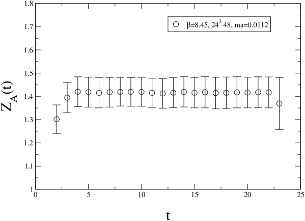
Figure 13: The renormalization constant $Z_{A}$ on the $24^{3}\,48$ lattice at $\beta=8.45$ at the smallest quark mass.

We consider amputated Green functions, or vertex functions, $\Gamma_{\mathcal{O}}$, with operator insertion $\mathcal{O}=S,\,P$ and $A_{4}$ in the Landau gauge. Defining renormalized vertex functions by

$$\Gamma_{\mathcal{O}}^{R}(p)=Z_{q}(\mu)^{-1}Z_{\mathcal{O}}(\mu)\,\Gamma_{\mathcal{O}}(p)\,,$$ (43)

where $\mu$ is the renormalization scale, we fix the renormalization constants by imposing the renormalization condition

$$\frac{1}{12}\,{\rm Tr}\left[\Gamma_{\mathcal{O}}^{R}(p)\,\Gamma_{\mathcal{O},\,{\rm Born}}^{-1}\right]\,\Big{|}_{p^{2}=\mu^{2}}=1\,.$$ (44)

That is, we compute the renormalization constants from

$$Z_{q}(\mu)^{-1}Z_{\mathcal{O}}(\mu)\,\frac{1}{12}\,{\rm Tr}\left[\Gamma_{\mathcal{O}}(p)\,\Gamma_{\mathcal{O},\,{\rm Born}}^{-1}\right]\Big{|}_{p^{2}=\mu^{2}}\equiv Z_{q}(\mu)^{-1}Z_{\mathcal{O}}(\mu)\,\Lambda_{\mathcal{O}}(p)\Big{|}_{p^{2}=\mu^{2}}=1$$ (45)

with $\Gamma_{S,\,{\rm Born}}=1$, $\Gamma_{P,\,{\rm Born}}=\gamma_{5}$ and $\Gamma_{A,\,{\rm Born}}=\gamma_{4}\gamma_{5}$.

Figure 14: Chiral extrapolation of $Z_{A}$ on the $24^{3}\,48$ lattice at $\beta=8.45$, together with its value in the chiral limit ($\CIRCLE$) .

The renormalization constant of the axial vector current can be directly determined from the axial Ward identity

$$Z_{A}=\frac{2m_{q}\left<P\left(t\right)P\left(0\right)\right>}{\left<\partial_{4}A_{4}\left(t\right)P\left(0\right)\right>}\,.$$ (46)

The wave function renormalization constant $Z_{q}$ can thus be obtained from $\Lambda_{A}$ and $Z_{A}$,

$$Z_{q}(\mu)=Z_{A}\,\Lambda_{A}\,.$$ (47)

In Fig. 13 we plot $Z_{A}$. We find that the r.h.s. of (46) is independent of $t$, except for the points close to source and sink, as expected. We extrapolate $Z_{A}$ linearly in $am_{q}$ to the chiral limit, as shown in Fig. 14. The final result is

$$\beta$$

1.59(1)

1.42(2)

1.42(1)

(48)

The corresponding fully tadpole improved (FTI) perturbative numbers QCDSF8 are $Z_{A}=1.358$ at $\beta=8.0$ and $Z_{A}=1.303$ at $\beta=8.45$. They lie $15\%-8\%$ below their nonperturbative values.

Let us now turn to the calculation of $\Lambda_{S}(p)$, $\Lambda_{P}(p)$ and $\Lambda_{A}(p)$. We denote the expressions at finite $m_{q}$ by $\Lambda(p,m_{q})$. Strictly speaking, $\Lambda_{S}(p,m_{q})$ and $\Lambda_{P}(p,m_{q})$ cannot be extrapolated to the chiral limit. Due to the zero modes, both $\Lambda_{S}(p,m_{q})$ and $\Lambda_{P}(p,m_{q})$ diverge $\propto 1/m_{q}^{2}$. This is an artefact of the quenched approximation. On top of that, $\Lambda_{P}(p,m_{q})$ receives a contribution $\propto\Sigma/(m_{q}p^{2})$. This term is due to spontaneous chiral symmetry breaking Pagels ; QCDSF7 . We thus expect the following dependence on the quark mass:

$$\Lambda_{S}(p,m_{q}) = \frac{C_{1}^{S}(p)}{(am_{q})^{2}}+C_{3}^{S}(p)+C_{4}^{S}(p)\,am_{q}\,,$$ (49)

$$\Lambda_{P}(p,m_{q}) = \frac{C_{1}^{P}(p)}{(am_{q})^{2}}+\frac{C_{2}^{P}(p)}{am_{q}}+C_{3}^{P}(p)+C_{4}^{P}(p)\,am_{q}\,,$$ (50)

$$\Lambda_{A}(p,m_{q}) = C_{3}^{A}(p)+C_{4}^{A}(p)\,am_{q}\,,$$ (51)

neglecting terms of $O(m_{q}^{2})$. This behavior is indeed shown by the data. In Fig. 15 we plot $\Lambda_{S}(p,m_{q})$, $\Lambda_{P}(p,m_{q})$ and $\Lambda_{A}(p,m_{q})$ for three different momenta, together with a fit of (49), (50) and (51) to the data. We identify $\Lambda_{S}(p)$, $\Lambda_{P}(p)$ and $\Lambda_{A}(p)$ with $c_{3}^{S}(p)$, $c_{3}^{P}(p)$ and $c_{3}^{A}(p)$, respectively, from which we derive

$$Z_{S}(\mu)=\frac{\Lambda_{A}(\mu)}{\Lambda_{S}(\mu)}\,Z_{A}\,,\quad Z_{P}(\mu)=\frac{\Lambda_{A}(\mu)}{\Lambda_{P}(\mu)}\,Z_{A}\,.$$ (52)

We expect $Z_{S}(\mu)=Z_{P}(\mu)$ due to chiral symmetry. To test this relation, we plot the ratio $\Lambda_{S}/\Lambda_{P}$ in Fig. 16. We find good agreement between $Z_{S}$ and $Z_{P}$ for all momenta. In the following we shall make use of a combined fit of $\Lambda_{S}(p,m_{q})$ and $\Lambda_{P}(p,m_{q})$, in which we set $C_{3}^{S}(p)=C_{3}^{P}(p)$.

We are finally interested in $Z_{S}$ in the $\overline{MS}$ scheme at a given scale $\mu$. To convert our numbers from the $RI^{\prime}-MOM$ scheme, which we were working in so far, to the $\overline{MS}$ scheme, we proceed in two steps. In the first step we match to the scale invariant $RGI$ scheme,

$$Z_{S}^{RGI}=\Delta^{RI^{\prime}-MOM}(\mu)\,Z_{S}(\mu)\,,$$ (53)

and in the second step we evolve $Z_{S}^{RGI}$ to the targeted scale in the $\overline{MS}$ scheme,

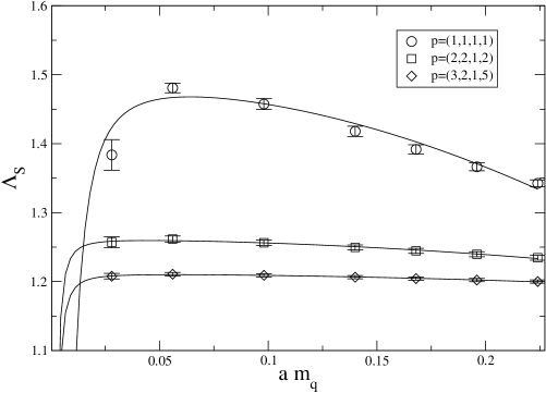
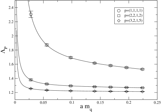
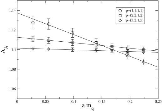
Figure 15: Chiral extrapolation of $\Lambda_{S}$ (top), $\Lambda_{P}$ (middle) and $\Lambda_{A}$ (bottom) on the $16^{3}\,32$ lattice at $\beta=8.45$ for some representative momenta $p=(n_{1},n_{2},n_{3},n_{4})$ in units of $2\pi/aL$ ($n_{1},n_{2},n_{3}$) and $\pi/aL$ ($n_{4}$).

$$Z_{S}^{\overline{MS}}(\mu)=\Delta^{\overline{MS}}(\mu)^{-1}\,Z_{S}^{RGI}\,.$$ (54)

The matching coefficients $\Delta^{RI^{\prime}-MOM}(\mu)$ and $\Delta^{\overline{MS}}(\mu)$ are known perturbatively to four loops 4loop . In Fig. 17 we show $Z_{S}^{RGI}$. The result is not quite independent of the scale parameter $\mu$ as it should, but shows a linear decrease in $\mu^{2}$ for $\mu\gtrsim 2\,\mbox{GeV}$. We attribute this behavior to lattice artefacts of $O(a^{2}\mu^{2})$. Indeed, the slope of $Z_{S}^{RGI}$ at our two different $\beta$ values scales like $a^{2}$ to a good approximation. We thus fit the lattice result by

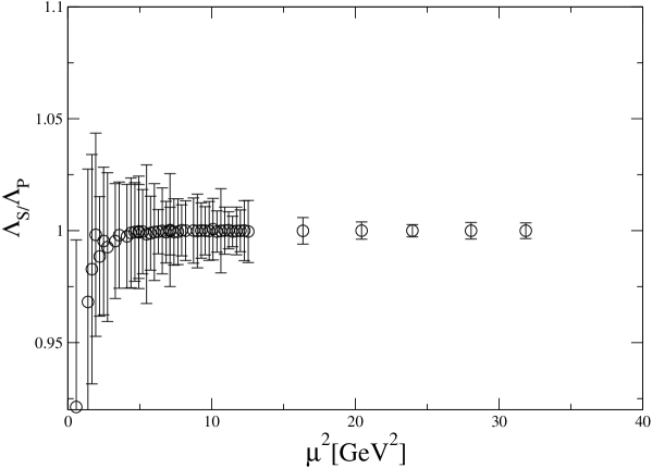
Figure 16: The ratio $\Lambda_{S}(\mu)/\Lambda_{P}(\mu)$ as a function of $\mu$ on the $16^{3}\,32$ lattice at $\beta=8.45$.

$$Z_{S}^{RGI,LAT}=C_{0}+C_{1}(a\mu)^{2}$$ (55)

and identify the physical value of $Z_{S}^{RGI}$ with $C_{0}$. This finally gives

$$\beta$$

1.18(2)

1.02(1)

(56)

The four-loop value for $\Delta_{S}^{\overline{MS}}(\mu)$ has been given in QCDSF9 . At $\mu=2\,\mbox{GeV}$ it is $\Delta_{S}^{\overline{MS}}(2\,\mbox{GeV})=0.721(10)$. The error is a reflection of the error of $\Lambda^{\overline{MS}}$. The nonperturbative result at $\beta=8.45$ is in good agreement with $Z_{S}^{FTI,RGI}$ from QCDSF8 .

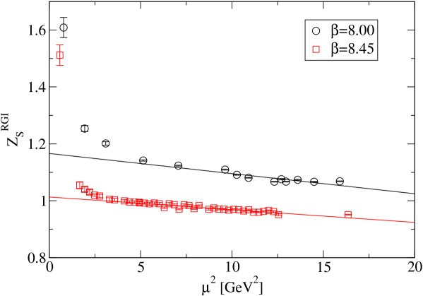
Figure 17: The scale invariant renormalization constant $Z_{S}^{RGI}$ on the $16^{3}\,32$ lattice at $\beta=8.0$ ($\Circle$) and $\beta=8.45$ ($\square$).

VI Chiral Condensate and Quark Masses

Having determined the renormalization constant of the scalar density, we may now compute the renormalized chiral condensate and light and strange quark masses.

Let us first consider the chiral condensate $\langle\bar{\psi}\psi\rangle$. Strictly speaking, $\langle\bar{\psi}\psi\rangle$ is not defined in the quenched theory due to the presence of a logarithmic singularity in the chiral limit. Nevertheless, we may identify $-\langle\bar{\psi}\psi\rangle$ with $\Sigma$ and assume that $\Sigma$ renormalizes like (the finite part of) the scalar density. In the $\overline{MS}$ scheme at $\mu=2\,\mbox{GeV}$ we then have

$$\langle\bar{\psi}\psi\rangle^{\overline{MS}}(2\,\mbox{GeV})=-Z_{S}^{\overline{MS}}(2\,\mbox{GeV})\,\Sigma\,.$$ (57)

Taking $\Sigma$ from our second fit in (37), where we have fixed $\delta$ to its theoretical value $0.183$, this leads to

$$\beta$$

(58)

The lower number at the larger $\beta$ value is in reasonable agreement with phenomenology and other quenched lattice calculations chicon . A better way to determine $\Sigma$ is by means of the spectral density Osborn ; Damgaard , which we will address in a separate publication Streuer .

Let us now turn to the evaluation of the quark masses. We shall assume (29) with $\alpha_{\Phi}^{q}=0$ as the basic functional form for the relation between the quark masses and the pseudoscalar mass:

$$m_{PS}^{2}=Xm_{q}+Ym_{q}\ln m_{q}+Zm_{q}^{2}\,.$$ (59)

For nondegenerate quark masses, $m_{q}^{a}$ and $m_{q}^{b}$, chiral perturbation theory gives the result

$$\begin{split}\left(m_{PS}^{ab}\right)^{2}&=X\left(\frac{m_{q}^{a}+m_{q}^{b}}{2}\right)+Y\left(\frac{m_{q}^{a}+m_{q}^{b}}{2}\right)\left(\frac{m_{q}^{a}\ln m_{q}^{a}-m_{q}^{b}\ln m_{q}^{b}}{m_{q}^{a}-m_{q}^{b}}-1\right)\\ &+\,Z\left(\frac{m_{q}^{a}+m_{q}^{b}}{2}\right)^{2}\end{split}$$ (60)

with no new parameter. In fact, (60) reduces exactly to (59) in the limit $m_{q}^{a}\rightarrow m_{q}^{b}$. We fit (59) to our data to determine the coefficients $X$, $Y$ and $Z$. The light quark mass, $m_{\ell}=(m_{u}+m_{d})/2$, is then found from

$$m_{\pi^{+}}^{2}=Xm_{\ell}+Ym_{\ell}\ln m_{\ell}+Zm_{\ell}^{2}\,,$$ (61)

while we compute the strange quark mass from

$$\begin{split}\frac{m_{K^{+}}^{2}+m_{K^{0}}^{2}}{2}&=X\left(\frac{m_{\ell}+m_{s}}{2}\right)+Y\left(\frac{m_{\ell}+m_{s}}{2}\right)\left(\frac{m_{\ell}\ln m_{\ell}-m_{s}\ln m_{s}}{m_{\ell}-m_{s}}-1\right)\\ &+\;Z\left(\frac{m_{\ell}+m_{s}}{2}\right)^{2}\,.\end{split}$$ (62)

The result is

$$\beta$$ [MeV] [MeV]

(63)

The renormalized quark masses are given by

$$m_{q}^{R}=Z_{m}\,m_{q}\,,$$ (64)

where $Z_{m}=1/Z_{S}$. Combining the bare quark masses in (63) with the results for $Z_{S}$ in (56) and below, we obtain in the $\overline{MS}$ scheme at $\mu=2\,\mbox{GeV}$

$$\beta$$ [MeV] [MeV]

(65)

These results are in good agreement with other nonperturbative calculations of the quark masses in the quenched approximation Rebbi ; Liu ; Garden ; QCDSF9 .

VII Conclusions

The extrapolation to the chiral limit has been a major challenge in lattice QCD. We have shown that with using overlap fermions it is possible to progress to small quark masses. Here we have simulated pion masses down to $m_{\pi}\approx 250$ MeV on both of our lattices. We have made an attempt to compute the low-energy constants of quenched chiral perturbation theory, with some success. Our results turn out to be consistent with the predicted and/or phenomenological values. To fully exploit the potential of overlap fermions at small quark masses, one will, however, need a statistics of several thousand independent gauge field configurations.

The pion mass was found to depend on the topological charge $|Q|$ at small quark masses. No such behavior was found for the pseudoscalar decay constant, but a similar effect is expected to show up in the chiral condensate Osborn .

Overlap fermions, in combination with the Lüscher-Weisz gauge field action, show good scaling properties already at lattice spacing $a\approx 0.15$ fm, owing to the fact that they are automatically $O(a)$ improved, on-shell and off-shell. This helps to reduce the large numerical overhead in the algorithm.

The calculations performed in this paper test many of the ingredients needed for a simulation of full QCD, and thus provide a lesson for future applications.

References

- (1) H. Neuberger, Phys. Lett. B417 (1998) 141; ibid. B427 (19998) 353.
- (2) M. Lüscher, Phys. Lett. B428 (1998) 342.
- (3) S. Capitani, M. Göckeler, R. Horsley, P. E. L. Rakow and G. Schierholz, Phys. Lett. B468 (1999) 150.
- (4) L. Giusti, C. Hoelbling and C. Rebbi, Phys. Rev. D64 (2001) 114508 [Erratum ibid. D65 (2002) 079903]; N. Garron, L. Giusti, C. Hoelbling, L. Lellouch and C. Rebbi, Phys. Rev. Lett. 92 (2004) 042001; F. Berruto, N. Garron, C. Hoelbling, J. Howard, L. Lellouch, S. Necco, C. Rebbi and N. Shoresh, Nucl. Phys. Proc. Suppl. 140 (2005) 264.
- (5) S. J. Dong, F. X. Lee, K. F. Liu and J. B. Zhang, Phys. Rev. Lett. 85 (2000) 5051; S. J. Dong, T. Draper, I. Horvath, F. X. Lee, K. F. Liu and J. B. Zhang, Phys. Rev. D65 (2002) 054507; F. X. Lee, S. J. Dong, T. Draper, I. Horvath, K. F. Liu, N. Mathur and J. B. Zhang, Nucl. Phys. Proc. Suppl. 119 (2003) 296; N. Mathur, F. X. Lee, A. Alexandru, C. Bennhold, Y. Chen, S.J. Dong, T. Draper, I. Horvath, K. F. Liu, S. Tamhankar and J. B. Zhang, Phys. Rev. D 70 (2004) 074508.
- (6) D. Galletly, M. Gürtler, R. Horsley, B. Joó, A. D. Kennedy, H. Perlt, B. J. Pendleton, P. E. L. Rakow, G. Schierholz, A. Schiller and T. Streuer, Nucl. Phys. Proc. Suppl. 129 (2004) 453.
- (7) W. Bietenholz, T. Chiarappa, K. Jansen, K. I. Nagai and S. Shcheredin, JHEP 0402 (2004) 023.
- (8) P. Hernandez, K. Jansen and M. Lüscher, Nucl. Phys. B552 (1999) 363.
- (9) G. Colangelo, Nucl. Phys. Proc. Suppl. 140 (2005) 120.
- (10) D. Galletly, M. Gürtler, R. Horsley, K. Koller, V. Linke, P. E. L. Rakow, C. J. Roberts, G. Schierholz and T. Streuer, PoS LAT2005 (2005) 363 [arXiv:hep-lat/0510050].
- (11) M. Gürtler, R. Horsley, V. Linke, H. Perlt, P. E. L. Rakow, G. Schierholz, A. Schiller and T. Streuer, Nucl. Phys. Proc. Suppl. 140 (2005) 707.
- (12) E. M. Ilgenfritz, K. Koller, Y. Koma, G. Schierholz, T. Streuer and V. Weinberg, arXiv:hep-lat/0512005.
- (13) V. Weinberg, E. M. Ilgenfritz, K. Koller, Y. Koma, G. Schierholz and T. Streuer, PoS LAT2005 (2005) 171 [arXiv:hep-lat/0510056].
- (14) L. Giusti, C. Hoelbling, M. Lüscher and H. Wittig, Comput. Phys. Commun. 153 (2003) 31.
- (15) M. Lüscher and P. Weisz, Commun. Math. Phys. 97 (1985) 59.
- (16) C. Gattringer, R. Hoffmann and S. Schaefer, Phys. Rev. D65 (2002) 094503.
- (17) K. Symanzik, Nucl. Phys. B226 (1983) 187.
- (18) M. Göckeler, R. Horsley, E.-M. Ilgenfritz, H. Perlt, P. Rakow, G. Schierholz and A. Schiller, Phys. Rev. D53 (1996) 2317.
- (19) T. DeGrand and S. Schaefer, Comput. Phys. Commun. 159 (2004) 185; L. Giusti, P. Hernandez, M. Laine, P. Weisz and H. Wittig, JHEP 0404 (2004) 013; A. O’Cais, K. J. Juge, M. J. Peardon, S. M. Ryan and J. I. Skullerud, Nucl. Phys. Proc. Suppl. 140 (2005) 844.
- (20) M. Göckeler, R. Horsley, H. Perlt, P. Rakow, G. Schierholz, A. Schiller and P. Stephenson, Phys. Rev. D57 (1998) 5562.
- (21) G. Colangelo and E. Pallante, Nucl. Phys. B520 (1998) 433.
- (22) C. W. Bernard and M. F. L. Golterman, Phys. Rev. D46 (1992) 853.
- (23) S. R. Sharpe, Phys. Rev. D46 (1992) 3146.
- (24) J. Gasser and H. Leutwyler, Nucl. Phys. B250 (1985) 465.
- (25) J. Bijnens, AIP Conf. Proc. 768 (2005) 153 [arXiv:hep-ph/0409068].
- (26) J. Heitger, R. Sommer and H. Wittig, Nucl. Phys. B588 (2000) 377.
- (27) E. Witten, Nucl. Phys. B156 (1979) 269; G. Veneziano, Nucl. Phys. B159 (1979) 213.
- (28) R. Brower, S. Chandrasekharan, J. W. Negele and U. J. Wiese, Phys. Lett. B560 (2003) 64.
- (29) M. Booth, G. Chiladze and A. F. Falk, Phys. Rev. D55 (1997) 3092.
- (30) J. N. Labrenz and S. R. Sharpe, Phys. Rev. D54 (1996) 4595.
- (31) G. Martinelli, C. Pittori, C. T. Sachrajda, M. Testa and A. Vladikas, Nucl. Phys. B445 (1995) 81.
- (32) M. Göckeler, R. Horsley, H. Oelrich, H. Perlt, D. Petters, P. E. L. Rakow, A. Schäfer, G. Schierholz and A. Schiller, Nucl. Phys. B544 (1999) 699.
- (33) R. Horsley, H. Perlt, P. E. L. Rakow, G. Schierholz and A. Schiller, Nucl. Phys. B693 (2004) 3 [Erratum ibid. B713 (2005) 601].
- (34) H. Pagels, Phys. Rev. D19 (1979) 3080.
- (35) K. G. Chetyrkin, Phys. Lett. B404 (1997) 161; J. A. M Vermaseren, S. A. Larin and T. van Ritbergen, Phys. Lett. B405 (1997) 327; K. G. Chetyrkin and A. Rétey, Nucl. Phys. B583 (2000) 3; see also M. Göckeler, R. Horsley, A. C. Irving, D. Pleiter, P. E. L. Rakow, G. Schierholz, H. Stüben and J. M. Zanotti, arXiv:hep-lat/0601004.
- (36) M. Göckeler, R. Horsley, H. Oelrich, D. Petters, D. Pleiter, P. E. L. Rakow, G. Schierholz, P. Stephenson M. Göckeler, Phys. Rev. D62 (2000) 054504.
- (37) J. C. Osborn, D. Toublan and J. J. M. Verbaarschot, Nucl. Phys. B540 (1999) 317.
- (38) P. H. Damgaard, Nucl. Phys. B608 (2001) 162.
- (39) L. Giusti, F. Rapuano, M. Talevi and A. Vladikas, Nucl. Phys. B538 (1999) 249; T. A. DeGrand, Phys. Rev. D64 (2001) 117501; P. Hernandez, K. Jansen, L. Lellouch and H. Wittig, JHEP 0107 (2001) 018; L. Giusti, C. Hoelbling and C. Rebbi, Phys. Rev. D64 (2001) 114508 [Erratum-ibid. D65 (2002) 079903]; T. Blum, P. Chen, N. Christ, C. Cristian, C. Dawson, G. Fleming, A. Kaehler, X. Liao, G. Liu, C. Malureanu, R. Mawhinney, S. Ohta, G. Siegert, A. Soni, C. Sui, P. Vranas, M. Wingate, L. Wu and Y. Zhestkov, Phys. Rev. D69 (2004) 074502; D. Becirevic and V. Lubicz, Phys. Lett. B600 (2004) 83; V. Gimenez, V. Lubicz, F. Mescia, V. Porretti and J. Reyes, Eur. Phys. J. C41 (2005) 535.
- (40) M. Gürtler et al., in preparation.
- (41) J. Garden, J. Heitger, R. Sommer and H. Wittig, Nucl. Phys. B571 (2000) 237.