Massive Domain Wall Fermions on Four-dimensional Anisotropic Lattices

Abstract

We formulate the massive domain wall fermions on anisotropic lattices. For the massive domain wall fermion, we find that the dispersion relation assumes the usual form in the low momentum region when the bare parameters are properly tuned. The quark self-energy and the quark field renormalization constants are calculated to one-loop in bare lattice perturbation theory. For light domain wall fermions, we verified that the chiral mode is stable against quantum fluctuations on anisotropic lattices. This calculation serves as a guidance for the tuning of the parameters in the quark action in future numerical simulations.

, , ,

1 Introduction

In recent years, considerable progress has been made in understanding chiral symmetry on the lattice. Domain wall fermions [1, 2] and the overlap fermions [3, 4, 5, 6] have emerged as two new candidates in the formulation of lattice fermions which have much better chiral properties than the conventional lattice Wilson or staggered fermions. Since chiral symmetry is so crucial to the theory of QCD, it is therefore desirable to use these new fermions if possible. However, due to their more expensive computational cost, this task has not been fully accomplished, particularly for the study of multi-hadron states and hadrons with massive quarks.

On the other hand, anisotropic lattices have been used to study heavy hadronic states and they proved to be extremely helpful in various applications. These include: glueball spectrum calculations [7, 8], charmonium spectrum calculations [9, 10], charmed meson and charmed baryon calculations [11, 12] and hadron-hadron scattering calculations [13, 14, 15, 16]. Many of these studies in fact involve light quarks and chiral symmetry plays an essential role. It is therefore more appropriate to study the light quarks using lattice fermions with better chiral properties. Using domain wall fermions with the physical four-dimensional lattice being isotropic, the heavy-light systems [17] and hadron-hadron scattering [18] have been studied. As we pointed out, anisotropic lattices can be very helpful in these studies. It is therefore desirable to study domain wall fermions with the four-dimensional physical lattice being anisotropic and this will be the major purpose of this paper. Major possible applications of the anisotropic domain wall fermion approach that we have in mind are the heavy-light hadrons, exotic hadrons with light quarks and hadron-hadron scattering processes where the objects being studied are heavy and chiral property is crucial.

In this paper, we study an explicit formulation of domain wall fermions on anisotropic four-dimensional lattices. We adopt the domain wall fermion action which is of Shamir type [2]. For the gauge action, we use the tadpole improved gauge actions [19, 7] which have been used in glueball calculations. Similar to the case of Wilson fermions on anisotropic lattices, domain wall fermion action on anisotropic lattices contains more parameters than its isotropic counterparts. Some of these parameters have to be tuned properly in order to exhibit a correct continuum limit. This problem is first analyzed in the case of free domain wall fermions on anisotropic lattices. We find that, in order to restore the normal relativistic dispersion relation for the quark, parameters of the fermion action has to be tuned accordingly. Then, we compute the quark propagator in lattice perturbation theory to one-loop. Quark field and quark mass renormalization constants are obtained for various values of the bare parameters. We also discuss the choice of the parameters which maintains good chiral symmetry. This perturbative calculation serves as a guidance for further non-perturbative Monte Carlo simulations which are currently under investigation [20]. Similar perturbative calculations have been performed in the case of isotropic lattice [21, 22]. The calculation in this paper is an extension to the anisotropic lattice.

This paper is organized as follows. In section 2, domain wall fermion action on anisotropic lattices is given. In section 3, the free domain wall fermion propagator on anisotropic lattices is derived. We also study the dispersion relation of the free domain wall fermion on anisotropic lattices. It turns out that even in the free case, hopping parameters of the fermion action have to be tuned properly, according to the value of the quark mass, so as to have the correct continuum limit for the quark. In section 4, the strategies for the calculations of fermion self-energy to one-loop are outlined. In section 5, numerical results for the one-loop calculation are presented for various bare parameters. The renormalization factors for the quark field and the current quark mass are given. We also discuss the renormalization of parameter $M_{5}$ within tadpole and mean-field approximation. This parameter has to be tuned to the right range in order to maintain chiral properties of the fermion. In section 6, we will conclude with some remarks and outlook. Dispersion relation of the free domain wall fermion is discussed in Appendix A. Some explicit formulae for the one-loop calculations are listed in Appendix B.

2 Lattice Action for Domain Wall Fermions on Anisotropic Lattices

The lattice gauge action used in this study is the tadpole improved action on anisotropic lattices: [19, 7]

$$S= - \beta\sum_{i>j}\left[{5\over 9}{TrP_{ij}\over\chi u^{4}_{s}}-{1\over 36}{TrR_{ij}\over\chi u^{6}_{s}}-{1\over 36}{TrR_{ji}\over\chi u^{6}_{s}}\right]$$ (1)

$$- \beta\sum_{i}\left[{4\over 9}{\chi TrP_{0i}\over u^{2}_{s}}-{1\over 36}{\chi TrR_{i0}\over u^{4}_{s}}\right]\;\;,$$

where $P_{0i}$ and $P_{ij}$ represents the usual temporal and spatial plaquette variable, respectively. $R_{ij}$ and $R_{i0}$ designates the $2\times 1$ spatial and temporal Wilson loops, where, in order to eliminate the spurious states, we have restricted the coupling of fields in the temporal direction to be within one lattice spacing. The parameter $u_{s}$, which is usually taken to be the fourth root of the average spatial plaquette value in the simulation, implements the tadpole improvement. Using this gauge action, glueball and hadron spectra have been studied within quenched approximation [19, 7, 8, 23, 24, 25, 26].

For the fermion action, we adopt Shamir type domain wall fermions [2]. The five-dimensional fermion and anti-fermion field is denoted as $\psi_{x,s}$ and $\bar{\psi}_{x,s}$, respectively. The fermion lattice action we studied is given by:

$$S_{f} = S^{\prime}_{f}+S_{m}\;,$$

$$S^{\prime}_{f} = -\sum_{x,s}(1+3\kappa_{s}+\kappa_{t}-M_{5})\bar{\psi}_{x,s}\psi_{x,s}$$

$$+ \sum_{x,s}\left[\bar{\psi}_{x,s}P_{R}\psi_{x,s+1}+\bar{\psi}_{x,s}P_{L}\psi_{x,s-1}\right]$$

$$+ {1\over 2}\sum_{x,s,\mu}\kappa_{\mu}\bar{\psi}_{x,s}\left[(1+\gamma_{\mu})U_{\mu}(x)\psi_{x+\hat{\mu},s}+(1-\gamma_{\mu})U^{\dagger}_{\mu}(x-\hat{\mu})\psi_{x-\hat{\mu},s}\right]\;,$$

$$S_{m} = -m\sum_{x}\left[\bar{\psi}_{x,0}P_{L}\psi_{x,L_{s}-1}+\bar{\psi}_{x,L_{s}-1}P_{R}\psi_{x,0}\right]\;,$$ (2)

We will also use the notation $\kappa_{0}=\kappa_{t}$, $\kappa_{i}=\kappa_{s}$. The left and right-handed projectors are: $P_{L/R}=(1\mp\gamma_{5})/2$. For definiteness, we take the extension in the fifth dimension to be $L_{s}$ and the coordinate of the fifth dimension is labelled such that $0\leq s\leq L_{s}-1$. Thus, our domain wall fermion action is characterized by four parameters: five-dimensional mass (wall height) parameter $M_{5}$, temporal hopping parameter $\kappa_{t}$, spatial hopping parameter $\kappa_{s}$ and current quark mass parameter $m$. .

3 Free Domain Wall Fermion Propagator on Anisotropic Lattices

In this section, we will briefly review the results for the free propagator of the domain wall fermions on anisotropic lattices. Free domain wall fermion propagator on an isotropic lattice has been discussed in the literature [2, 27, 21, 22]. Our notations follow those in [2, 22] and we have made modifications to the anisotropic lattice where necessary. We have also tried to keep all relevant mass terms (bare quark mass $m$ and the residual mass $m_{r}$) in the free domain wall propagator. This is useful in practice since we would like to apply the anisotropic lattice formalism to massive quarks (charm) and the extension in the fifth dimension is usually not very large in practical simulations.

3.1 The free propagator

After performing the four-dimensional Fourier transform, the free domain wall fermion matrix appearing in action (2) is given by:

$$D^{(0)}_{ss^{\prime}}(p) = \left[-b(p)+i{\tilde{p}\kern-4.49997pt/\kern 3.00003pt}\right]\delta_{ss^{\prime}}+\left[P_{R}\delta_{s+1,s^{\prime}}+P_{L}\delta_{s-1,s^{\prime}}\right]$$ (3)

$$- m\left(P_{L}\delta_{s,0}\delta_{s^{\prime},L_{s}-1}+P_{R}\delta_{s^{\prime},0}\delta_{s,L_{s}-1}\right)\;,$$

$$= \left[i{\tilde{p}\kern-4.49997pt/\kern 3.00003pt}+W^{+}(p)\right]P_{R}+\left[i{\tilde{p}\kern-4.49997pt/\kern 3.00003pt}+W^{-}(p)\right]P_{L}\;$$ (4)

where the function $b(p)$ and the notation ${\tilde{p}\kern-4.49997pt/\kern 3.00003pt}$ are defined as:

$$b(p) = 1-M_{5}+\sum_{\mu}\kappa_{\mu}(1-\cos p_{\mu})\;,$$

$${\tilde{p}\kern-4.49997pt/\kern 3.00003pt} = \sum_{\mu}\gamma_{\mu}\tilde{p}_{\mu}\;,\;\;\tilde{p}_{\mu}=\kappa_{\mu}\sin p_{\mu}\;.$$ (5)

The matrices $W^{\pm}(p)$ appearing in Eq. (4) are defined as:

$$[W^{+}(p)]^{\dagger}_{ss^{\prime}}\equiv\left[W^{-}(p)\right]_{ss^{\prime}}=-b(p)\delta_{ss^{\prime}}-m\delta_{L_{s}-1,s^{\prime}}\delta_{s,0}+\delta_{s-1,s^{\prime}}\;.$$ (6)

With this notation, one easily works out the second order operator $\Omega^{(0)}(p)$ which is defined as:

$$\Omega^{(0)}(p) \equiv D^{(0)}(p)\cdot\left[D^{(0)}(p)\right]^{\dagger}=\Omega^{(0)}_{L}(p)P_{L}+\Omega^{(0)}_{R}(p)P_{R}\;,$$ (7)

$$= \tilde{p}^{2}+W^{+}W^{-}P_{R}+W^{-}W^{+}P_{L}\;.$$

Note that the operators $\Omega^{(0)}_{L/R}(p)=\tilde{p}^{2}+W^{\mp}W^{\pm}$ have trivial Dirac structure and they are related to each other by:

$$\left[\Omega^{(0)}_{L}(p)\right]_{s,s^{\prime}}=\left[\Omega^{(0)}_{R}(p)\right]_{L_{s}-s-1,L_{s}-s^{\prime}-1}\;.$$ (8)

The matrices $W^{-}W^{+}$ and $W^{+}W^{-}$ are referred to as the mass matrices for the right and left-handed fermions, respectively. Free fermion propagator is then expressed in terms of the inverse of the second order operators as:

$$S_{F}(p) \equiv \left[D^{(0)}(p)]\right]^{-1}=\left[D^{(0)}(p)\right]^{\dagger}\cdot\left[\Omega^{(0)}(p)\right]^{-1}\;,$$ (9)

$$= \left[-i{\tilde{p}\kern-4.49997pt/\kern 3.00003pt}+W^{-}(p)\right]P_{R}G^{(0)}_{R}+\left[-i{\tilde{p}\kern-4.49997pt/\kern 3.00003pt}+W^{+}(p)\right]P_{L}G^{(0)}_{L}\;,$$

where we have used the notation:

$$G^{(0)}_{L/R}(p)=\left[\Omega^{(0)}_{L/R}(p)\right]^{-1}\;.$$ (10)

The explicit results for $G^{(0)}_{R}(p)$ and $G^{(0)}_{L}(p)$ are found to be:

$$\left[G^{(0)}_{R}(p)\right]_{s,s^{\prime}} = \left[G^{(\infty)}(p)\right]_{s,s^{\prime}}+A_{+}e^{-\alpha_{G}(s+s^{\prime})}+A_{-}e^{-\alpha_{G}(2L_{s}-2-s-s^{\prime})}$$

$$+ A_{m}(e^{-\alpha_{G}(L_{s}-1+s-s^{\prime})}+e^{-\alpha_{G}(L_{s}-1+s^{\prime}-s)})\;,$$

$$\left[G^{(0)}_{L}(p)\right]_{s,s^{\prime}} = \left[G^{(\infty)}(p)\right]_{s,s^{\prime}}+A_{-}e^{-\alpha_{G}(s+s^{\prime})}+A_{+}e^{-\alpha_{G}(2L_{s}-2-s-s^{\prime})}$$ (11)

$$+ A_{m}(e^{-\alpha_{G}(L_{s}-1+s-s^{\prime})}+e^{-\alpha_{G}(L_{s}-1+s^{\prime}-s)})\;,$$

where $\left[G^{(\infty)}(p)\right]_{s,s^{\prime}}$ is the corresponding Green’s function for infinite fifth dimension, i.e. when the boundaries are absent. The other coefficients in this equation are all functions of the four-momentum $p$, the boundary mass parameter $m$ and the extension of the fifth dimension $L_{s}$. The explicit formulae are:

$$\left[G^{(\infty)}(p)\right]_{s,s^{\prime}} = Be^{-\alpha_{G}\left|s-s^{\prime}\right|}\;,\;\;\;B=\frac{1}{2b\sinh{\alpha_{G}}}\;,$$

$$A_{\pm} = \Delta^{-1}B(1-m^{2})(e^{\mp\alpha_{G}}-b)\;,$$

$$A_{m} = -\Delta^{-1}m+\Delta^{-1}Bm_{r}\left(be^{-\alpha_{G}}-1+m^{2}(1-be^{\alpha_{G}})\right)\;,$$

$$\Delta = e^{2\alpha_{G}}(b-e^{-\alpha_{G}})\left(1+m^{2}m^{2}_{r}\right)+\left(m^{2}+m^{2}_{r}\right)(e^{\alpha_{G}}-b)$$ (12)

$$+ 2mm_{r}b(e^{2\alpha_{G}}-1)\;.$$

Here the (momentum-dependent) parameters $\alpha_{G}$ and $m_{r}$ are defined as:

$$\cosh{\alpha_{G}(p)}\equiv\frac{1+b^{2}(p)+\sum_{\mu}\kappa^{2}_{\mu}\sin^{2}{p_{\mu}}}{2b(p)}\;,\;\;m_{r}=e^{-\alpha_{G}L_{s}}\;,$$ (13)

In the perturbative calculation of fermion propagator, it is useful to choose a basis such that the mass matrix of the free fermion propagator is diagonal [22] in the fifth dimension. In other words, one seeks for unitary matrices ${\mathcal{U}}^{(0)}$ and ${\mathcal{V}}^{(0)}$ such that:

$$\left[{\mathcal{U}}^{(0)}W^{-}W^{+}{\mathcal{U}}^{(0)\dagger}\right]_{ss^{\prime}}=(M^{2}_{0})_{s}\delta_{ss^{\prime}}\;,\left[{\mathcal{V}}^{(0)}W^{+}W^{-}{\mathcal{V}}^{(0)\dagger}\right]_{ss^{\prime}}=(M^{2}_{0})_{s}\delta_{ss^{\prime}}\;,$$ (14)

where $(M^{2}_{0})_{s}$ for $s=0,1,\cdots,L_{s}-1$ are the corresponding eigenvalues. Note that due to the symmetry relation (8), the spectrum of $W^{-}W^{+}$ and $W^{+}W^{-}$ are identical. However, the unitary transformation matrix ${\mathcal{U}}^{(0)}$ is not the same as ${\mathcal{V}}^{(0)}$, instead, they are related by:

$${\mathcal{V}}^{(0)}_{ss^{\prime}}={\mathcal{U}}^{(0)}_{s,L_{s}-1-s^{\prime}}\;.$$ (15)

The unitary transformation matrices ${\mathcal{U}}^{(0)}$ and ${\mathcal{V}}^{(0)}$ are obtained by finding all linearly independent eigen-modes corresponding to all possible eigenvalues $(M^{2}_{0})_{s}$ in Eq. (14). The properties of these eigen-modes can be easily obtained from corresponding formulae in the isotropic case [21, 22]. This set of basis is also useful when we discuss the renormalization factors of the chiral mode.

3.2 Dispersion relation of free domain wall fermions

By inspecting the low-momentum behavior of the free domain wall fermion propagator, one verifies that there exists a left-handed and a right-handed chiral pole in the corresponding fermion propagator near the two domain walls at $s=0$ and $s=L_{s}-1$, respectively. These chiral poles reflect the existence of the corresponding chiral mode bounded at these walls [2], as can be easily verified by solving the corresponding Dirac equation for $D^{(0)}(p)$. The only complication that arises in the case of anisotropic lattice is that, in order to restore rotational symmetry for small lattice momenta, one has a relation among $\chi$, $\kappa_{t}$ and $\kappa_{s}$ when other parameters (e.g. $M_{5}$, $m$ and $L_{s}$) are fixed. In the massless limit, i.e. both $m$ and $m_{r}$ being zero, this relation simplifies to: $\chi=\kappa_{t}/\kappa_{s}$. For massive fermions, however, the relation is quite complicated and we refer the reader to Appendix A for the explicit formulae (c.f. Eq. (74) and Eq. (78)). Here, we will only outline the strategy to derive this relation and show some general features of it in figures.

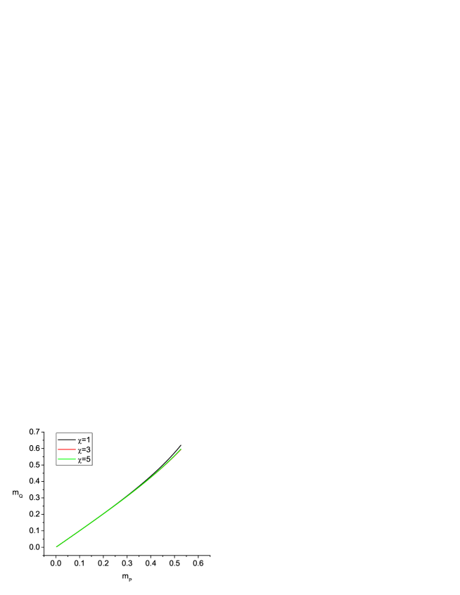
Figure 1: The pole mass of the free domain wall quark, $m_{Q}$, measured in $1/a_{s}$ unit as a function of the propagator bare mass parameter $m_{P}=(1-b(0)^{2})(m+m_{r})$ for three values of the anisotropy parameter $\chi$. Three curves corresponds to $\chi=1$, $3$ and $5$, respectively. We have set $\kappa_{s}=1$, $M_{5}=0.5$ and $L_{s}=8$ in this plot.

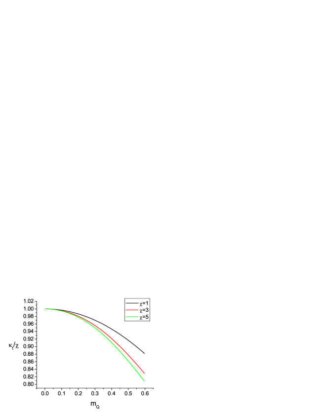
Figure 2: With the same set of parameters as Fig. 1, the value of $\kappa_{t}/\chi$ is shown as a function of the pole mass $m_{Q}$ for $\chi=1$, $3$ and $5$. It is seen that in the massless limit, the expected relation: $\chi=\kappa_{t}/\kappa_{s}$ is recovered for all $\chi$.

To obtain the dispersion relation for the free domain wall fermion, one searches for the pole of the free domain wall fermion propagator. The position of the pole in terms of four-momentum $p_{\mu}$ is given by: $p_{\mu}=(iE_{\mathbf{p}},{\mathbf{p}})$. This then gives the dispersion relation of the fermion: $E_{\mathbf{p}}$ as a function of the three-momentum ${\mathbf{p}}$. The pole mass of the fermion is identified as: $m_{Q}\equiv E_{{\mathbf{p}}=0}=E_{0}$.

In Fig. 1, we have illustrated the pole mass of the massive quark $m_{Q}$ (measured in $1/a_{s}$ unit) as a function of the bare propagator mass parameter $m_{P}$ defined as:

$$m_{P}\equiv(1-b(0)^{2})(m+m_{r})\;,$$ (16)

for three values of anisotropy $\chi$, namely $\chi=1$, $3$ and $5$, respectively. Note that the residue mass is given by $m_{r}=e^{-\alpha_{G}(im_{Q},0,0,0)L_{s}}$, as explained in the appendix. The other relevant parameters in this plot are chosen as: $\kappa_{s}=1$, $M_{5}=0.5$ and $L_{s}=8$. It is seen that the pole mass $m_{Q}$ basically depends on $m_{P}$ linearly for $m_{P}$ values not too large. The nonlinearity only sets in for large bare quark mass values. Also, the dependence of $m_{Q}$ on $m_{P}$ saturates quickly for anisotropy larger than unity. For example, the difference between the case $\chi=3$ and $\chi=5$ is barely visible.

The dispersion relation for the free domain wall fermion is quite complicated. However, for small three lattice momenta: $a_{s}|{\mathbf{p}}|\ll 1$, one finds that:

$$E_{\mathbf{p}}=m_{Q}+{{\mathbf{p}}^{2}\over 2M_{\rm kin}}+O({\mathbf{p}}^{4})\;,$$ (17)

where $M_{\rm kin}$ is the so-called kinetic mass of the quark. To recover normal relativistic dispersion relation for small three lattice momenta, one requires: $m_{Q}=M_{\rm kin}$ which yields a relation among the pole mass and the other parameters in the theory (see Appendix A for the explicit formulae). For the same set of bare parameters as in Fig. 1, we have shown the values of $\kappa_{t}/\chi$ as a function of the pole mass $m_{Q}$ (measured in $1/a_{s}$ unit) in Fig. 2. Note that in a quenched calculation, the anisotropy parameter $\chi$ is in fact fixed by the pure gauge sector. Therefore, once the pole mass of the quark (or equivalently the propagator mass $m_{P}$) and other bare parameters are fixed, one has to tune $\kappa_{t}$ in such a way that the dispersion relation of the fermion resembles the continuum form in the small $a_{s}|{\mathbf{p}}|$ region. Basically one utilizes the relation shown in Fig 2 to find out the appropriate value of $\kappa_{t}$ for a give value of $m_{Q}$. Of course, for vanishing $m_{Q}$, one recovers the expected relation: $\chi=\kappa_{t}/\kappa_{s}$.

4 Fermion Propagator to One-loop

In this section, we outline the basic strategies to calculate the domain wall fermion propagator to one-loop. Numerical results will be provided in the next section. To simplify the presentation here, some explicit formulae for the loop integrals are provided in Appendix B.

4.1 Feynman rules

First of all, one needs the free propagator of the lattice gauge fields [28]. This is obtained by expressing the pure-gauge action (1) (with the tadpole improvement factor $u_{s}$ set to unity) into the gauge potential $A_{\mu}(x)$. One also needs to fix to a particular gauge. We adopt the following gauge-fixing action:

$$S_{gf}=\frac{1}{2\alpha_{g}}\,\frac{1}{\chi}\,\sum_{x}\left[\chi^{2}\partial_{t}(a_{t}A_{t})+\sum_{j}\partial_{j}(a_{s}A_{j})\right]^{2},$$ (18)

where $\alpha_{g}$ is the gauge-fixing parameter. The gauge field measure action and the Fadeev-Popov ghost action do not enter our one-loop calculation.

After performing Fourier transformation of the gauge fields, the quadratic part of the gauge action then has the standard form in momentum space:

$$S^{(0)}_{g}[A_{\mu}]=\frac{1}{2}\,\sum_{\mu\nu}\int_{-\pi}^{\pi}\frac{d^{4}l}{(2\pi)^{4}}\left(\bar{A}_{\mu}(l)\,M_{\mu\nu}(l)\,\bar{A}_{\nu}(-l)\right),$$ (19)

where

$$M_{00} = \chi\,\left[\frac{\chi^{2}}{\alpha_{g}}\hat{l}_{0}^{2}\;+\;\sum_{j}\hat{l}_{j}^{2}\,q_{0j}\right]$$ (20)

$$M_{jj} = \frac{1}{\chi}\,\left[\frac{1}{\alpha_{g}}\hat{l}_{j}^{2}\;+\;\chi^{2}\,\hat{l}_{0}^{2}\,q_{0j}\;+\;\sum_{j^{\prime}\neq j}\hat{l}_{j^{\prime}}^{2}\,q_{j^{\prime}j}\right]$$ (21)

$$M_{i\neq j} = \frac{1}{\chi}\,\left[\frac{1}{\alpha_{g}}\hat{l}_{i}\hat{j}_{j}\;-\;\hat{l}_{i}\hat{l}_{j}\,q_{ij}\right]$$ (22)

$$M_{0j} = M_{j0}=\chi\,\left[\frac{1}{\alpha_{g}}\hat{l}_{0}\hat{l}_{j}\;-\;\hat{l}_{0}\hat{l}_{j}\,q_{0j}\right]$$ (23)

with lattice momentum defined as: $\hat{l}_{\mu}\equiv 2\,\sin(\frac{l_{\mu}}{2})$. The quantities $q_{\mu\nu}$ appearing in the above equations are given by:

$$q_{ij}=1\;+\;\frac{1}{12}\,(\hat{l}^{2}_{i}+\hat{l}^{2}_{j})\qquad i\neq j\;,\;\;q_{0j}=1\;+\;\frac{1}{12}\,\hat{l}^{2}_{j}\;.$$ (24)

Using these notations, the free gauge field propagator is expressed as:

$$D_{\mu\nu}(l)=M^{-1}_{\mu\nu}=\frac{1}{(\hat{l}^{2})^{2}}\left[\alpha_{g}\hat{l}_{\mu}\hat{l}_{\nu}\chi+\frac{f^{\mu\nu}(\hat{l}_{\rho},q_{\rho\sigma},\chi)}{f_{D}(\hat{l}_{\rho},q_{\rho\sigma},\chi)}\right],$$ (25)

For simplicity, we set $\alpha_{g}=1$ in the following calculation. The explicit expressions for $f^{\mu\nu}$ and $f_{D}$ maybe found in the literature [28].

The vertex functions can be obtained from the corresponding expression in the isotropic lattice case, which was given in Ref. [22]. After making necessary modifications to the case of anisotropic lattice, we have for the one gluon emission vertex:

$$V_{1}(k,p,l;a,\mu)=-igT^{a}\kappa_{\mu}\left[\gamma_{\mu}\cos{1\over 2}(p_{\mu}-k_{\mu})+i\sin{1\over 2}(p_{\mu}-k_{\mu})\right]\;,$$ (26)

where $k$, $p$ and $l=-(k+p)$ are the momenta for the anti-quark, quark and the gluon field, respectively; $a$ and $\mu$ representing the color and Lorentz index of the gluon. The anti-quark, quark and two-gluon vertex is given by:

$$V_{2}(k,p,l_{1},l_{2};a,b,\mu,\nu) = {g^{2}\over 2}{\kappa_{\mu}\over 2}\{T^{a},T^{b}\}\left[i\gamma_{\mu}\sin{1\over 2}(p_{\mu}-k_{\mu})\right.$$ (27)

$$+ \left.\cos{1\over 2}(p_{\mu}-k_{\mu})\right]\delta_{\mu\nu}\;,$$

where $k$, $p$, $l_{1}$ and $l_{2}$ are the momenta for anti-quark, quark and the two gluon fields with the energy-momentum conservation constraint: $k+p+l_{1}+l_{2}=0$. $\mu$, $\nu$, $a$ and $b$ are the Lorentz and color indices for the two gluons. Expressions for other vertices will not be needed in our one-loop calculation.

4.2 Fermion self-energy

To one-loop order, two Feynman diagrams contribute to fermion self-energy: the tadpole diagram and the half-circle diagram. Thus, the 1PI fermion 2-point vertex function reads:

$$V^{(2)}_{\rm 1-loop}(p)_{s,s^{\prime}}=\left[i\sum_{\mu}\kappa_{\mu}\gamma_{\mu}\sin p_{\mu}+W^{+}(p)P_{R}+W^{-}(p)P_{L}-\Sigma(p)\right]_{s,s^{\prime}}$$ (28)

where the fermion self-energy $\Sigma(p)$ receives contributions from the tadpole and the half-circle diagrams, respectively:

$$\Sigma(p)=\Sigma^{\rm tadpole}(p)+\Sigma^{\rm half-circle}(p).$$ (29)

Using the Feynman rules given in the previous section, the contribution from the tadpole diagram can be written as:

$$\Sigma^{\rm tadpole}(p) = \frac{1}{2}g^{2}C_{F}\sum_{\mu}\kappa_{\mu}(i\gamma_{\mu}\sin p_{\mu}+\cos p_{\mu})$$ (30)

$$\times \int_{-\pi}^{\pi}\frac{d^{4}l}{(2\pi)^{4}}\frac{1}{(\chi^{2}\hat{l}^{2}_{0}+\sum_{j}\hat{l}^{2}_{j})^{2}}(\hat{l}^{2}_{\mu}\chi+\frac{f^{\mu\mu}}{f_{D}})\delta_{s,s^{\prime}}\;,$$

$$= -\left[\sum_{\mu}i\gamma_{\mu}\tilde{p}_{\mu}I_{\rm tad,\mu}(s,s^{\prime})+M_{\rm tad}(s,s^{\prime})\right]$$

where the explicit expressions for $I_{\rm tad,\mu}(s,s^{\prime})$ and $M_{\rm tad}(s,s^{\prime})$ are given by Eq. (B) in appendix B. Note that both $I_{\rm tad,\mu}(s,s^{\prime})$ and $M_{\rm tad}(s,s^{\prime})$ are independent of the quark mass explicitly. They are diagonal in the fifth dimensional index and can be computed by numerical integration.

For the half circle diagram, the contribution can be written as:

$$\Sigma^{\rm half-circle}_{s,s^{\prime}}(p) = \int_{-\pi}^{\pi}\frac{d^{4}l}{(2\pi)^{4}}\sum_{\mu}(-g^{2}C_{F})\kappa^{2}_{\mu}\left\{\gamma_{\mu}\cos(\frac{l+p}{2})_{\mu}+i\sin(\frac{l+p}{2})_{\mu}\right\}$$ (31)

$$\times S_{F}(l)_{s,s^{\prime}}\times\left\{\gamma_{\mu}\cos(\frac{l+p}{2})_{\mu}+i\sin(\frac{l+p}{2})_{\mu}\right\}$$

$$\times \left\{\frac{1}{(\chi^{2}(\widehat{p_{0}-l_{0}})^{2}+\sum_{j}(\widehat{p_{j}-l_{j}})^{2})^{2}}\left[\chi(\widehat{p_{\mu}-l_{\mu}})^{2}+\frac{f^{\mu\mu}}{f_{D}}\right]\right\}\;.$$

Note that although $\Sigma^{\rm tadpole}(p)$ is proportional to the unit matrix in the fifth dimensional space, $\Sigma^{\rm half-circle}_{s,s^{\prime}}(p)$ is non-trivial due to the fermion propagator $S_{F}(l)_{ss^{\prime}}$ which is given by Eq. (9) in the previous section. To simplify our one-loop calculation, we have neglected the effects caused by the finite extension of the fifth dimension in the following calculation, i.e. we have set: $m_{r}=e^{-\alpha_{G}L_{s}}\simeq 0$ in the quark propagator $S_{F}(l)_{ss^{\prime}}$. However, in order to study the quark mass effects, we have kept the bare quark mass parameter $m$ non-zero.

The calculation of $\Sigma^{\rm half-circle}_{s,s^{\prime}}(p)$ is somewhat different in the massive and the massless cases. If the fermion is massless, it is well-known that $\Sigma^{\rm half-circle}_{s,s^{\prime}}(p)$ contains infra-red divergences [28, 22]. If the fermion is massive, no infra-red divergence shows up in this contribution. In the massive fermion case, since there is no infra-red divergence, the expression given in Eq. (31) can be evaluated directly by numerical integration methods. In the massless case, however, the infra-red divergent part (which can be computed analytically) has to be subtracted from the self-energy contribution $\Sigma^{\rm half-circle}_{s,s^{\prime}}(p)$ before it can be evaluated numerically. For the physical quantities in the massive fermion case, we denote them as $f(m)$. For the same quantity in the massless case, we denote the subtracted expression as:

$$f_{\rm finite}=f(m=0)-f_{\log}\;,$$ (32)

where $f$ represents some physical quantity and $f_{\log}$ contains the logarithmical infra-red divergent part to be removed from $f(m=0)$. Usually, $f_{\log}$ is taken to be the corresponding infra-red divergent contribution in the continuum which can be computed analytically. After the subtraction of infra-red divergent part, $f_{\rm finite}$ is free of infra-red divergences and can be evaluated numerically.

For the half-circle contribution in the massive case, we obtain:

$$\Sigma^{\rm half-circle}_{s,s^{\prime}}(m) = -i\sum_{\mu}\gamma_{\mu}\tilde{p}_{\mu}\left([I^{+}_{\mu}(m)]_{s,s^{\prime}}P_{R}+[I^{-}_{\mu}(m)]_{s,s^{\prime}}P_{L}\right)$$ (33)

$$-\left([M^{+}(m)]_{s,s^{\prime}}P_{R}+[M^{-}(m)]_{s,s^{\prime}}P_{L}\right)\;.$$

In the massless case, after separating the infra-red divergent part, the half-circle contribution are obtained as:

$$\Sigma^{\rm half-circle}_{s,s^{\prime}} = -i\sum_{\mu}\gamma_{\mu}\tilde{p}_{\mu}\left[\left(I_{\rm finite,\mu}^{+}(s,s^{\prime})+I_{\rm log,\mu}^{+}(s,s^{\prime})\right)P_{R}\right.$$ (34)

$$+\left.\left(I_{\rm finite,\mu}^{-}(s,s^{\prime})+I_{\rm log,\mu}^{-}(s,s^{\prime})\right)P_{L}\right]$$

$$-\left[\left(M_{\rm finite}^{+}(s,s^{\prime})+M_{\rm log}^{+}(s,s^{\prime})\right)P_{R}\right.$$

$$+\left.(\left(M_{\rm finite}^{-}(s,s^{\prime})+M_{\rm log}^{-}(s,s^{\prime})\right)P_{L}\right]$$

where explicit formulae for the quantities appearing in the above formulae can be found in appendix B.

Combining the tadpole and the half-circle contributions, we may express the effective action of the domain wall fermion as:

$$\Gamma^{(2)}=\bar{\psi}(-p)_{s}\left[\sum_{\mu}i\gamma_{\mu}\tilde{p}_{\mu}\left(Z^{+}_{\mu}P_{R}+Z^{-}_{\mu}P_{L}\right)+\overline{W}^{+}P_{R}+\overline{W}^{-}P_{L}\right]_{s,s^{\prime}}\psi(p)_{s}^{\prime}$$ (35)

where the matrices $Z^{\pm}_{\mu}$ and $\bar{W}^{\pm}$ are given by:

$$Z^{\pm}_{\mu}(s,s^{\prime}) = \delta_{s,s^{\prime}}+I_{\rm tad,\mu}(s,s^{\prime})+[I^{\pm}_{\mu}(m)]_{s,s^{\prime}}\;,$$

$$\overline{W}^{\pm}(s,s^{\prime}) = W^{\pm}(0)(s,s^{\prime})+M_{\rm tad}(s,s^{\prime})+[M^{\pm}(m)]_{s,s^{\prime}}\;.$$ (36)

in the massive case. The quantities $[I^{\pm}_{\mu}(m)]_{s,s^{\prime}}$ and $[M^{\pm}(m)]_{s,s^{\prime}}$ are replaced by the sum of a finite part and an infra-red divergent part in the massless case:

$$Z^{\pm}_{\mu}(s,s^{\prime}) = \delta_{s,s^{\prime}}+I_{\rm tad,\mu}(s,s^{\prime})+I^{\pm}_{\log,\mu}(s,s^{\prime})+I^{\pm}_{\rm finite,\mu}(s,s^{\prime})\;,$$

$$\overline{W}^{\pm}(s,s^{\prime}) = W^{\pm}(0)(s,s^{\prime})+M_{\rm tad}(s,s^{\prime})+M^{\pm}_{\rm log}(s,s^{\prime})+M^{\pm}_{\rm finite}(s,s^{\prime})\;.$$ (37)

The explicit formulae for the tadpole contributions $I_{\rm tad,\mu}(s,s^{\prime})$, $M_{\rm tad}(s,s^{\prime})$ and the half-circle contributions $[I^{\pm}_{\mu}(m)]_{s,s^{\prime}}$, $[M^{\pm}(m)]_{s,s^{\prime}}$ $M^{\pm}_{\rm log}(s,s^{\prime})$, $M^{\pm}_{\rm finite}(s,s^{\prime})$, $I^{\pm}_{\log,\mu}(s,s^{\prime})$, $I^{\pm}_{\rm finite,\mu}(s,s^{\prime})$ can be found in appendix B.

4.3 Wave-function and mass renormalization of the chiral mode

We are concerned with the renormalization of the chiral modes which are bound to the walls. To obtain this information, it is better to use a new basis, $\psi^{d}(p)$, which diagonalizes the mass matrices $\overline{W}^{\pm}$ in Eq. (4.2). This new basis is related to the old one via:

$$\psi^{d}_{s}(p)={\mathcal{U}}_{s,s^{\prime}}P_{R}\psi_{s^{\prime}}(p)+{\mathcal{V}}_{s,s^{\prime}}P_{L}\psi_{s^{\prime}}(p),$$ (38)

where the two unitary matrices ${\mathcal{U}}$ and ${\mathcal{V}}$ satisfy

$$\left[{\mathcal{U}}\overline{W}^{-}\overline{W}^{+}{\mathcal{U}}^{\dagger}\right]_{s,s^{\prime}}=M_{s}^{2}\delta_{s,s^{\prime}}\;,\;\;\left[{\mathcal{V}}\overline{W}^{+}\overline{W}^{-}{\mathcal{V}}^{\dagger}\right]_{s,s^{\prime}}=M_{s}^{2}\delta_{s,s^{\prime}}\;.$$ (39)

Under this new basis, the effective action of the fermion becomes:

$$\Gamma^{(2)} = \bar{\psi}^{d}(-p)_{s}\Bigg{[}\sum_{\mu}i\gamma_{\mu}\tilde{p}_{\mu}\left({\mathcal{U}}Z^{+}_{\mu}{\mathcal{U}}^{\dagger}P_{R}+{\mathcal{V}}Z^{-}_{\mu}{\mathcal{V}}^{\dagger}P_{L}\right)$$ (40)

$$+ {\mathcal{V}}\overline{W}^{+}{\mathcal{U}}^{\dagger}P_{R}+{\mathcal{U}}\overline{W}^{-}{\mathcal{V}}^{\dagger}P_{L}\Bigg{]}_{s,s^{\prime}}\psi^{d}(p)_{s^{\prime}}\;.$$

The unitary matrices ${\mathcal{U}}$, ${\mathcal{V}}$ and the corresponding eigenvalues $(M^{2})_{s}$ can be calculated to 1-loop level:

$${\mathcal{U}} = (1+g^{2}{\mathcal{U}}^{(1)}){\mathcal{U}}^{(0)}\;,\;\;{\mathcal{V}}=(1+g^{2}{\mathcal{V}}^{(1)}){\mathcal{V}}^{(0)}\;,$$ (41)

$$(M^{2})_{s} = (M^{2}_{0})_{s}+g^{2}(M^{2}_{1})_{s}\;.$$ (42)

where tree-level matrices ${\mathcal{U}}_{0}$ and ${\mathcal{V}}_{0}$ are defined in Eq. (14).

After diagonalization of the mass matrix, the effective action for the chiral mode field $\psi^{d}(p)_{L_{s}-1}=\chi_{0}(p)$ becomes:

$$\bar{\chi}_{0}(-p)\left[\sum_{\mu}i\gamma_{\mu}\tilde{p}_{\mu}\left(\tilde{Z}_{+,\mu}P_{R}+\tilde{Z}_{-,\mu}P_{L}\right)+\tilde{W}_{+}P_{R}+\tilde{W}_{-}P_{L}\right]\chi_{0}(p)\;,$$ (43)

where

$$\tilde{Z}_{\pm,\mu} = 1+g^{2}\left(I^{d}_{\pm,\rm tad,\mu}+I^{d}_{\pm,\mu}(m)\right)_{L_{s}-1,L_{s}-1}\;,$$ (44)

$$\tilde{W}_{\pm} = -m_{P}\left[1+g^{2}\left(M^{d}_{\pm,\rm tad}+M^{d}_{\pm}(m)\right)_{L_{s}-1,L_{s}-1}\right]\;.$$ (45)

The above formulae work for the massive case. In the massless case, one has to modify the right-hand side of Eq. (44) and Eq. (45) accordingly as specified by Eq. (32). Note that chiral symmetry ensures that the effective quark mass term is renormalized by a multiplicative factor, i.e. there is no additive renormalization. The matrix elements of various $I^{d}_{\mu}$ and $M^{d}$ in the above expressions are given explicitly by:

$$g^{2}I^{d}_{+,\rm tad,\mu} = {\mathcal{U}}^{(0)}I_{\rm tad,\mu}{\mathcal{U}}^{(0)\dagger}\;,\;\;g^{2}I^{d}_{-,\rm tad,\mu}={\mathcal{V}}^{(0)}I_{\rm tad,\mu}{\mathcal{V}}^{(0)\dagger}\;,$$

$$g^{2}I^{d}_{+,\mu} = {\mathcal{U}}^{(0)}I_{\mu}^{+}{\mathcal{U}}^{(0)\dagger}\;,\;\;g^{2}I^{d}_{-,\mu}={\mathcal{V}}^{(0)}I_{\mu}^{-}{\mathcal{V}}^{(0)\dagger}\;,$$

$$g^{2}I^{d}_{+,\rm log,\mu} = {\mathcal{U}}^{(0)}I_{\rm log,\mu}^{+}{\mathcal{U}}^{(0)\dagger}\;,\;\;g^{2}I^{d}_{-,\rm log,\mu}={\mathcal{V}}^{(0)}I_{\rm log,\mu}^{-}{\mathcal{V}}^{(0)\dagger}\;,$$

$$g^{2}I^{d}_{+,\rm finite,\mu} = {\mathcal{U}}^{(0)}I_{\rm finite,\mu}^{+}{\mathcal{U}}^{(0)\dagger}\;,\;\;g^{2}I^{d}_{-,\rm finite,\mu}={\mathcal{V}}^{(0)}I_{\rm finite,\mu}^{-}{\mathcal{V}}^{(0)\dagger}\;.$$ (46)

$$g^{2}m_{P}M^{d}_{+,\rm tad} = {\mathcal{V}}^{(0)}M_{\rm tad}{\mathcal{U}}^{(0)\dagger}\;,\;\;g^{2}m_{P}M^{d}_{-,\rm tad}={\mathcal{U}}^{(0)}M_{\rm tad}{\mathcal{V}}^{(0)\dagger}\;,$$

$$g^{2}m_{P}M^{d}_{+} = {\mathcal{V}}^{(0)}M^{+}{\mathcal{U}}^{(0)\dagger}\;,\;\;g^{2}m_{P}M^{d}_{-}={\mathcal{U}}^{(0)}M^{-}{\mathcal{V}}^{(0)\dagger}\;,$$

$$g^{2}m_{P}M^{d}_{+,\rm log} = {\mathcal{V}}^{(0)}M_{\rm log}^{+}{\mathcal{U}}^{(0)\dagger}\;,\;\;g^{2}m_{P}M^{d}_{-,\rm log}={\mathcal{U}}^{(0)}M_{\rm log}^{-}{\mathcal{V}}^{(0)\dagger}\;,$$

$$g^{2}m_{P}M^{d}_{+,\rm finite} = {\mathcal{V}}^{(0)}M_{\rm finite}^{+}{\mathcal{U}}^{(0)\dagger}\;,\;\;g^{2}m_{P}M^{d}_{-,\rm finite}={\mathcal{U}}^{(0)}M_{\rm finite}^{-}{\mathcal{V}}^{(0)\dagger}\;.$$ (47)

It is also easy to show that:

$$(I^{d}_{+,\rm tad,\mu})_{L_{s}-1,L_{s}-1} = (I^{d}_{-,\rm tad,\mu})_{L_{s}-1,L_{s}-1}\equiv I^{d}_{\rm tad,\mu}\;,$$

$$(I^{d}_{+,\mu})_{L_{s}-1,L_{s}-1} = (I^{d}_{-,\mu})_{L_{s}-1,L_{s}-1}\equiv I^{d}_{\mu}\;,$$

$$(I^{d}_{+,\rm log,\mu})_{L_{s}-1,L_{s}-1} = (I^{d}_{-,\rm log,\mu})_{L_{s}-1,L_{s}-1}\equiv I^{d}_{\rm log,\mu}\;,$$

$$(I^{d}_{+,\rm finite,\mu})_{L_{s}-1,L_{s}-1} = (I^{d}_{-,\rm finite,\mu})_{L_{s}-1,L_{s}-1}\equiv I^{d}_{\rm finite,\mu}\;,$$

$$(M^{d}_{+,\rm tad})_{L_{s}-1,L_{s}-1} = (M^{d}_{-,\rm tad})_{L_{s}-1,L_{s}-1}\equiv M^{d}_{\rm tad}\;,$$

$$(M^{d}_{+})_{L_{s}-1,L_{s}-1} = (M^{d}_{-})_{L_{s}-1,L_{s}-1}\equiv M^{d}\;,$$

$$(M^{d}_{+,\rm log})_{L_{s}-1,L_{s}-1} = (M^{d}_{-,\rm log})_{L_{s}-1,L_{s}-1}\equiv M^{d}_{\rm log}\;,$$

$$(M^{d}_{+,\rm finite})_{L_{s}-1,L_{s}-1} = (M^{d}_{-,\rm finite})_{L_{s}-1,L_{s}-1}\equiv M^{d}_{\rm finite}\;,$$ (48)

Thus one obtains: $\tilde{Z}_{+,\mu}=\tilde{Z}_{-,\mu}\equiv\tilde{Z}_{\mu}$ and $\tilde{W}_{+}=\tilde{W}_{-}\equiv\tilde{W}$. Using the above notations, we get for the wave-function and mass renormalization factors:

$$\tilde{Z}_{\mu} = 1+g^{2}\left(I^{d}_{\rm tad,\mu}+I^{d}_{\mu}(m)\right)\;,$$ (49)

$$\tilde{W}_{\pm} = -m_{P}\left[1+g^{2}\left(M^{d}_{\rm tad}+M^{d}(m)\right)\right]\;,$$ (50)

in the massive case and

$$\tilde{Z}_{\mu} = 1+g^{2}\left(I^{d}_{\rm tad,\mu}+I^{d}_{\log,\mu}+I^{d}_{\rm finite,\mu}\right)\;,$$ (51)

$$\tilde{W}_{\pm} = -m_{P}\left[1+g^{2}\left(M^{d}_{\rm tad}+M^{d}_{\log}+M^{d}_{\rm finite}\right)\right]\;,$$ (52)

in the massless case.

The tadpole contributions $I^{d}_{\rm tad,\mu}$ and $M^{d}_{\rm tad}$ can be obtained numerically by using the definition (4.3) and the explicit expressions of $I_{\rm tad,\mu}(s,s^{\prime})$ and $M_{\rm tad}(s,s^{\prime})$ given in appendix B (c.f. Eq. (B)). Using the definition of ${\mathcal{U}}^{(0)}$ and ${\mathcal{V}}^{(0)}$, we get:

$$I^{d}_{\rm tad,\mu}=-C_{F}\frac{1}{2}\int_{-\pi}^{\pi}\frac{d^{4}l}{(2\pi)^{4}}\frac{1}{(\chi^{2}\hat{l}^{2}_{0}+\sum_{j}\hat{l}^{2}_{j})^{2}}(\hat{l}^{2}_{\mu}\chi+\frac{f^{\mu\mu}}{f_{D}})\;.$$ (53)

and if we define $M^{0}_{\rm tad}$ as

$$M^{0}_{\rm tad}=-C_{F}\frac{1}{2}\int_{-\pi}^{\pi}\frac{d^{4}l}{(2\pi)^{4}}\sum_{\mu}\frac{\kappa_{\mu}}{(\chi^{2}\hat{l}^{2}_{0}+\sum_{j}\hat{l}^{2}_{j})^{2}}(\hat{l}^{2}_{\mu}\chi+\frac{f^{\mu\mu}}{f_{D}})\;,$$ (54)

we arrive at:

$$M^{d}_{\rm tad}=2e^{-\alpha}/((1-b^{2}(0))(1+m^{2}e^{-2\alpha}))M^{0}_{\rm tad}\;,$$ (55)

where the parameter $\alpha$ is exponential decaying rate for the chiral mode in the fifth dimension. Using these equations, numerical values of $I^{d}_{\rm tad,\mu}$ and $M^{d}_{\rm tad}$ will be presented in the next section.

We now proceed to evaluate the half-circle contributions: $I^{d}_{\mu}$ and $M^{d}$. If we use the shorthand notation:

$$\langle F\rangle_{\mathcal{U}}\equiv\sum_{s,s^{\prime}}({\mathcal{U}}^{(0)})_{L_{s}-1,s}F(s,s^{\prime})({\mathcal{U}}^{(0)})_{L_{s}-1,s^{\prime}}$$

and a similarly notation associated with ${\mathcal{V}}^{(0)}$, we have:

$$\langle G_{L}\rangle_{\mathcal{U}} = B\left[\frac{\sinh\alpha_{G}-\sinh\alpha}{\cosh\alpha_{G}-\cosh\alpha}-(1-e^{-2\alpha})\frac{{\mathcal{N}}_{1}}{{\mathcal{D}}}\right]=\langle G_{R}\rangle_{\mathcal{V}}\equiv\widetilde{G_{L}}\;,$$

$$\langle G_{R}\rangle_{\mathcal{U}} = B\left[\frac{\sinh\alpha_{G}-\sinh\alpha}{\cosh\alpha_{G}-\cosh\alpha}-(1-e^{-2\alpha})\frac{{\mathcal{N}}_{2}}{{\mathcal{D}}}\right]=\langle G_{L}\rangle_{\mathcal{V}}\equiv\widetilde{G_{R}}\;,$$

$$\langle W_{0}^{+}G_{L}\rangle_{\mathcal{U}} = \langle W_{0}^{-}G_{R}\rangle_{\mathcal{V}}=(e^{-\alpha}-b)\widetilde{G_{R}}+R_{0}+R_{1}\;,$$

$$\langle W_{0}^{+}G_{L}\rangle_{\mathcal{V}} = \langle W_{0}^{-}G_{R}\rangle_{\mathcal{U}}=(e^{-\alpha}-b)\widetilde{G_{R}}+R_{0}+R_{2}\;,$$

where:

$${\mathcal{N}}_{1} = (1-m^{2})(e^{\alpha_{G}}-b)+(1-m^{2})(e^{-\alpha_{G}}-b)m^{2}e^{-2\alpha}+4bm^{2}\sinh\alpha_{G}e^{-\alpha}$$

$${\mathcal{N}}_{2} = (1-m^{2})(e^{-\alpha_{G}}-b)+(1-m^{2})(e^{\alpha_{G}}-b)m^{2}e^{-2\alpha}+4bm^{2}\sinh\alpha_{G}e^{-\alpha}$$

$${\mathcal{D}} = (1+m^{2}e^{-2\alpha})\left[(e^{-\alpha_{G}}-b)+m^{2}(be^{-2\alpha_{G}}-e^{-\alpha_{G}})\right](e^{\alpha_{G}}-e^{-\alpha})^{2}$$

$$R_{0} = \frac{1-e^{-2\alpha}}{1+m^{2}e^{-2\alpha}}\frac{1}{(1-e^{-(\alpha+\alpha_{G})})^{2}}\left\{Bm^{2}(1-e^{-2\alpha_{G}})e^{-3\alpha}\right.$$

$$- \left.A_{m}me^{\alpha_{G}}(e^{-\alpha_{G}}+2e^{-\alpha}-2e^{-\alpha_{G}}e^{-2\alpha}-e^{-3\alpha})\right\}$$

$$R_{1} = -A_{m}m\frac{1-e^{-2\alpha}}{1+m^{2}e^{-2\alpha}}\frac{m^{2}e^{-2\alpha}}{1-e^{-(\alpha+\alpha_{G})}}$$

$$R_{2} = -A_{m}m\frac{1-e^{-2\alpha}}{1+m^{2}e^{-2\alpha}}\frac{1}{1-e^{-(\alpha+\alpha_{G})}}$$

Using the above notations, after some algebra, $I^{d}_{\mu}$ is found to be:

$$I^{d}_{\mu}(m) = C_{F}\int\frac{d^{4}l}{(2\pi)^{4}}\Biggl{\{}\Biggl{[}\kappa_{\mu}\left(\cos l_{\mu}((e^{-\alpha}-b)\widetilde{G_{R}}+R_{0}+\frac{R_{1}+R_{2}}{2})\right.$$ (56)

$$+ \left.\frac{1}{2}\kappa_{\mu}\sin^{2}l_{\mu}(\widetilde{G_{L}}+\widetilde{G_{R}})\right)\Biggr{]}\frac{\chi\hat{l}^{2}_{\mu}+\frac{f^{\mu\mu}(l)}{f_{D}(l)}}{(\chi^{2}\hat{l}^{2}_{0}+\sum_{j}\hat{l}^{2}_{j})^{2}}$$

$$+ \Biggl{[}\left(\kappa_{\mu}((e^{-\alpha}-b)\widetilde{G_{R}}+R_{0}+\frac{R_{1}+R_{2}}{2})-2\kappa^{2}_{\mu}\cos^{2}l_{\mu}/2\widetilde{G_{L}}\right)$$

$$\times \left(\frac{4(\chi^{2})^{\delta_{\mu 0}}}{\chi^{2}\hat{l}^{2}_{0}+\sum_{j}\hat{l}^{2}_{j}}(\chi\hat{l}^{2}_{\mu}+\frac{f^{\mu\mu}(l)}{f_{D}(l)})-2\chi-\frac{f^{\mu}_{\mu}(l)}{f_{D}(l)}+\frac{f^{D}_{\mu}(l)f^{\mu\mu}(l)}{f^{2}_{D}(l)}\right)$$

$$- 2\chi\kappa^{2}_{\mu}\left(\sin^{2}l_{\mu}/2\widetilde{G_{R}}+\cos^{2}l_{\mu}/2\widetilde{G_{L}}\right)$$

$$+ \sum_{\nu}\kappa^{2}_{\nu}\left(\sin^{2}l_{\nu}/2\widetilde{G_{R}}+\cos^{2}l_{\nu}/2\widetilde{G_{L}}\right)$$

$$\times \left(\frac{4(\chi^{2})^{\delta_{\mu 0}}}{\chi^{2}\hat{l}^{2}_{0}+\sum_{j}\hat{l}^{2}_{j}}(\chi\hat{l}^{2}_{\nu}+\frac{f^{\nu\nu}(l)}{f_{D}(l)})-\frac{f^{\nu}_{\mu}(l)}{f_{D}(l)}+\frac{f^{D}_{\mu}(l)f^{\nu\nu}(l)}{f^{2}_{D}(l)}\right)\Biggr{]}$$

$$\times \frac{\sin^{2}l_{\mu}}{(\chi^{2}\hat{l}^{2}_{0}+\sum_{j}\hat{l}^{2}_{j})^{2}}\Biggr{\}}$$

In the massless case, what needs to be calculated numerically is the subtracted finite part $I^{d}_{\rm finite,\mu}$ defined as:

$$I^{d}_{\rm finite,\mu} = I^{d}_{\mu}(m=0)-C_{F}\frac{(1-b^{2}(0))(1-e^{-2\alpha})}{(1-b(0)e^{-\alpha})^{2}}$$ (57)

$$\times \int\frac{d^{4}l}{(2\pi)^{4}}\frac{4\chi(\chi^{2})^{\delta_{\mu 0}}l^{2}_{\mu}\theta(\pi^{2}-(\chi^{2}l^{2}_{0}+\sum_{j}l^{2}_{j}))}{(\chi^{2}l^{2}_{0}+\sum_{j}l^{2}_{j})^{3}}\;.$$

The infra-red divergent part that is subtracted from $I^{d}_{\mu}(0)$ is denoted as $I^{d}_{\log,\mu}$ and can be obtained analytically by using Eq. (86) and the definition (4.3).

For the contribution $M^{d}$, we have:

$$({\mathcal{V}}^{(0)}0G_{L}{\mathcal{U}}^{(0)\dagger})_{L_{s}-1,L_{s}-1} = ({\mathcal{U}}^{(0)}G_{R}{\mathcal{V}}^{(0)\dagger})_{L_{s}-1,L_{s}-1}=\widetilde{G^{M}_{L}}\;,$$

$$({\mathcal{V}}^{(0)}G_{R}{\mathcal{U}}^{(0)\dagger})_{L_{s}-1,L_{s}-1} = ({\mathcal{U}}^{(0)}G_{R}{\mathcal{V}}^{(0)\dagger})_{L_{s}-1,L_{s}-1}=\widetilde{G^{M}_{R}}\;.$$ (58)

One also verifies that:

$$\widetilde{G^{M}_{L}} = \widetilde{G^{M}_{R}}\equiv-m_{P}\widetilde{G^{M}}$$ (59)

$$= -m_{P}\frac{(1-e^{-2\alpha})B}{(1-b^{2}(0))(1+m^{2}e^{-2\alpha})}\left[2\frac{1+e^{-(\alpha_{G}+\alpha)}}{1-e^{-(\alpha_{G}+\alpha)}}\frac{e^{-\alpha}}{1-e^{-2\alpha}}\right.$$

$$+ \left.\frac{\Delta^{-1}}{(1-e^{-(\alpha_{G}+\alpha)})^{2}}\left(2e^{-\alpha}(1-m^{2})(\cosh\alpha_{G}-b)+\frac{1+m^{2}e^{-2\alpha}}{B}\right)\right]\;.$$

We also find:

$$({\mathcal{V}}^{(0)}W^{+}G_{L}{\mathcal{U}}^{(0)\dagger})_{L_{s}-1,L_{s}-1} = ({\mathcal{U}}^{(0)}W^{-}G_{R}{\mathcal{V}}^{(0)\dagger})_{L_{s}-1,L_{s}-1}$$

$$= -m_{P}\left((e^{-\alpha}-b)\widetilde{G^{M}}+R_{0}^{M}+R_{1}^{M}\right)\;,$$

$$({\mathcal{V}}^{(0)}W^{-}G_{R}{\mathcal{U}}^{(0)\dagger})_{L_{s}-1,L_{s}-1} = ({\mathcal{U}}^{(0)}W^{+}G_{L}{\mathcal{V}}^{(0)\dagger})_{L_{s}-1,L_{s}-1}$$

$$= -m_{P}\left((e^{-\alpha}-b)\widetilde{G^{M}}+R_{0}^{M}+R_{2}^{M}\right)\;,$$

$$({\mathcal{V}}^{(0)}W^{+}(0){\mathcal{U}}^{(0)\dagger})_{L_{s}-1,L_{s}-1} = ({\mathcal{U}}^{(0)}W^{-}(0){\mathcal{V}}^{(0)\dagger})_{L_{s}-1,L_{s}-1}$$

$$= -m_{P}\frac{1-e^{-2\alpha}}{(1-b^{2}(0))(1+m^{2}e^{-2\alpha})}$$

$$\times \left(1+\frac{2e^{-\alpha}(e^{-\alpha}-b(0))}{1-e^{-2\alpha}}\right)\;,$$

where

$$R_{0}^{M} = \frac{(1-e^{-2\alpha})B\Delta^{-1}}{(1-b^{2}(0))(1+m^{2}e^{-2\alpha})}\frac{e^{-\alpha}}{(1-e^{-(\alpha_{G}+\alpha)})^{2}}$$

$$\times (1-m^{2})\left[(e^{-\alpha_{G}}-e^{-\alpha})(e^{\alpha_{G}}-b)+(e^{\alpha_{G}}-e^{-\alpha})(e^{-\alpha_{G}}-b)\right]$$

$$R_{1}^{M} = \frac{1-e^{-2\alpha}}{(1-b^{2}(0))(1+m^{2}e^{-2\alpha})}$$

$$\times \left\{B\frac{1+2e^{-(\alpha_{G}+\alpha)}}{1-e^{-(\alpha_{G}+\alpha)}}+{1\over\Delta}\left(B\frac{(1-m^{2})(e^{\alpha_{G}}-b)}{1-e^{-(\alpha_{G}+\alpha)}}\right.\right.$$

$$+ \left.\left.\frac{(e^{-\alpha_{G}}-e^{-\alpha})m^{2}e^{-2\alpha}+e^{\alpha_{G}}-e^{-\alpha}}{(1-e^{-(\alpha_{G}+\alpha)})^{2}}+\frac{m^{2}e^{-\alpha}}{1-e^{-(\alpha_{G}+\alpha)}}\right)\right\}\;,$$

$$R_{2}^{M} = \frac{1-e^{-2\alpha}}{(1-b^{2}(0))(1+m^{2}e^{-2\alpha})}$$

$$\times \left\{B\frac{m^{2}e^{-2\alpha}+2e^{-(\alpha_{G}+\alpha)}}{1-e^{-(\alpha_{G}+\alpha)}}+{1\over\Delta}\left(B\frac{(1-m^{2})(e^{\alpha_{G}}-b)}{1-e^{-(\alpha_{G}+\alpha)}}m^{2}e^{-2\alpha}\right.\right.$$

$$+ \left.\left.\frac{(e^{\alpha_{G}}-e^{-\alpha})m^{2}e^{-2\alpha}+e^{-\alpha_{G}}-e^{-\alpha}}{(1-e^{-(\alpha_{G}+\alpha)})^{2}}+\frac{m^{2}e^{-\alpha}}{1-e^{-(\alpha_{G}+\alpha)}}\right)\right\}\;.$$

Using the above expressions, the quantity $M^{d}$ is found to be:

$$M^{d} = g^{2}C_{F}\int\frac{d^{4}l}{(2\pi)^{4}}\sum_{\mu}\kappa^{2}_{\mu}\Biggl{[}\cos^{2}l_{\mu}/2\left((e^{-\alpha}-b)\widetilde{G^{M}}+R_{0}^{M}+R_{1}^{M}\right)$$ (60)

$$- \sin^{2}l_{\mu}/2\left((e^{-\alpha}-b)\widetilde{G^{M}}+R_{0}^{M}+R_{2}^{M}\right)+\kappa_{\mu}\sin^{2}l_{\mu}\widetilde{G^{M}}\Biggr{]}$$

$$\times \frac{\chi\hat{l}^{2}_{\mu}+\frac{f^{\mu\mu}(l)}{f_{D}(l)}}{(\chi^{2}\hat{l}^{2}_{0}+\sum_{j}\hat{l}^{2}_{j})^{2}}\;.$$

Similarly, in the massless case, the expression for $M^{d}_{\rm finite}$ reads:

$$M^{d}_{\rm finite}=M^{d}(m=0)-2g^{2}C_{F}\int\frac{d^{4}l}{(2\pi)^{4}}\frac{4\chi\theta(\pi^{2}-(\chi^{2}l^{2}_{0}+\sum_{j}l^{2}_{j}))}{(\chi^{2}l^{2}_{0}+\sum_{j}l^{2}_{j})^{2}}$$ (61)

Using the definition (4.3), the subtracted part, i.e. $M^{d}_{\rm log}$, is given by Eq. (89) in appendix B.

Once the values of $I^{d}_{\rm tad}$, $M^{d}_{\rm tad}$ $I^{d}_{\mu}(m)$ and $M^{d}(m)$ ($I^{d}_{\rm finite,\mu}$ and $M^{d}_{\rm finite}$ in the massless case) are obtained numerically, Eq. (49) and Eq. (50) (Eq. (51) and Eq. (52) in the massless case) then give all the relevant renormalization factors for the chiral fermion mode to one-loop order.

5 Numerical results for the one-loop calculation

In this section, we present numerical results of our calculation of the fermion propagator to one-loop. We will present the results for the wave function renormalization for the light fermions, the mass renormalization for the massive quark and the shift in the parameter $M_{5}$ which is important in order to have chiral modes.

5.1 Wave function renormalization for the domain wall fermion

In this section, we concentrate on the wave function renormalization constant associated with the chiral mode of the domain wall fermion. We will be discussing the massless case and the massive case separately.

For the massless case, the formula for the wave-function renormalization constant is (c.f. Eq. (51)):

$$\tilde{Z}_{\mu}=1+g^{2}\left(I^{d}_{\rm tad,\mu}+I^{d}_{\rm log,\mu}+I^{d}_{\rm finite,\mu}\right)\;,$$ (62)

where $I^{d}_{\rm tad,\mu}$ comes from tadpole diagram and $I^{d}_{\rm log,\mu}$ while $I^{d}_{\rm finite,\mu}$ designates the logarithmic divergent and finite part of the half circle diagram, respectively. The quantity $I^{d}_{\rm log,\mu}$, as defined in Eq.(4.3) and Eq. (86), can be evaluated analytically. The value of $I^{d}_{\rm finite,\mu}$ is obtained from Eq. (57) by numerical integration. Similarly, using Eq. (56) one finds the value of $I^{d}_{\mu}(m)$ in the massive case once the bare parameters in the fermion action are given. The value of $I^{d}_{\rm tad,\mu}$ is obtained by performing the integration appearing in Eq. (B) numerically.

In Table 1, we have listed the tadpole diagram contributions to $I^{d}_{\rm tad,\mu}$ for several values of anisotropy.

Table 1: Values of $I^{d}_{\rm tad,\mu}$ for three different values of $\chi$ are listed. Due to symmetry, $I^{d}_{\rm tad,i}=I^{d}_{\rm tad,s}$ for $i=1,2,3$ and $I^{d}_{\rm tad,0}=I^{d}_{\rm tad,t}$.

$\chi=1$		$\chi=3$		$\chi=5$
$I^{d}_{\rm tad,t}$	$I^{d}_{\rm tad,s}$	$I^{d}_{\rm tad,t}$	$I^{d}_{\rm tad,s}$	$I^{d}_{\rm tad,t}$	$I^{d}_{\rm tad,s}$
$-0.090487$	$-0.088871$	$-0.014293$	$-0.122173$	$-0.005399$	$-0.127386$

Due to symmetry, we have denoted $I^{d}_{{\rm tad},i}=I^{d}_{\rm tad,s}$ for $i=1,2,3$ and $I^{d}_{\rm tad,0}=I^{d}_{\rm tad,t}$. The values in Table 1 are obtained for $\chi=1$, $3$ and $5$. Note that the tadpole contribution $I^{d}_{\rm tad,\mu}$ only depends on the anisotropy parameter $\chi$ and is independent of other parameters in the fermion action.

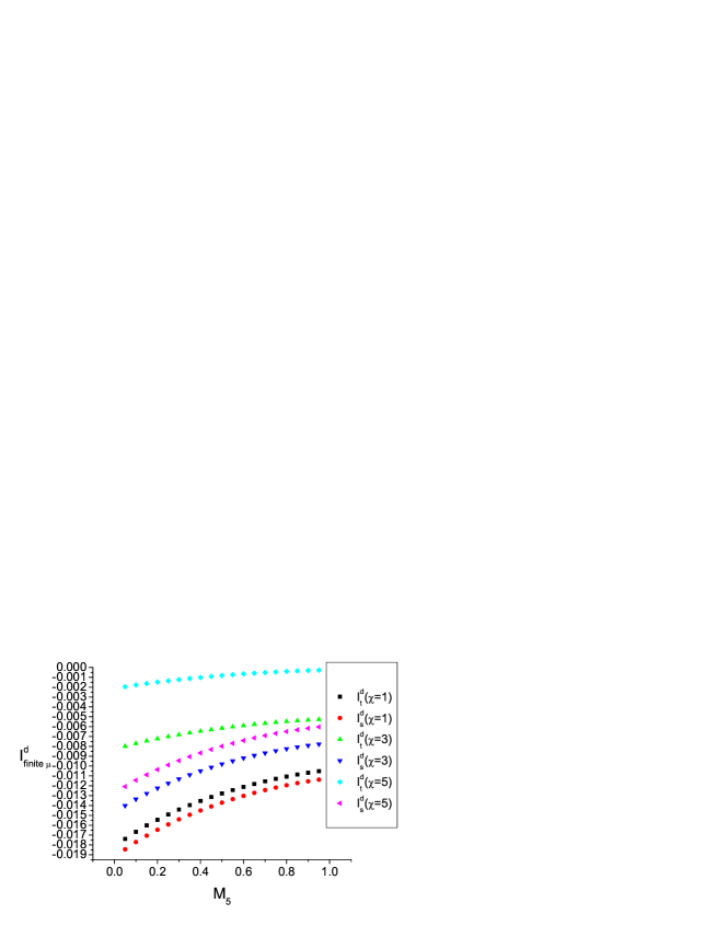
Figure 3: The values of $I^{d}_{\rm finite,\mu}$ as a function of $M_{5}$ for three values of anisotropy $\chi=1,3,5$ at $\kappa_{s}=1.0$, $\kappa_{t}=\chi\kappa_{s}$.

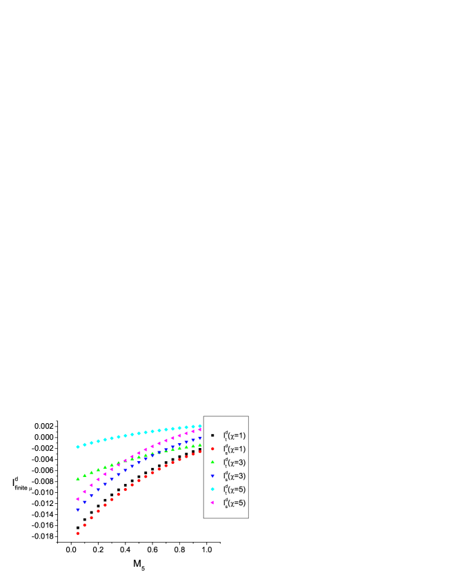
Figure 4: Same as in Fig. 3 but with $\kappa_{s}=0.5$.

For the massless case, the finite part of the half-circle diagram contribution, i.e. $I^{d}_{\rm finite,\mu}$, are calculated using numerical integration when the parameters of the theory are fixed. In Fig. 3 and Fig. 4 we have plotted the values of $I^{d}_{\rm finite,\mu}$ as a function of the parameter $M_{5}$ for three values of the anisotropy ($\chi=1,3,5$) and two values of $\kappa_{s}$ ($\kappa_{s}=1.0,0.5$). Since $I^{d}_{\rm finite,\mu}$ always corresponds to the massless case, we have set $\kappa_{t}=\chi\kappa_{s}$ in these plots. The infra-red divergent contribution from the half-circle diagram can be obtained from Eq. (86) once a infra-red scale is given.

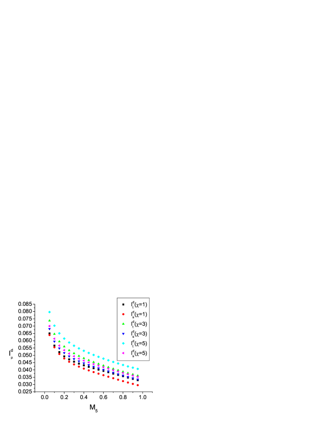
Figure 5: The values of $I^{d}_{\mu}(m)$ as a function of $M_{5}$ for three values of anisotropy: $\chi=1,3,5$ at current quark mass $m=0.3$. The parameter $\kappa_{s}=1.0$ and the values of $\kappa_{t}$ are adjusted accordingly, as discussed in Sec. 3.

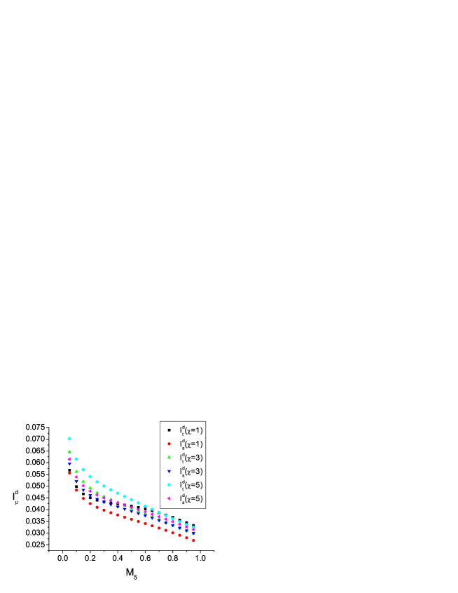
Figure 6: Same as in Fig. 5 with $\kappa_{s}=0.5$ and $m=0.3$.

For the massive case, one needs the values of $I^{d}_{\mu}(m)$ which is obtained by numerically integrating Eq. (56). The values of $I^{d}_{\mu}(m)$ are shown in Fig. 5 through Fig. 8. Similar to the massless case, the corresponding values of $I^{d}_{\mu}(m)$ are plotted as functions of $M_{5}$ for three values of anisotropy: $\chi=1,3,5$ and two values of $\kappa_{s}$ ($\kappa_{s}=1.0,0.5$).

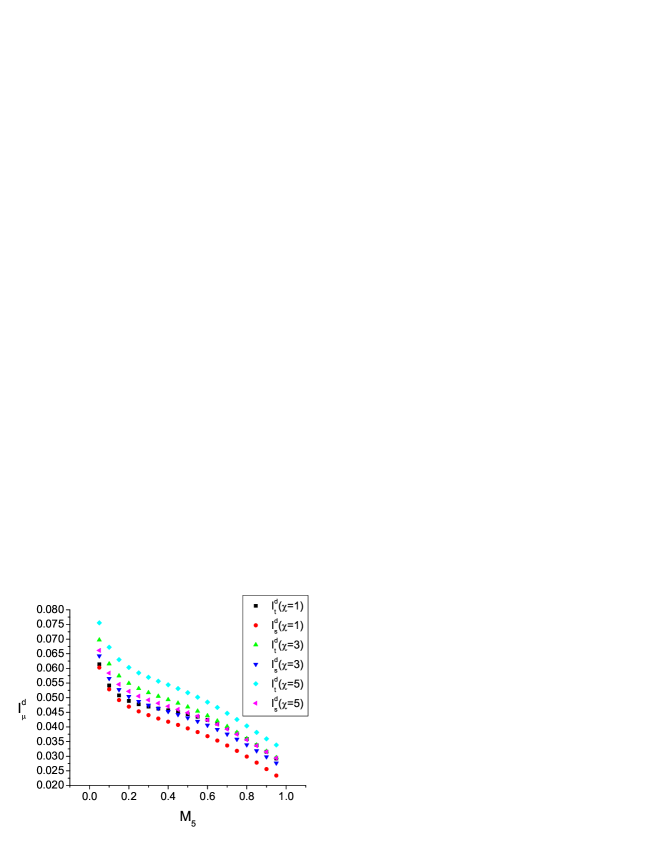
Figure 7: Same as Fig. 5 with current quark mass parameter $m=0.5$ and $\kappa_{s}=1.0$.

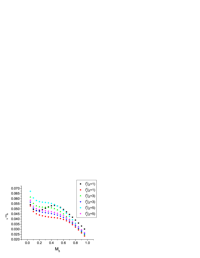
Figure 8: Same as Fig. 5 with current quark mass parameter $m=0.5$ and $\kappa_{s}=0.5$.

5.2 Mass renormalization for the domain wall fermion

For the mass renormalization factor given by Eq. (52), we obtain:

$$\tilde{Z}_{m}=1+g^{2}(M^{d}_{\rm tad}+M^{d}_{\rm log}+M^{d}_{\rm finite})\;,$$ (63)

for the massless case and for the massive case we have:

$$\tilde{Z}_{m}=1+g^{2}(M^{d}_{\rm tad}+M^{d})\;.$$ (64)

For the tadpole contribution $M^{d}_{\rm tad}$, using notation (55) and setting $\kappa_{s}=1.0$, we have evaluated the tadpole contribution $M^{0}_{\rm tad}$ for three values of anisotropy and the results are listed in Table 2.

Table 2: Values of $M^{0}_{\rm tad}$ for $\chi=1$, $3$, $5$ and $m=0$, $0.3$, $0.5$. The values listed here correspond to those at $\kappa_{s}=1$, $M_{5}=0.5$ and the values of $\kappa_{t}$ are tuned accordingly.

	$\chi=1$	$\chi=3$	$\chi=5$
$m=0.0$	$-0.357099$	$-0.409400$	$-0.409156$
$m=0.3$	$-0.355505$	$-0.408316$	$-0.408381$
$m=0.5$	$-0.352263$	$-0.406204$	$-0.406878$

The values of $M^{0}_{\rm tad}$ listed in Table 2 are obtained at: $\kappa_{s}=1$, $M_{5}=0.5$ with the values of $\kappa_{t}$ being tuned accordingly.

For the half-circle contributions in the massless case, values of $M^{d}_{\rm finite}$ are presented in Fig. 9 and Fig. 10

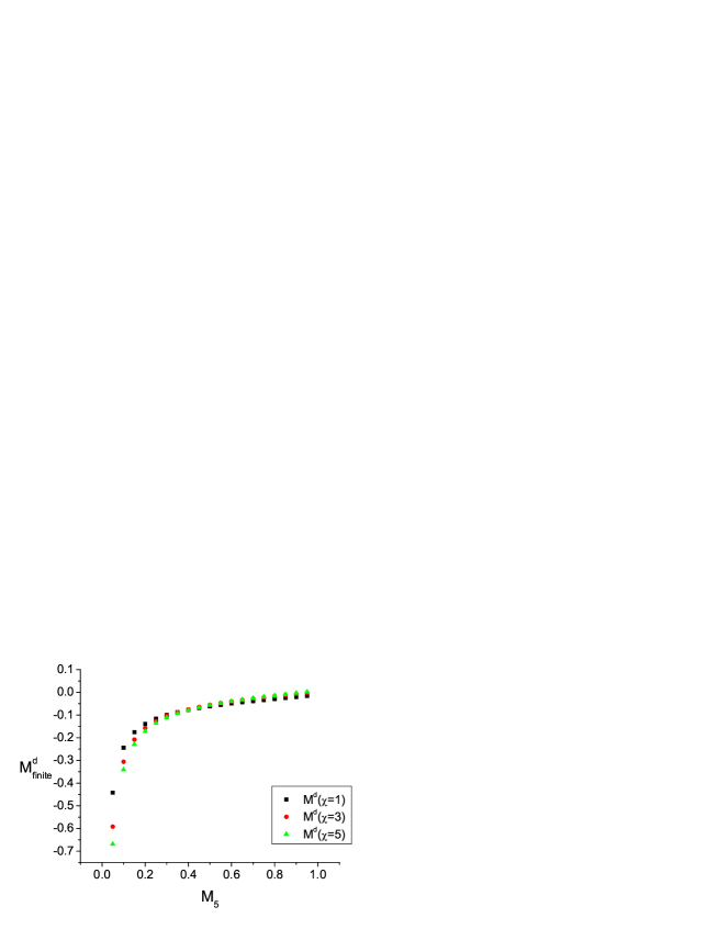
Figure 9: The values of $M^{d}_{\rm finite}$ as a function of $M_{5}$ are shown for $\chi=1$, $3$ and $5$. Other parameters are: $\kappa_{s}=1$, $\kappa_{t}=\chi\kappa_{s}$, $m=0$.

where we have shown the values of $M^{d}_{\rm finite}$ for $\kappa_{s}=1.0$ and $\kappa_{s}=0.5$, respectively. In each figure, three values of the anisotropy, namely $\chi=1,3,5$, are taken to evaluate $M^{d}_{\rm finite}$ as a function of $M_{5}$ which is taken to vary between zero and unity.

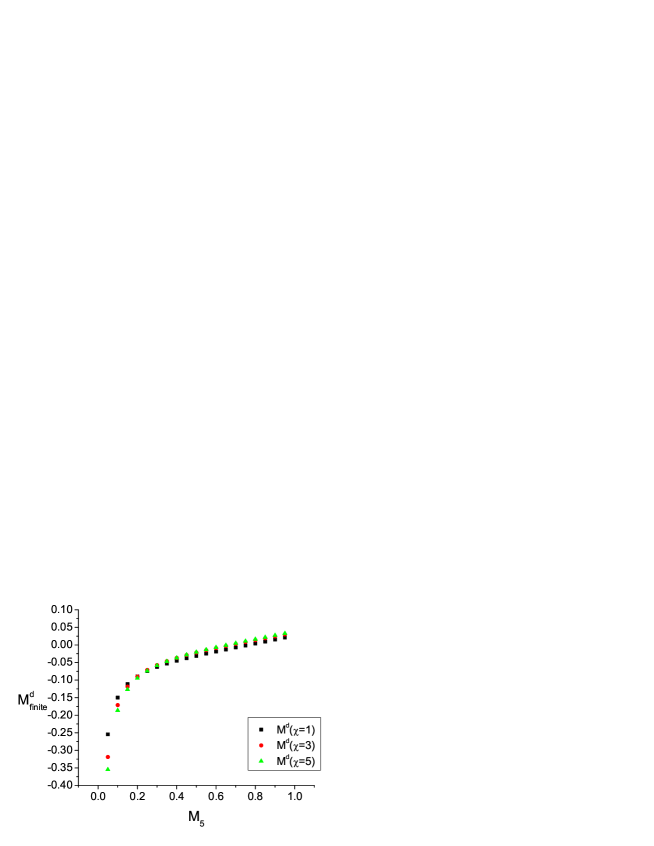
Figure 10: Same as Fig. 9 except that $\kappa_{s}=0.5$.

For the massive case, we evaluate $M^{d}(m)$ directly by numerical integration.

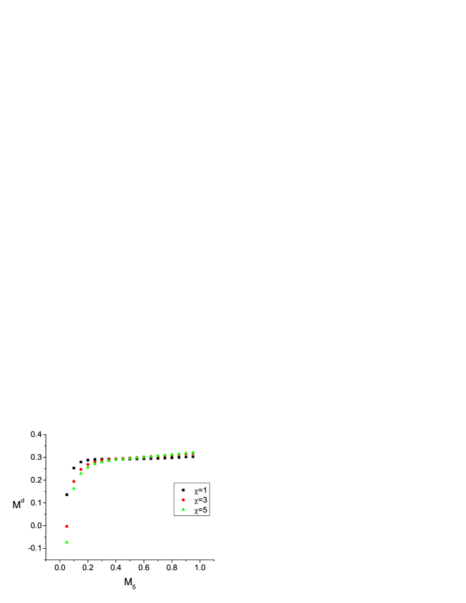
Figure 11: The value of $M^{d}$ as a function of $M_{5}$ is shown for $\chi=1$, $3$ and $5$. Other parameters are: $\kappa_{s}=1$, $m=0.3$.

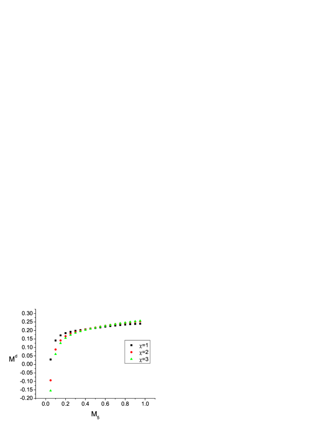
Figure 12: The value of $M^{d}$ as a function of $M_{5}$ is shown for $\chi=1$, $3$ and $5$. Other parameters are: $\kappa_{s}=1$, $m=0.5$.

In Fig. 11 and Fig. 12, we have shown the values of $M^{d}(m)$ as a function of $M_{5}$ at $m=0.3$ and $m=0.5$, respectively. We have also taken three values for the anisotropy parameter in each case.

5.3 Mass shift for the parameter $M_{5}$ in mean-field theory

At the tree level, it is known that the domain wall fermion preserves chiral properties only when the parameter $M_{5}$ is tuned to the right interval ( $0<M_{5}<1$ for free domain wall fermion). Since this parameter enters the action via a five-dimensional mass term, one expects that it receives substantial additive renormalization. At one-loop level, it is important to check that, after renormalization effects are taken into account, whether this so-called “chiral window” for $M_{5}$ remains there or not. In the case of isotropic lattices, it has been shown that the window remains in perturbation theory and one expects chiral properties of the fermion as long as $M_{5}$ lies in the right interval. We wish to check this point for the anisotropic lattices.

In perturbation theory, as expected, the main contribution for the shift of the parameter $M_{5}$ comes from the tadpole diagram. To simplify the analysis, we will only discuss the shift of $M_{5}$ due to tadpole diagrams. Within this approximation, one finds that the parameter $M_{5}$ is replaced by:

$$\tilde{M_{5}}=M_{5}-(\kappa_{t}(1-U_{t})+3\kappa_{s}(1-U_{s}))\equiv M_{5}-\delta(M_{5})\;,$$ (65)

where the tadpole parameters $U_{t}$ and $U_{s}$ are given by:

$$U_{t} = U_{0}=1-g^{2}C_{F}\frac{1}{2}\int_{-\pi}^{\pi}\frac{d^{4}l}{(2\pi)^{4}}\frac{1}{(\chi^{2}\hat{l}^{2}_{0}+\sum_{j}\hat{l}^{2}_{j})^{2}}(\hat{l}^{2}_{0}\chi+\frac{f^{00}}{f_{D}})\;,$$

$$U_{s} = U_{i}=1-g^{2}C_{F}\frac{1}{2}\int_{-\pi}^{\pi}\frac{d^{4}l}{(2\pi)^{4}}\frac{1}{(\chi^{2}\hat{l}^{2}_{0}+\sum_{j}\hat{l}^{2}_{j})^{2}}(\hat{l}^{2}_{i}\chi+\frac{f^{ii}}{f_{D}})\;,$$ (66)

here $g^{2}$ and $\chi$ are the “boosted” coupling and the “boosted” anisotropy [29] which are defined as:

$$g^{2}=\frac{2N_{c}}{\beta_{0}}U^{3}_{s}U_{t}\;,\;\;\chi=\chi_{0}\frac{U_{s}}{U_{t}}\;.$$ (67)

Eq. (65) suggests that in perturbation the chiral window remains but it is shifted.

We will only show results at zero current quark mass $m=0$ in which case we have: $\kappa_{t}/\kappa_{s}=\chi$. To get a feeling how large the shift in the parameter $M_{5}$ can get, we take a particular value of $\beta_{0}$. At first, the values of $U_{t}$ and $U_{s}$ are set as $U_{t}=U_{s}=1$. By making use of the formula (67), the values of $g^{2}$ and $\chi$ are obtained and can be substituted into formula (5.3) to obtain a new set of values for $U_{t}$ and $U_{s}$. The above procedure is repeated iteratively until the values of $U_{t}$ and $U_{s}$ become stable. The ultimate values for $U_{t}$ and $U_{s}$ in perturbation theory and the corresponding shift in $M_{5}$ thus obtained are listed in Table 3 for $\beta_{0}=3.0$

Table 3: The values of tadpole improvement parameters $U_{t}$, $U_{s}$ and corresponding values for $\delta M_{5}$ as evaluated from Eq. (65) at $\chi_{0}=1$ to $\chi_{0}=5$. The bare gauge coupling is $\beta_{0}=3.0$ and the parameter $\kappa_{s}=1$.

	$\chi_{0}=1$	$\chi_{0}=2$	$\chi_{0}=3$	$\chi_{0}=4$	$\chi_{0}=5$
$U_{t}$	$0.889580$	$0.956099$	$0.977525$	$0.986559$	$0.991122$
$U_{s}$	$0.891130$	$0.861399$	$0.851613$	$0.847194$	$0.844862$
$\delta(M_{5})$	$0.437222$	$0.494908$	$0.503901$	$0.504587$	$0.503253$

at five different values of $\chi_{0}$.

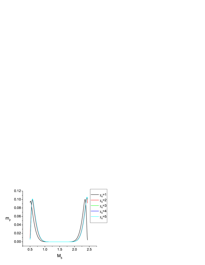
Figure 13: The effective mass of the chiral mode, $m_{F}$, as a function of the parameter $M_{5}$ at $m=0.0$, $L_{s}=10$. Five curves with different colors correspond to different values of $\chi_{0}$. The values of $U_{t}$ and $U_{s}$ are taken to be those in Table 3 at $\beta_{0}=3.0$.

Another way to investigate the renormalization of parameter $M_{5}$ is to use mean-field approximation. In this case, the domain wall fermion action is rewritten as:

$$[S_{\rm MF}]_{s,s^{\prime}} = \left(-\tilde{b}(p)+i\sum_{\mu}\kappa_{\mu}U_{\mu}\gamma_{\mu}\sin p_{\mu}\right)\delta_{s,s^{\prime}}$$ (68)

$$+ P_{R}\delta_{s+1,s^{\prime}}+P_{L}\delta_{s-1,s^{\prime}}\;,$$

where $U_{\mu}$ are pure numbers and $\tilde{b}(p)$ is defined as:

$$\tilde{b}(p) = 1-M_{5}+\sum_{\mu}\kappa_{\mu}(1-U_{\mu}\cos p_{\mu})\;.$$ (69)

Following similar calculations as for the free domain wall propagator, one can define an effective mass for the fermion in the mean-field approximation. We will denote this mass parameter as $m_{F}$.

In Fig. 13, we show the effective mass $m_{F}$ of the chiral mode as a function of the parameter $M_{5}$ for five values of $\chi_{0}$. For simplicity, we have set $\kappa_{s}=1$ in this figure and the extent in the fifth dimension is taken to be $L_{s}=10$. It is seen from the figure that, within a certain interval, the chiral window remains for all $\chi_{0}$. This has been checked in the case of isotropic lattice which roughly corresponds to the red curve in our figure. We see from the figure that this qualitative feature remains valid in the anisotropic lattice case for almost all values of anisotropy $\chi_{0}$. In fact the shape of the curves is quite insensitive to the value of $\chi_{0}$, as is seen from the figure. The size of the chiral window remains more or less unchanged but the starting and ending position is shifted. The results discussed above suggest that, as long as the parameter $M_{5}$ is tuned to the right interval, massless chiral modes are stable against perturbative quantum fluctuations. This result also serves as a guidance for the choice of the parameters in our future numerical simulations.

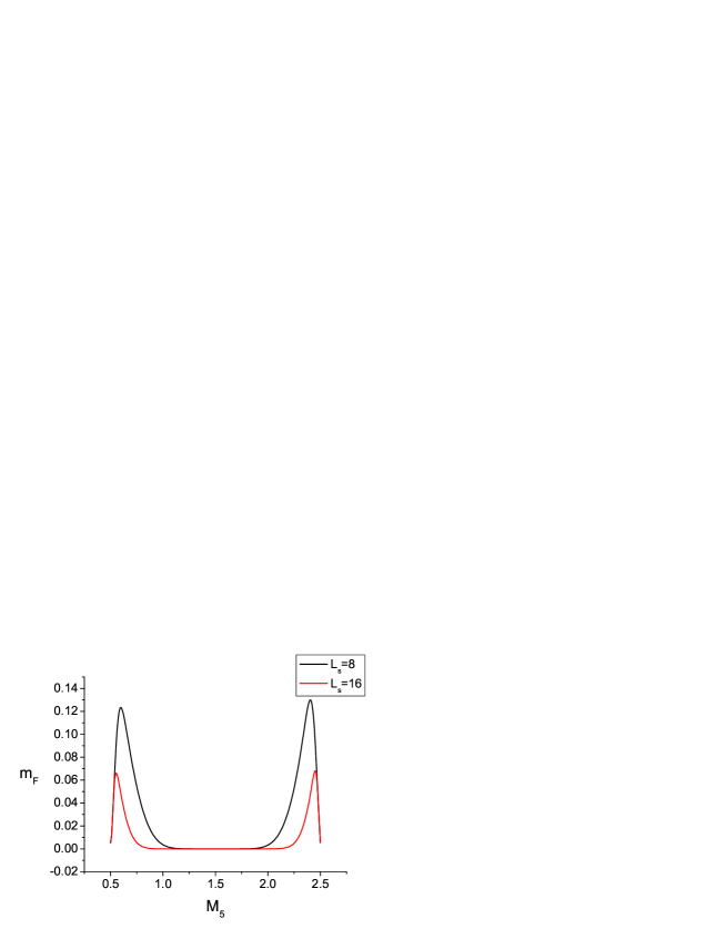
Figure 14: The effective mass $m_{F}$ of the chiral mode as a function of $M_{5}$ for two different values of $L_{s}$. The red and black curve corresponds to $L_{s}=16$ and $L_{s}=8$, respectively. Other parameters are the same as those in Fig. 13.

We have also investigated the dependence of the chiral window on the size of the fifth dimension $L_{s}$. In Fig. 14, we have plotted the effective mass of the chiral mode as a function of $M_{5}$ at two different values of $L_{s}$. The anisotropy parameter is set to $\chi_{0}=5$ while all other parameters are kept the same as those in Fig. 13. It is seen from the figure that the chiral window for the smaller lattice ($L_{s}=8$) becomes narrower than that of the larger lattice ($L_{s}=16$), as expected.

6 Conclusions

In this paper we have studied the domain wall fermions on anisotropic four-dimensional lattices. We have analyzed the free domain wall fermions, showing that the hopping parameters have to be tuned according to the current quark mass parameter in order to restore the correct dispersion relation for the chiral mode of the domain wall fermion. Using lattice perturbation theory, the domain wall fermion self-energy is calculated to one-loop order. We obtained the wave-function renormalization constant $\tilde{Z}_{\mu}$ and the mass renormalization constant $\tilde{Z}_{m}$ for the chiral mode. It is also verified that the chiral property of the fermion remains when quantum corrections are considered. We have also estimated the range for the parameter $M_{5}$ in order to maintain a chiral mode.

From our study, it seems that domain wall fermion on anisotropic lattices is applicable in practical Monte Carlo simulations. The only parameter that has to be tuned is the hopping parameter $\kappa_{t}$ when other parameters are given. The tuning of this parameter can be done either perturbatively or non-perturbatively. The non-perturbative tuning requires the measurement of physical hadron dispersion relations or quark dispersion relations by Monte Carlo simulations. An exploratory numerical study is now under way and we hope to come up with some results in the future [20]. Compared with similar situations for the Wilson fermions, anisotropic lattice domain wall fermion appears to be less complicated since there is no need to add clover terms (or other dimension five operators) due to better chiral properties. Of course, this conclusion relies on the fact that the residual mass effects due to the finite extent of the fifth dimension to be small. We have tried to estimate this effect with mean-field approximation but this issue definitely should be checked further in future numerical studies.

It should be straightforward to generalize the results we obtained in this paper to the overlap fermions on anisotropic lattices. Another topic that is worth studying is the renormalization factors for quark bilinear operators. The study of these problems are now under investigation. To summarize, we anticipate the anisotropic domain wall fermions to be helpful in the study of the heavy-light hadronic systems, exotic hadrons (hybrid) with light quarks and light hadron-hadron scattering processes and we hope to come up with some exploratory numerical results in the future [20].

Appendix A Dispersion relation of free domain wall fermions

In this appendix, we briefly outline the derivation of the dispersion relation for the free domain wall fermion on anisotropic lattices. The dispersion relation is such that the four-momentum $p=(iE_{\mathbf{p}},{\mathbf{p}})$ is a zero of the function:

$$\Delta=(1+mm_{r})^{2}be^{2\alpha_{G}}-(1-m^{2})(1-m_{r}^{2})e^{\alpha_{G}}-(m+m_{r})^{2}b\;.$$ (70)

In principle, the parameter $m_{r}=e^{-\alpha_{G}L_{s}}$ also depends on the four-momentum. For the moment, we assume that the extension in the fifth dimension is large enough such that we can ignore the momentum dependence of $m_{r}$ in the study of the dispersion relation. This amounts to taking $m_{r}=e^{-\alpha_{G}(0)L_{s}}$. If we denotes:

$$m_{1}=(1+mm_{r})^{2}\;,\;\;m_{2}=(1-m^{2})(1-m^{2}_{r})\;,m_{3}=(m+m_{r})^{2}\;.$$ (71)

Then, the equation for the pole yields:

$$-\tilde{p}^{2}=M_{1}\left[(1+b^{2}+\tilde{p}^{2})^{2}-4b^{2}\right]\;,$$ (72)

where $M_{1}=m_{1}m_{3}/m_{2}^{2}$. The complete dispersion relation turns out to be quite complicated. But if the lattice three-momentum $|{\mathbf{p}}|\ll 1$, we obtain:

$$E_{\mathbf{p}}=E_{0}+{{\mathbf{p}}^{2}\over 2M_{kin}}+O({\mathbf{p}}^{4})\;,$$ (73)

where $E_{0}$ will be identified as the pole mass of the quark: $E_{0}=m_{Q}$ and $M_{kin}$ is the so-called kinetic mass. After some calculations, the equation satisfied by $E_{0}=m_{Q}$ is found to be:

$$A\cosh^{2}E_{0}+B\cosh E_{0}+C=0$$ (74)

where

$$A = \kappa_{t}^{2}-4\kappa_{t}^{2}\left[(b(0)+\kappa_{t})^{2}-1\right]M_{1}$$

$$B = 4(b(0)+\kappa_{t})\kappa_{t}\left[(b(0)+\kappa_{t})^{2}+\kappa_{t}^{2}-1\right]M_{1}$$

$$C = -\kappa_{t}^{2}-\left[(b(0)+\kappa_{t})^{4}+2(b(0)+\kappa_{t})^{2}(\kappa_{t}^{2}-1)+(\kappa_{t}^{2}+1)^{2}\right]M_{1}$$ (75)

We can also find out the kinetic mass term with the result:

$${1\over 2M_{kin}}=\frac{dE}{d\vec{p}^{2}}\left|{}_{\vec{p}=0}=\frac{A_{1}\cosh^{2}E_{0}+B_{1}\cosh E_{0}+C_{1}}{(2A\cosh E_{0}+B)\sinh E_{0}}\right.$$ (76)

where

$$A_{1} = 4(b(0)+\kappa_{t})\kappa_{t}^{2}\kappa_{s}M_{1}$$

$$B_{1} = -2\left[3(b(0)+\kappa_{t})^{2}+2(b(0)+\kappa_{t})\kappa_{s}+\kappa_{t}^{2}-1\right]\kappa_{t}\kappa_{s}M_{1}$$

$$C_{1} = \kappa_{s}^{2}+2\kappa_{s}\left[(b(0)+\kappa_{t})\left((b(0)+\kappa_{t})^{2}+\kappa_{t}^{2}-1\right)\right.$$ (77)

$$+ \left.\kappa_{s}\left((b(0)+\kappa_{t})^{2}+\kappa_{t}^{2}+1\right)\right]M_{1}$$

In order to have the usual energy-momentum dispersion relation, one imposes the condition: $M_{kin}=m_{Q}$ which yields the relationship between $\chi$ and $\kappa_{t},\kappa_{s}$ as (restoring the lattice spacing explicitly):

$$\chi^{2}=\frac{(2A\cosh E_{0}+B)\sinh E_{0}}{2(A_{1}\cosh^{2}E_{0}+B_{1}\cosh E_{0}+C_{1})E_{0}}\;,$$ (78)

where $E_{0}=m_{Q}$ is obtained by solving Eq. (74). Eq. (74) and Eq. (78) thus establish the relation among the pole mass $m_{Q}$, anisotropy $\chi$ and the other bare parameters of the theory for free domain wall fermions on anisotropic lattices.

In the above discussions, we have neglected the momentum dependence of $m_{r}=e^{-\alpha_{G}(p)L_{s}}$. If we keep this momentum dependence, the pole position can be solved numerically. For any given set of parameters, we start with the choice $m_{r}=e^{-\alpha_{G}(0)L_{s}}$ and solve for $m_{Q}$ in Eq. (74). Then the obtained value of $E_{0}=m_{Q}$ is substituted into $m_{r}=e^{-\alpha_{G}(iE_{0},0,0,0)L_{s}}$ and a new value of $E_{0}$ is thus obtained by solving Eq. (74) again. This procedure can be iterated until a stable set of values for $m_{Q}$ and $m_{r}=e^{-\alpha_{G}(im_{Q},0,0,0)L_{s}}$ is obtained. The figures in the main text are obtained using this method for a given $L_{s}=8$.

Appendix B Some Explicit formulae for loop integrals

In this appendix, we list the explicit expressions for various loop integrals which enters the fermion self-energy discussed in section 4.2.

First, the tadpole contributions $I_{\rm tad,\mu}$ and $M_{\rm tad}$ are given by:

$$I_{\rm tad,\mu}(s,s^{\prime}) = -g^{2}C_{F}\frac{1}{2}\int_{-\pi}^{\pi}\frac{d^{4}l}{(2\pi)^{4}}\frac{1}{(\chi^{2}\hat{l}^{2}_{0}+\sum_{j}\hat{l}^{2}_{j})^{2}}(\hat{l}^{2}_{\mu}\chi+\frac{f^{\mu\mu}}{f_{D}})\delta_{s,s^{\prime}}\;,$$

$$M_{\rm tad}(s,s^{\prime}) = -g^{2}C_{F}\frac{1}{2}\int_{-\pi}^{\pi}\frac{d^{4}l}{(2\pi)^{4}}\sum_{\mu}\frac{\kappa_{\mu}}{(\chi^{2}\hat{l}^{2}_{0}+\sum_{j}\hat{l}^{2}_{j})^{2}}(\hat{l}^{2}_{\mu}\chi+\frac{f^{\mu\mu}}{f_{D}})\delta_{s,s^{\prime}}\;.$$ (79)

Note that these tadpole contributions are diagonal in the fifth dimension. It is also noted that $I_{\rm tad,\mu}$ and $M_{\rm tad}$ are independent of the current quark mass parameter $m$ explicitly.

Now comes the formulae for the half-circle diagrams. In massive case, we have:

$$[I_{\mu}^{+}(m)]_{s,s^{\prime}} = g^{2}C_{F}\int\frac{d^{4}l}{(2\pi)^{4}}\Biggl{\{}\Biggl{[}\frac{1}{2}\kappa_{\mu}\left(\cos l_{\mu}(W^{-}G_{R}+W^{+}G_{L})(s,s^{\prime})\right.$$ (80)

$$+ \left.\kappa_{\mu}\sin^{2}l_{\mu}(G_{L}+G_{R})(s,s^{\prime})\right)\Biggr{]}\frac{\chi\hat{l}^{2}_{\mu}+\frac{f^{\mu\mu}(l)}{f_{D}(l)}}{(\chi^{2}\hat{l}^{2}_{0}+\sum_{j}\hat{l}^{2}_{j})^{2}}$$

$$+ \Biggl{[}\left(\frac{1}{2}\kappa_{\mu}(W^{-}G_{R}+W^{+}G_{L})-2\kappa^{2}_{\mu}\cos^{2}l_{\mu}/2G_{L}\right)(s,s^{\prime})\times$$

$$\left(\frac{4(\chi^{2})^{\delta_{\mu 0}}}{\chi^{2}\hat{l}^{2}_{0}+\sum_{j}\hat{l}^{2}_{j}}(\chi\hat{l}^{2}_{\mu}+\frac{f^{\mu\mu}(l)}{f_{D}(l)})-2\chi-\frac{f^{\mu}_{\mu}(l)}{f_{D}(l)}+\frac{f^{D}_{\mu}(l)f^{\mu\mu}(l)}{f^{2}_{D}(l)}\right)$$

$$- 2\chi\kappa^{2}_{\mu}\left(\sin^{2}l_{\mu}/2G_{R}+\cos^{2}l_{\mu}/2G_{L}\right)(s,s^{\prime})$$

$$+ \sum_{\nu}\kappa^{2}_{\nu}\left(\sin^{2}l_{\nu}/2G_{R}+\cos^{2}l_{\nu}/2G_{L}\right)(s,s^{\prime})$$

$$\times \left(\frac{4(\chi^{2})^{\delta_{\mu 0}}}{\chi^{2}\hat{l}^{2}_{0}+\sum_{j}\hat{l}^{2}_{j}}(\chi\hat{l}^{2}_{\nu}+\frac{f^{\nu\nu}(l)}{f_{D}(l)})-\frac{f^{\nu}_{\mu}(l)}{f_{D}(l)}+\frac{f^{D}_{\mu}(l)f^{\nu\nu}(l)}{f^{2}_{D}(l)}\right)\Biggr{]}$$

$$\times \frac{\sin^{2}l_{\mu}}{(\chi^{2}\hat{l}^{2}_{0}+\sum_{j}\hat{l}^{2}_{j})^{2}}\Biggr{\}}$$

$$[I_{\mu}^{-}(m)]_{s,s^{\prime}} = g^{2}C_{F}\int\frac{d^{4}l}{(2\pi)^{4}}\Biggl{\{}\Biggl{[}\frac{1}{2}\kappa_{\mu}\left(\cos l_{\mu}(W^{-}G_{R}+W^{+}G_{L})(s,s^{\prime})\right.$$ (81)

$$+ \left.\kappa_{\mu}\sin^{2}l_{\mu}(G_{L}+G_{R})(s,s^{\prime})\right)\Biggr{]}\frac{\chi\hat{l}^{2}_{\mu}+\frac{f^{\mu\mu}(l)}{f_{D}(l)}}{(\chi^{2}\hat{l}^{2}_{0}+\sum_{j}\hat{l}^{2}_{j})^{2}}$$

$$+ \Biggl{[}\left(\frac{1}{2}\kappa_{\mu}(W^{-}G_{R}+W^{+}G_{L})-2\kappa^{2}_{\mu}\cos^{2}l_{\mu}/2G_{R}\right)(s,s^{\prime})$$

$$\times \left(\frac{4(\chi^{2})^{\delta_{\mu 0}}}{\chi^{2}\hat{l}^{2}_{0}+\sum_{j}\hat{l}^{2}_{j}}(\chi\hat{l}^{2}_{\mu}+\frac{f^{\mu\mu}(l)}{f_{D}(l)})-2\chi-\frac{f^{\mu}_{\mu}(l)}{f_{D}(l)}+\frac{f^{D}_{\mu}(l)f^{\mu\mu}(l)}{f^{2}_{D}(l)}\right)$$

$$- 2\chi\kappa^{2}_{\mu}\left(\sin^{2}l_{\mu}/2G_{L}+\cos^{2}l_{\mu}/2G_{R}\right)(s,s^{\prime})$$

$$+ \sum_{\nu}\kappa^{2}_{\nu}\left(\sin^{2}l_{\nu}/2G_{L}+\cos^{2}l_{\nu}/2G_{R}\right)(s,s^{\prime})$$

$$\times \left(\frac{4(\chi^{2})^{\delta_{\mu 0}}}{\chi^{2}\hat{l}^{2}_{0}+\sum_{j}\hat{l}^{2}_{j}}(\chi\hat{l}^{2}_{\nu}+\frac{f^{\nu\nu}(l)}{f_{D}(l)})-\frac{f^{\nu}_{\mu}(l)}{f_{D}(l)}+\frac{f^{D}_{\mu}(l)f^{\nu\nu}(l)}{f^{2}_{D}(l)}\right)\Biggr{]}$$

$$\times \frac{\sin^{2}l_{\mu}}{(\chi^{2}\hat{l}^{2}_{0}+\sum_{j}\hat{l}^{2}_{j})^{2}}\Biggr{\}}$$

$$[M^{+}(m)]_{s,s^{\prime}} = g^{2}C_{F}\int\frac{d^{4}l}{(2\pi)^{4}}\sum_{\mu}\kappa^{2}_{\mu}\Biggl{[}\cos^{2}l_{\mu}/2(W^{+}G_{L})(s,s^{\prime})$$ (82)

$$- \sin^{2}l_{\mu}/2(W^{-}G_{R})(s,s^{\prime})+\frac{1}{2}\kappa_{\mu}\sin^{2}l_{\mu}(G_{L}+G_{R})(s,s^{\prime})\Biggr{]}$$

$$\times \frac{\chi\hat{l}^{2}_{\mu}+\frac{f^{\mu\mu}(l)}{f_{D}(l)}}{(\chi^{2}\hat{l}^{2}_{0}+\sum_{j}\hat{l}^{2}_{j})^{2}}$$

$$[M^{-}(m)]_{s,s^{\prime}} = g^{2}C_{F}\int\frac{d^{4}l}{(2\pi)^{4}}\sum_{\mu}\kappa^{2}_{\mu}\Biggl{[}\cos^{2}l_{\mu}/2(W^{-}G_{R})(s,s^{\prime})$$ (83)

$$- \sin^{2}l_{\mu}/2(W^{+}G_{L})(s,s^{\prime})+\frac{1}{2}\kappa_{\mu}\sin^{2}l_{\mu}(G_{L}+G_{R})(s,s^{\prime})\Biggr{]}$$

$$\times \frac{\chi\hat{l}^{2}_{\mu}+\frac{f^{\mu\mu}(l)}{f_{D}(l)}}{(\chi^{2}\hat{l}^{2}_{0}+\sum_{j}\hat{l}^{2}_{j})^{2}}\;,$$

where we have used the following notations:

$$f^{\nu}_{\mu}(l)=-\frac{\partial f^{\mu\mu}(p-l)}{\sin l_{\mu}\partial p_{\mu}}\Bigg{|}_{p=0},\quad f^{D}_{\mu}(l)=-\frac{\partial f_{D}(p-l)}{\sin l_{\mu}\partial p_{\mu}}\Bigg{|}_{p=0}\;.$$ (84)

It’s easy to verify that $M^{\pm}(m)$ is proportional to $m_{P}=(1-b^{2}(0))m$. Thus, we may define:

$$[M^{\pm}(m)]_{s,s^{\prime}}=(1-b^{2}(0))m[M_{0}^{\pm}(m)]_{s,s^{\prime}}$$ (85)

In massless case:

$$I^{\pm}_{\log,\mu}(s,s^{\prime}) = \frac{1}{16\pi^{2}}g^{2}C_{F}(C_{\pm})_{s,s^{\prime}}\Biggl{(}\ln(\pi^{2})+1-\ln(\tilde{p}^{2})+\ln{\kappa^{2}_{s}}\Biggr{)}$$ (86)

$$I_{\rm finite,\mu}^{+}(s,s^{\prime}) = [I_{\mu}^{+}(m=0)]_{s,s^{\prime}}-g^{2}C_{F}(C_{+})_{s,s^{\prime}}$$ (87)

$$\times \int\frac{d^{4}l}{(2\pi)^{4}}\frac{4\chi(\chi^{2})^{\delta_{\mu 0}}l^{2}_{\mu}\theta(\pi^{2}-(\chi^{2}l^{2}_{0}+\sum_{j}l^{2}_{j}))}{(\chi^{2}l^{2}_{0}+\sum_{j}l^{2}_{j})^{3}}$$

$$I_{\rm finite,\mu}^{-}(s,s^{\prime}) = [I_{\mu}^{-}(m=0)]_{s,s^{\prime}}-g^{2}C_{F}(C_{-})_{s,s^{\prime}}$$ (88)

$$\times \int\frac{d^{4}l}{(2\pi)^{4}}\frac{4\chi(\chi^{2})^{\delta_{\mu 0}}l^{2}_{\mu}\theta(\pi^{2}-(\chi^{2}l^{2}_{0}+\sum_{j}l^{2}_{j}))}{(\chi^{2}l^{2}_{0}+\sum_{j}l^{2}_{j})^{3}}$$

$$M^{\pm}_{\log}(s,s^{\prime}) = \frac{1}{4\pi^{2}}g^{2}C_{F}(C^{M}_{\pm})_{s,s^{\prime}}\left(\ln(\pi^{2})+1-\ln(\tilde{p}^{2})+\ln{\kappa^{2}_{s}}\right)$$ (89)

$$M^{+}_{\rm finite}(s,s^{\prime}) = m_{P}\left\{[M_{0}^{+}(m=0)]_{s,s^{\prime}}\right.$$ (90)

$$- g^{2}C_{F}\left.\frac{(C^{M}_{+})_{s,s^{\prime}}}{m_{P}}\int\frac{d^{4}l}{(2\pi)^{4}}\frac{4\chi\theta(\pi^{2}-(\chi^{2}l^{2}_{0}+\sum_{j}l^{2}_{j}))}{(\chi^{2}l^{2}_{0}+\sum_{j}l^{2}_{j})^{2}}\right\}$$

$$M^{-}_{\rm finite}(s,s^{\prime}) = m_{P}\left\{[M_{0}^{-}(m=0)]_{s,s^{\prime}}\right.$$ (91)

$$- \left.g^{2}C_{F}\frac{(C^{M}_{-})_{s,s^{\prime}}}{m_{P}}\int\frac{d^{4}l}{(2\pi)^{4}}\frac{4\chi\theta(\pi^{2}-(\chi^{2}l^{2}_{0}+\sum_{j}l^{2}_{j}))}{(\chi^{2}l^{2}_{0}+\sum_{j}l^{2}_{j})^{2}}\right\}$$

where $(C^{M}_{\pm})_{s,s^{\prime}}$ are given by:

$$(C^{M}_{+})_{s,s^{\prime}} = (1-b^{2}(0))m\left[\delta_{s,L_{s}-1}e^{-\alpha_{0}s^{\prime}}\right.$$ (92)

$$+ \left.b(0)\left(\sum_{t}W^{+}(0)_{s,t}e^{-\alpha_{0}(L_{s}-1-t+s^{\prime})}\right)\right]\;,$$

$$(C^{M}_{-})_{s,s^{\prime}} = (1-b^{2}(0))m\left[\delta_{s,0}e^{-\alpha_{0}(L_{s}-1-s^{\prime})}\right.$$ (93)

$$+ \left.b(0)\left(\sum_{t}W^{-}(0)_{s,t}e^{-\alpha_{0}(L_{s}-1+t-s^{\prime})}\right)\right]\;.$$

References

- [1] D. Kaplan. Phys. Lett. B, 288:342, 1992.
- [2] Y. Shamir. Nucl. Phys. B, 406:90, 1993.
- [3] R. Narayanan and H. Neuberger. Phys. Rev. Lett., 71:3251, 1993.
- [4] R. Narayanan and H. Neuberger. Nucl. Phys. B, 412:574, 1994.
- [5] Herbert Neuberger. Phys. Rev. D, 57(9):5417–5433, May 1998.
- [6] H. Neuberger. Phys. Lett. B, 417:141, 1998.
- [7] C. Morningstar and M. Peardon. Phys. Rev. D, 60:034509, 1999.
- [8] C. Liu. Chinese Physics Letter, 18:187, 2001.
- [9] P. Chen. Phys. Rev. D, 64:034509, 2001.
- [10] M. Okamoto et al. Phys. Rev. D, 65:094508, 2002.
- [11] A. Juettner and J. Rolf. Phys. Lett. B, 560:59, 2003.
- [12] R. Lewis, N. Mathur, and R.M. Woloshyn. Phys. Rev. D, 64:094509, 2001.
- [13] C. Liu, J. Zhang, Y. Chen, and J.P. Ma. Nucl. Phys. B, 624:360, 2002.
- [14] G. Meng, C. Miao, X. Du, and C. Liu. hep-lat/0309048, 2003.
- [15] C. Miao, X. Du, G. Meng, and C. Liu. hep-lat/0403028, 2004.
- [16] X. Du, C. Miao, G. Meng, and C. Liu. hep-lat/0404017, 2004.
- [17] HueyWen Lin, Shigemi Ohta, and Norikazu Yamada. PoS LAT2005, page 96, 2005.
- [18] Silas R. Beane, Paulo F. Bedaque, Kostas Orginos, and Martin J. Savage. Phys. Rev. D, 73:054503, 2006.
- [19] C. Morningstar and M. Peardon. Phys. Rev. D, 56:4043, 1997.
- [20] C. Liu et al. work in progress.
- [21] Y. Kikukawa, H. Neuberger, and A. Yamada. Nucl. Phys. B, 526:572, 1998.
- [22] S. Aoki and Y. Taniguchi. Phys. Rev. D, 59:054510, 1999.
- [23] C. Liu. Communications in Theoretical Physics, 35:288, 2001.
- [24] C. Liu. In Proceedings of International Workshop on Nonperturbative Methods and Lattice QCD, page 57. World Scientific, Singapore, 2001.
- [25] C. Liu and J. P. Ma. In Proceedings of International Workshop on Nonperturbative Methods and Lattice QCD, page 65. World Scientific, Singapore, 2001.
- [26] C. Liu. Nucl. Phys. (Proc. Suppl.) B, 94:255, 2001.
- [27] Y. Shamir. Phys. Lett. B, 305:357, 1993.
- [28] Stefan Groote and Junko Shigemitsu. Phys. Rev. D, 62:014508, 2000.
- [29] I.T. Drummond, A. Hart, R.R. Horgan, and L.C. Storoni. Phys. Rev. D, 66:094509, 2002.