Flavor Twisted Boundary Conditions and Isovector Form Factors

Abstract

We use vector flavor symmetry to relate form factors of isospin changing operators to isovector form factors. Flavor twisted boundary conditions in lattice QCD thus allow isovector form factors of twist-two operators, e.g, to be computed at continuous values of the momentum transfer. These twisted boundary conditions, moreover, are implemented only in the valence sector. Effects of the finite volume must be addressed to extract isovector moments and radii at zero lattice momentum. As an example, we use chiral perturbation theory to assess the volume effects in extracting the isovector magnetic moment of the nucleon from simulations with twisted boundary conditions.

I Introduction

Numerically simulating quantum chromodynamics (QCD) on a spacetime lattice enables the study of hadrons from first principles. Hadronic properties computed from lattice QCD, however, suffer from a number of artifacts due to the approximations involved in solving the theory numerically. These artifacts include volume effects, lattice spacing errors, the use of unphysically large quark masses, and the partially quenched approximation. There has been considerable recent effort to address the reduction of these systematic errors using effective field theory (EFT) methods, see, e.g. Bernard et al. (2003). With improved numerical algorithms and enlarged computing resources, we are entering a period where lattice data in conjunction with EFTs will provide physical predictions for QCD.

Another restriction in lattice simulations is the available momentum. With periodic boundary conditions, the momentum and hence momentum transfers are quantized. On current dynamical lattices the lowest non-zero momentum mode is $\sim 500\,\texttt{MeV}$. Chiral EFTs predict the momentum transfer dependence of form factors. With current lattice sizes, however, the applicability of these theories to describe the momentum dependence is questionable. The restriction to quantized momentum transfer leads to a further impediment: the extraction of radii and moments that are only accessible in the near-forward limit is severely limited without ad hoc models for the momentum dependence. For a lattice of uniform spatial size $L$, periodic boundary conditions yield momentum modes $\bm{q}=2\pi\bm{n}/L$, for $\bm{n}\in\mathbb{Z}^{3}$. To reduce the momentum granularity one must increase the lattice volume and thus generate new gauge configurations—an extremely costly solution.

The use of periodic boundary conditions is one of simplicity not necessity. The quark fields need to periodic only up to some transformation which is a symmetry of the action. Thus if $U$ is a symmetry of the action and $U^{\dagger}U=1$, we can choose a twisted boundary condition for the generic field $\phi$ of the form

$$\phi(x_{i}+L)=U\phi(x_{i}),$$

while maintaining the single valuedness of the action. Twisted boundary conditions are by no means new Gross and Kitazawa (1982); Roberge and Weiss (1986); Wiese (1992); Luscher et al. (1996); Bucarelli et al. (1999); Guagnelli et al. (2003); Kiskis et al. (2002, 2003); Kim and Christ (2003); Kim (2004), and there has been renewed interest in their utility at producing continuous hadron momentum Bedaque (2004); de Divitiis et al. (2004); Sachrajda and Villadoro (2005); Bedaque and Chen (2005); Tiburzi (2005a); Flynn et al. (2006); Guadagnoli et al. (2006); Aarts et al. (2006).

Obtaining hadronic states at continuous values of momentum does not solve the problem of coarse grained sampling of form factors, as the momentum transfer will still be quantized. In Tiburzi (2005a) it was shown that matrix elements of flavor changing operators, however, can be accessed at continuous values of the momentum transfer $\bm{q}$, of the form $\bm{q}=2\pi\bm{n}/L+\delta\bm{\theta}/L$, where $\delta\bm{\theta}$ is a continuous parameter and is equal to the difference of twist angles of the flavors changed. As such flavor-changing operators have no self-contractions, the difference of twists is implemented only in the valence quark sector to produce momentum transfer. These so-called partially twisted boundary conditions eliminate the need to regenerate gauge configurations for each value of the twisting parameters, and allow moments and radii of flavor changing operators to be extracted at zero lattice momentum (up to volume corrections Sachrajda and Villadoro (2005)). This procedure has been studied in numerical simulations: for extracting $f_{\pi}$ Flynn et al. (2006), and for determining $K\to\pi$ matrix elements Guadagnoli et al. (2006).

In this work, we point out that the vector flavor symmetry $SU(2)_{V}$ of QCD relates matrix elements of isospin changing operators to matrix elements of isovector operators. Thus the form factors of the latter can be accessed at continuous momentum transfer by calculating flavor changing matrix elements on the lattice. This result holds for quark bilinear operators of arbitrary spin and Lorentz structure. Our discussion is organized as follows. In Sect. II, we derive the relations between matrix elements related by an isospin rotation. Next in Sect. III, we detail how these relations can be utilized on the lattice with partially twisted boundary conditions. The dynamical effects of the boundary conditions are discussed in Sect. IV, where the volume effects for the nucleon isovector magnetic moment are presented. We end with a brief summary in Sect. V.

II Vector Current Conservation

The Lagrangian of two flavor QCD, the quark part of which is

$$\mathcal{L}=\sum_{j,k=1}^{2}{\overline{Q}}{}^{\hskip 1.39998ptj}\left(D\hskip-6.49994pt/+m_{Q}\right)_{j}^{\hskip 2.10002ptk}Q_{k},$$ (1)

with $Q=(u,d)^{T}$ and $m=\text{diag}(m_{u},m_{d})$, has an exact $SU(2)_{V}$ symmetry in the isospin limit, $m_{u}=m_{d}$, that cannot be spontaneously broken. We shall work exclusively in the isospin limit. Let us denote the generators of $SU(2)_{V}$ by $T^{a}$. Noether’s theorem yields the current

$$J^{a}_{\mu}(x)={\overline{Q}}(x)T^{a}\gamma_{\mu}Q(x),$$ (2)

with conserved charges

$${\mathcal{Q}}^{a}=\int d\bm{x}\,J^{a0}(x),$$ (3)

that are the generators of isospin rotations.

Now consider a quark bilinear operator $\mathcal{O}^{a}$ of the form

$$\mathcal{O}^{a}(x)={\overline{Q}}(x)\,T^{a}\,\Gamma\,Q(x).$$ (4)

The $\Gamma$ represents any Dirac matrix and any Lorentz tensor. For example, the twist-two operator

$$A^{a}_{\mu\mu_{1}\ldots\mu_{n}}(x)={\overline{Q}}(x)\,T^{a}\,\gamma_{5}\gamma_{\{\mu}D_{\mu_{1}}\cdots D_{\mu_{n}\}}Q(x),$$ (5)

is such an $\mathcal{O}^{a}(x)$, etc. We leave $\Gamma$ unspecified because only the flavor structure is relevant for our discussion. It is straightforward to show that

$$[{\mathcal{Q}}^{a},\mathcal{O}^{b}(x)]=i\varepsilon^{abc}\mathcal{O}^{c}(x).$$ (6)

Defining the usual isospin raising and lowering operators $T^{\pm}=T^{1}\pm iT^{2}$, we have

$$\mathcal{O}^{\pm}(x)=\mp[{\mathcal{Q}}^{\pm},\mathcal{O}^{3}(x)].$$ (7)

These relations enable us to relate isospin changing matrix elements to isovector ones.

As an example, consider the neutron to proton matrix element of $\mathcal{O}^{+}$. We have

$$\langle p\,|\,\mathcal{O}^{+}|\,n\rangle=\langle p\,|\,\mathcal{O}^{3}|\,p\rangle-\langle n\,|\,\mathcal{O}^{3}|\,n\rangle,$$ (8)

by virtue of Eq. (7). This result can be rewritten in various forms using the isoscalar combination

$$\mathcal{O}^{I}(x)={\overline{Q}}(x)\mathbbm{1}\,\Gamma\,Q(x),$$ (9)

and the fact that

$$\langle p\,|\,\mathcal{O}^{I}|\,p\rangle-\langle n\,|\,\mathcal{O}^{I}|\,n\rangle=0.$$ (10)

For example, $\langle p\,|\,\mathcal{O}^{+}|\,n\rangle=2\langle p\,|\,\mathcal{O}^{3}|\,p\rangle=\langle p\,|\,{\overline{u}}\,\Gamma\,u|\,p\rangle-\langle n\,|\,{\overline{u}}\,\Gamma\,u|\,n\rangle$. There is a particularly useful way to rewrite the above relation in Eq. (8) for the case of the electromagnetic current operator

$$J_{\mu}^{\text{em}}(x)={\overline{Q}}(x)\,{\mathcal{Q}}\,\gamma_{\mu}Q(x),$$ (11)

with ${\mathcal{Q}}=\text{diag}(2/3,-1/3)$. This form is

$$\langle p\,|\,{\overline{u}}\,\gamma_{\mu}\,d|\,n\rangle=\langle p\,|\,J_{\mu}^{\text{em}}|\,p\rangle-\langle n\,|\,J_{\mu}^{\text{em}}|\,n\rangle.$$ (12)

Of course one is not limited to baryonic matrix elements. Below we shall largely highlight the calculation of nucleon electromagnetic form factors as an example of how to utilize twisted boundary conditions. Our results, however, apply to the arbitrary quark bilinear operators in Eq. (4), using the relation in Eq. (7) between the desired states.

III Implementation on the Lattice

The above operator relations can be utilized to study isovector form factors at continuous values of the momentum transfer. In this Sect., we describe how to utilize partially twisted boundary conditions for this purpose. Here we focus on the kinematical effects; while in Sect. IV, we take up the dynamical effects at finite volume.

To see that the relations implied by Eq. (7) [or for a specific example, the relation in Eq. (12)] allow lattice matrix elements to be accessed at continuous momentum transfer, first observe that there are no operator self contractions, thus, the momentum injection occurs in the valence sector alone. To separate the valence and sea sectors, we use the partially quenched Lagrangian

$${\mathcal{L}}=\sum_{j,k=1}^{6}{\overline{Q}}{}^{\hskip 1.39998ptj}\left(D\hskip-6.49994pt/+m_{Q}\right)_{j}^{\hskip 2.10002ptk}Q_{k}.$$ (13)

The six quark fields transform in the fundamental representation of the graded $SU(4|2)$ group and appear in the vector $Q=(u,d,j,l,\mathfrak{u},\mathfrak{d})^{\text{T}}$ that, in addition to the $u$ and $d$ quarks, has ghost quarks $\mathfrak{u}$ and $\mathfrak{d}$, which cancel the closed valence loops, and two sea quarks $j$ and $l$. In the isospin limit, the quark mass matrix of $SU(4|2)$ reads $m_{Q}=\text{diag}(m_{u},m_{u},m_{j},m_{j},m_{u},m_{u})$.

In a finite box, the quark fields must satisfy boundary conditions that preserve the single valuedness of the action. Such a choice is afforded by twisted boundary conditions of the form

$$Q(x+L\hat{\bm{e}}_{r})=\exp\left(i\bm{\theta}^{a}\cdot\hat{\bm{e}}_{r}\,{\overline{T}}{}^{a}_{C}\right)Q(x),$$ (14)

where $\hat{\bm{e}}_{r}$ is a unit vector in the $r^{\text{th}}$ spatial direction and the block diagonal form of the supermatrices ${\overline{T}}{}^{a}_{C}$ is

$${\overline{T}}{}^{a}_{C}=\text{diag}\left(T^{a}_{C},0,T^{a}_{C}\right).$$ (15)

Here $T^{a}_{C}$ are the elements of the Cartan subalgebra of $U(2)$. As a consequence of Eq. (15), the sea quarks are periodic, and hence the twist angles $\bm{\theta}^{a}$ can be altered without generating new gauge configurations.

Defining new quark fields as ${\tilde{Q}}(x)=V^{\dagger}(x)Q(x)$, where $V(x)=\exp(i\bm{{\theta}}^{a}\cdot\bm{x}\,{\overline{T}}{}^{a}_{C}/L)$, we can write the partially quenched Lagrangian as

$${\mathcal{L}}=\sum_{j,k=1}^{6}{\overline{{\tilde{Q}}}}{}^{\hskip 1.39998ptj}\left(\tilde{D}\hskip-6.49994pt/+m_{Q}\right)_{j}^{\hskip 2.10002ptk}{\tilde{Q}}_{k},$$ (16)

where all ${\tilde{Q}}$ fields satisfy periodic boundary conditions, and the effect of twisting has the form of a $U(1)$ gauge field: ${\tilde{D}}_{\mu}=D_{\mu}+iB_{\mu}$, with $B_{\mu}=(0,\bm{{\theta}}^{a}\,{\overline{T}}{}^{a}_{C}/L)$. For convenience we treat the twisting in the flavor basis: $\bm{{\theta}}^{a}\,{\overline{T}}{}^{a}_{C}=\text{diag}(\bm{{\theta}}^{u},\bm{{\theta}}^{d},\bm{0},\bm{0},\bm{{\theta}}^{u},\bm{{\theta}}^{d})$, and similarly for $B_{\mu}=\text{diag}(B^{u}_{\mu},B^{d}_{\mu},0,0,B^{u}_{\mu},B^{d}_{\mu})$. The constant field $B_{\mu}$ acts as flavor-dependent field momentum. Meson and baryon fields formed from these ${\tilde{Q}}$ quark fields also acquire flavor-dependent momentum via the background $U(1)$ field namely,

$${\tilde{D}}_{\mu}{\tilde{\Sigma}}=\partial_{\mu}{\tilde{\Sigma}}+i[B_{\mu},{\tilde{\Sigma}}],$$ (17)

for the mesons Sachrajda and Villadoro (2005), and

$$[{\tilde{\mathcal{D}}}_{\mu}{\tilde{\mathcal{B}}}(x)]^{ijk}=\partial_{\mu}{\tilde{\mathcal{B}}}^{ijk}(x)+i(B_{\mu}^{i}+B_{\mu}^{j}+B_{\mu}^{k}){\tilde{\mathcal{B}}}^{ijk}(x),$$ (18)

for the baryons Tiburzi (2005a).

In analogy with QCD, we assume that the infinite volume theory described by Eq. (16) will undergo spontaneous symmetry breaking of the form $SU(4|2)_{L}\otimes SU(4|2)_{R}\to SU(4|2)_{V}$. The remaining vector symmetry is explicitly broken by the quark mass difference $m_{j}\neq m_{u}$ from $SU(4|2)_{V}\to SU(2|2)_{V}\otimes SU(2)_{V}$. The valence generators of the graded $SU(2|2)_{V}$ symmetry again lead to the operator relations in Eq. (7). Furthermore matrix element relations, e.g. that in Eq. (12), remain valid because the external states contain only valence quarks.

Figure 1: Contraction encountered in the neutron-to-proton correlation function Eq. (19). The source and sink are denoted by filled circles, the operator insertion by an open circle. Single lines represent the propagators of twisted $d$-quark fields, while double lines represent the propagators of twisted $u$-quark fields.

Having related isovector matrix elements to isospin changing matrix elements in partially twisted QCD, we briefly recall how the latter can be determined at continuous momentum transfer from lattice correlators. To implement the twisted boundary conditions one uses interpolating fields for the hadrons built of the ${\tilde{Q}}$ fields that are periodic but coupled to the background field $B_{\mu}$. For example, let us denote neutron and proton interpolating fields constructed in this way as $\tilde{{\mathcal{N}}}(\bm{x},t)$ and $\tilde{{\mathcal{P}}}(\bm{x},t)$. One then calculates the correlation function

$$C(t,t^{\prime})=\sum_{\bm{x},\bm{x^{\prime}}}e^{-i\bm{P}\cdot\bm{x^{\prime}}}\langle 0|{\tilde{\mathcal{P}}}(\bm{x},t){\tilde{\mathcal{O}}}^{+}(\bm{x^{\prime}},t^{\prime}){\overline{{\tilde{\mathcal{N}}}}}(\bm{0},0)|0\rangle,$$ (19)

where ${\tilde{\mathcal{O}}}^{+}$ is the valence isospin raising operator

$${\tilde{\mathcal{O}}}^{+}(\bm{x},t)=\overline{\tilde{u}}(\bm{x},t)\,\tilde{\Gamma}\,\tilde{d}(\bm{x},t),$$ (20)

and the Dirac and Lorentz structure $\tilde{\Gamma}$ is arbitrary. The tilde represents that any derivatives $D_{\mu}$ in $\Gamma$ appear as ${\tilde{D}}_{\mu}$ in $\tilde{\Gamma}$. A typical contraction contributing to this correlation function is depicted in Fig. 1. The kinematic effect due to twisting is uncovered by expressing the correlation function calculated on the lattice in terms of operators ${\mathcal{N}}$ and ${\mathcal{P}}$ built from the twisted quark fields $Q$. We have

$$C(t,t^{\prime}) = \langle{\tilde{\mathcal{P}}}(\bm{0},t){\tilde{\mathcal{O}}}_{\mu}(t^{\prime}){\overline{{\tilde{\mathcal{N}}}}}(\bm{P},0)\rangle$$ (21)

$$= \langle{\mathcal{P}}(\bm{B}_{\mathcal{P}},t){\mathcal{O}}_{\mu}(t^{\prime}){\overline{{\mathcal{N}}}}(\bm{P}+\bm{B}_{{\mathcal{N}}},0)\rangle,$$

where $\bm{P}=2\pi\bm{n}/L$ is the lattice momentum of the neutron, $\bm{B}_{\mathcal{N}}=(\bm{{\theta}}^{u}+2\bm{{\theta}}^{d})/L$, and $\bm{B}_{\mathcal{P}}=(2\bm{{\theta}}^{u}+\bm{{\theta}}^{d})/L$ are the field momenta of the neutron and proton, respectively. Notice the momentum transfer $\bm{q}=(\bm{{\theta}}^{u}-\bm{{\theta}}^{d}-2\pi\bm{n})/L$ can be varied continuously.

Some final points are in order. Firstly, isoscalar quantities (which are notoriously difficult to calculate on the lattice) of course cannot be deduced from these techniques. Next, the results trivially extend to the $SU(3)$ and $SU(6|3)$ flavor groups because they contain the valence $SU(2)_{V}$ isospin subgroup. There are additional matrix element relations in the limit of an exact valence $SU(3)_{V}$ symmetry; but because this symmetry is badly broken by the light-quark mass difference, we shall not investigate these relations. Finally, at finite volume, the presence of the $B_{\mu}$ field in the Lagrangian breaks the $SU(2|2)_{V}$ symmetry and leads to modification of our results. These modifications can be addressed systematically in chiral perturbation theory ($\chi$PT).

IV Nucleon Isovector Magnetic Moment

In this Sect., we consider specifically the isovector magnetic form factor of the nucleon. We first show the limitations in extracting the magnetic moment from lattice data at the smallest available lattice momentum transfer. To show this is remedied by twisted boundary conditions, we calculate the isovector magnetic form factor in heavy-baryon $\chi$PT at finite volume with partially twisted boundary conditions.

IV.1 Momentum Extrapolation

In principle the momentum dependence of the nucleon form factors predicted from heavy baryon $\chi$PT Jenkins and Manohar (1991a, b); Bernard et al. (1992, 1995) can be used to extrapolate lattice data down to zero momentum transfer in a model-independent way. In $\chi$PT, the isovector magnetic form factor has the one-loop behavior Bernard et al. (1992); Jenkins et al. (1993); Bernard et al. (1995, 1998)

$$F_{2}(q^{2})=2\mu_{1}-\frac{g_{A}^{2}M}{2\pi f^{2}}\int_{0}^{1}dx\,m_{\pi}P_{\pi}(x,q^{2})-\frac{g_{{\Delta}N}^{2}M}{9\pi^{2}f^{2}}\int_{0}^{1}dx\,F[m_{\pi}P_{\pi}(x,q^{2}),{\Delta}],$$ (22)

where $P_{\pi}(x,q^{2})=\sqrt{1+x(1-x)q^{2}/m_{\pi}^{2}}$, and the non-analytic function $F(m,{\delta})$ is given by

$$F(m,{\delta})=-{\delta}\log\frac{m^{2}}{4{\delta}^{2}}+\sqrt{{\delta}^{2}-m^{2}}\log\left(\frac{{\delta}-\sqrt{{\delta}^{2}-m^{2}}+i\varepsilon}{{\delta}+\sqrt{{\delta}^{2}-m^{2}}+i\varepsilon}\right).$$ (23)

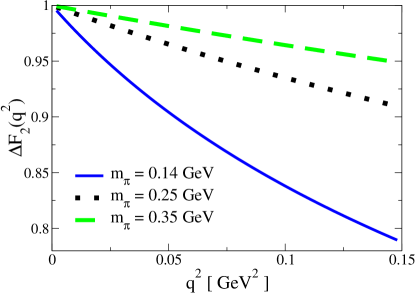
Figure 2: Plot of the isovector magnetic form factor’s deviation from linear $q^{2}$ behavior.

Using estimates of the low-energy constants: $g_{A}=1.25,|g_{{\Delta}N}|=1.5$, $M=0.94\,\texttt{GeV}$, $\Delta=0.29\,\texttt{GeV}$, and $\mu_{1}=3.38$; we plot the deviation from linearity of the one-loop result for the $F_{2}$ form factor in Fig. 2 for various values of the pion mass. This is done using the function ${\Delta}F_{2}(q^{2})$ defined by

$${\Delta}F_{2}(q^{2})=\frac{F_{2}(q^{2})-F_{2}(0)}{q^{2}F^{\prime}_{2}(0)}.$$ (24)

The plot shows considerable deviation from linearity at the physical pion mass. For lattice pion masses around $0.25$ to $0.35\,\texttt{GeV}$, there is a $\sim 5-10\%$ deviation from linear behavior. As the lattice pion masses are brought down at fixed lattice spacing (so that the minimal $q^{2}$ remains fixed), there is a clear trend toward non-linear behavior in $q^{2}$.

We must keep in mind that the results plotted in the Figure receive $\sim 30\%$ corrections for pion masses around $0.35\,\texttt{GeV}$ due to higher-order terms in the chiral expansion that scale as $m_{\pi}/\Lambda_{\chi}$ Meissner and Steininger (1997); Puglia and Ramsey-Musolf (2000). Such corrections are independent of $q^{2}$. Beyond $q^{2}\sim 0.1\,\texttt{GeV}\,{}^{2}$ there are $\sim 30\%$ corrections from recoil $q^{2}/M^{2}$ terms in loop graphs that contribute to the deviation from linearity Kubis and Meissner (2001). The Figure shows that non-linear $q^{2}$ behavior is to be expected from the magnetic form factor for moderate pion masses. The EFT, however, is at a loss to describe the lattice data at the minimal lattice momentum transfer available on current dynamical lattices: $q^{2}=0.25\,\texttt{GeV}\,{}^{2}$ lies far off the axis in the plot, certainly too far to utilize the EFT.

IV.2 Twisted Boundary Conditions and Finite Volume Modifications

From our discussion in Sect. III, we know that the restriction to discrete lattice momentum can be circumvented by using partially twisted boundary conditions and calculating matrix elements of the isospin raising operator, see Eq. (12). We demonstrate that this is the case by calculating the isovector magnetic form factor using partially twisted baryon $\chi$PT. Additionally by using this theory at finite volume, we can deduce the dynamical effects due to the boundary conditions. These effects are systematic errors that must be removed to determine the form factor.

IV.2.1 Partially Twisted and Partially Quenched $\chi$PT

In the meson sector of partially quenched $\chi$PT (PQ$\chi$PT) Bernard and Golterman (1994); Sharpe (1997); Golterman and Leung (1998); Sharpe and Shoresh (2000, 2001), the coset field $\Sigma$, which satisfies twisted boundary conditions, can be traded in for the field ${\tilde{\Sigma}}$ defined by ${\tilde{\Sigma}}(x)=V^{\dagger}(x){\Sigma}(x)V(x)$, which is periodic at the boundary Sachrajda and Villadoro (2005). In terms of this field, the Lagrangian of PQ$\chi$PT appears as

$${\mathcal{L}}=\frac{f^{2}}{8}\text{str}\left({\tilde{D}}_{\mu}{\tilde{\Sigma}}{\tilde{D}}_{\mu}{\tilde{\Sigma}}^{\dagger}\right)-{\lambda}\,\text{str}\left(m_{Q}^{\dagger}{\tilde{\Sigma}}+{\tilde{\Sigma}}^{\dagger}m_{Q}\right).$$ (25)

The action of the covariant derivative ${\tilde{D}}^{\mu}$ is specified in Eq. (17).

To include baryons into PQ$\chi$PT, one uses rank three flavor tensors Labrenz and Sharpe (1996). The spin-$\frac{1}{2}$ baryons are described by the $\bm{70}$-dimensional supermultiplet ${\mathcal{B}}^{ijk}$, while the spin-$\frac{3}{2}$ baryons are described by the $\bm{44}$-dimensional supermultiplet ${\mathcal{T}}_{\mu}^{ijk}$ Beane and Savage (2002). The baryon flavor tensors we use, however, are twisted at the boundary of the lattice. Thus we define new tensors ${\tilde{\mathcal{B}}}^{ijk}$ and ${\tilde{\mathcal{T}}}_{\mu}^{ijk}$ both having the form Tiburzi (2005a)

$${\tilde{\mathcal{B}}}_{ijk}(x)=V^{\dagger}_{ii}(x)V^{\dagger}_{jj}(x)V^{\dagger}_{kk}(x){\mathcal{B}}_{ijk}(x).$$ (26)

These baryon fields satisfy periodic boundary conditions and their free and leading-order interaction Lagrangian has been given in Tiburzi (2005a).

In partially quenched QCD, the isovector vector current is defined by $J_{\mu}^{a}(x)={\overline{Q}}(x)\,{\overline{T}}{}^{a}\gamma_{\mu}Q(x)$. The choice of supermatrices ${\overline{T}}{}^{a}$ is not unique Golterman and Pallante (2001), even when one imposes the condition $\text{str}\,{\overline{T}}{}^{a}=0$. One should choose a form of the supermatrices that maintains the cancellation of valence and ghost quark loops with an operator insertion Tiburzi (2005b); Detmold and Lin (2005). For the flavor changing contributions we consider below, however, these operator self-contractions automatically vanish. For our calculation we require the action of $J_{\mu}^{a}$ in only the valence sector, and specify the upper $2\times 2$ block of ${\overline{T}}{}^{a}$ to be the usual isospin generators $T^{a}$. Henceforth we restrict our attention to the operator $J_{\mu}^{+}\equiv J_{\mu}^{1}+iJ_{\mu}^{2}$.

In calculating the isovector magnetic moment of the nucleon at next-to-leading order in the chiral expansion, there are local operators that contribute at tree level. In $\chi$PT, the leading isovector current operator is

$${\delta}J_{\mu}^{+}=\frac{\mu_{1}}{M}\partial_{\nu}\left({\overline{N}}\sigma_{\mu\nu}T^{+}N\right).$$ (27)

In partially twisted PQ$\chi$PT, there are two terms in the leading isovector current operator

$${\delta}J_{\mu}^{+}=\frac{1}{M}{\tilde{D}}_{\nu}\left[\mu_{\alpha}\left({\overline{{\tilde{\mathcal{B}}}}}\,\sigma_{\mu\nu}{\tilde{\mathcal{B}}}\,{\overline{T}}{}^{+}\right)+\mu_{\beta}\left({\overline{{\tilde{\mathcal{B}}}}}\,\sigma_{\mu\nu}{\overline{T}}{}^{+}{\tilde{\mathcal{B}}}\right)\right].$$ (28)

The contribution of these operators at tree level is proportional to the linear combination $\frac{1}{3}\mu_{\alpha}-\frac{1}{6}\mu_{\beta}$, which is identical to the $\chi$PT low-energy constant $\mu_{1}$ as can be demonstrated by matching Beane and Savage (2002).

IV.2.2 Partially Twisted Isovector Magnetic Form Factor

In the infinite volume limit, the isovector magnetic moment can be extracted from the matrix element

$$\langle p(\bm{q})\downarrow|J_{3}^{+}|n(\bm{0})\uparrow\rangle=\frac{-iq}{2M}F_{2}(q^{2}),$$ (29)

in the case where $\bm{q}=(0,q,0)$. On the lattice, we can take both the source and sink to be at zero momentum, so that $\bm{q}=\bm{0}$. Momentum transfer can then be induced by giving the valence up and down quarks different twist angles. For simplicity we choose $\bm{B}^{d}=\bm{0}$ and $\bm{B}^{u}=(0,B,0)$. Calculation of the infinite volume isovector form factor then proceeds similarly to that above in Sect. IV.1. In partially twisted baryon $\chi$PT, there are additional diagrams that contribute involving the hairpin interaction. These diagrams are shown in Fig. 3. The sum of all hairpin diagrams, however, vanishes. With $m_{j}=m_{u}$, the infinite volume contributions from the diagrams in the Figure are identical to $F_{2}(q^{2})$ in Eq. (22) under the simple replacement $q\to B$. This is the kinematic effect we expect from raising isospin with a twisted $u$-quark.

Figure 3: One-loop contributions to the isospin transition matrix elements in partially twisted heavy baryon $\chi$PT. Nucleons (deltas) are represented by single (double) lines, while mesons are represented by dashed lines. The cross is the hairpin interaction, and the wiggly line shows the insertion of the isospin raising operator.

Dynamical effects due to twisted boundary conditions arise from the propagation of the light Goldstone modes to the boundary. The sensitivity of these modes to the boundary conditions must be taken into account and can be done so in a model-independent way using baryon $\chi$PT in finite volume. The modification to the effective theory is straightforward. In effect, we replace the integrals over loop momenta with sums over the allowed modes $\bm{k}=2\pi\bm{n}/L$. The twisting is already taken into account in the effective theory by the $U(1)$ gauge covariant derivative ${\tilde{D}}_{\mu}$ above. The Poisson re-summation formula then allows us to cast these sums into the infinite volume result plus the finite volume modification.

There are, however, further contributions from using the partially twisted chiral theory in a box. Diagrams that ordinarily vanish in infinite volume can now make contributions in a finite volume. This is the case for the diagrams depicted in Fig. 4. Quite interestingly these diagrams are only non-vanishing in a finite volume with twisted boundary conditions. When the twisting parameters vanish, so too does this finite volume effect. This can easily be explained. In infinite volume the diagrams in Fig. 4 vanish due to $SO(4)$ rotational invariance, while in a periodic finite volume they vanish due to invariance under lattice rotations. Lattice rotational invariance is broken in the direction of the twisted boundary conditions, hence the diagrams make non-vanishing contributions. Notice that the hairpin diagrams each vanish because the flavor-neutral mesons are additionally neutral under $B_{\mu}$.

Figure 4: Additional one-loop contributions to the isospin transition matrix elements. Diagram elements are the same as in Fig. 3. These diagrams vanish for periodic fields in a finite volume.

Combining the infinite volume and finite volume results with a twisted valence $u$-quark and specifying the case $m_{j}=m_{u}$, we arrive at

$$\langle p(\bm{0})\downarrow|J_{3}^{+}|n(\bm{0})\uparrow\rangle = \frac{-iB}{2M}\Bigg{(}F_{2}(B^{2})-\frac{g_{A}^{2}M}{4\pi^{2}f^{2}B}{\mathcal{K}}_{2}(m_{\pi},B\hat{y},0)-\frac{g_{{\Delta}N}^{2}M}{36\pi^{2}f^{2}B}{\mathcal{K}}_{2}(m_{\pi},B\hat{y},{\Delta})$$ (30)

$$+\frac{3M}{4\pi^{2}f^{2}}\int_{0}^{1}dx\,\Big{\{}g_{A}^{2}{\mathcal{L}}_{33}[m_{\pi}P_{\pi}(x,B^{2}),xB\hat{y},0]$$

$$\phantom{bigspacererer}+\frac{2}{9}g_{{\Delta}N}^{2}{\mathcal{L}}_{33}[m_{\pi}P_{\pi}(x,B^{2}),xB\hat{y},{\Delta}]\Big{\}}\Bigg{)},$$

where $F_{2}(B^{2})$ is given in Eq. (22). The effects of the finite volume are encoded in the functions ${\mathcal{K}}_{2}(m,\bm{B},{\Delta})$ and ${\mathcal{L}}_{33}(m,\bm{B},{\Delta})$, which are defined in the Appendix. In the limit that $B\to 0$, the result above accordingly vanishes: $B$ functions as a momentum transfer which is necessary for the magnetic form factor to be visible. Taking the derivative

$$\lim_{B\to 0}\frac{2Mi}{B}\langle p(\bm{0})\downarrow|J_{3}^{+}|n(\bm{0})\uparrow\rangle,$$

we can extract the magnetic moment $F_{2}(0)$ up to additive volume corrections. The corrections at $B=0$ involving the ${\mathcal{L}}_{33}(m_{\pi},\bm{0},{\Delta})$ function are identical to the finite volume results in Beane (2004). Those results, however, were derived under the assumption that a momentum extrapolation to zero had been performed, or alternately that one had employed a background magnetic field. Devoid of these assumptions, the current insertion method produces a second finite volume correction to the magnetic moment involving

$$\frac{\partial{\mathcal{K}}_{2}(m_{\pi},B\hat{y},{\Delta})}{\partial B}\Big{|}_{B=0}.$$

To investigate the effect of the finite volume on the extraction of the isovector magnetic moment using twisted boundary conditions, we define the relative difference

$${\delta}_{L}[F_{2}(B^{2})]=\frac{\frac{2Mi}{B}\langle p(\bm{0})\downarrow|J_{3}^{+}|n(\bm{0})\uparrow\rangle-F_{2}(B^{2})}{F_{2}(B^{2})}.$$ (31)

In the limit $B\to 0$, the difference is just ${\delta}_{L}[F_{2}(0)]={\delta}_{L}[\mu]$, the relative difference in the magnetic moment. In Fig. 5, we plot ${\delta}_{L}[\mu]$ as a function of $L$ for various values of the pion mass to contrast our results with those of Ref. Beane (2004).

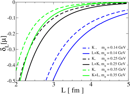
Figure 5: Comparison of finite volume effects for the isovector magnetic moment. Plotted versus $L$ is the relative difference ${\delta}_{L}[\mu]$ for a few values of the pion mass. The total finite volume effect is denoted by $K+L$, while the contribution to ${\delta}_{L}[\mu]$ from $\partial{\mathcal{K}}_{2}/\partial B$ alone is denoted by $K$.

We plot the total contribution to ${\delta}_{L}[\mu]$ which arises from both the $\partial{\mathcal{K}}_{2}/\partial B$, and ${\mathcal{L}}_{33}$ functions in Eq. (30), as well as just the contribution from $\partial{\mathcal{K}}_{2}/\partial B$. The latter is the dominant finite volume effect. Of course, to extract the magnetic moment, we require ${\theta}\neq 0$ and thus we investigate ${\delta}_{L}[F_{2}(B^{2})]$ in Eq. (31). In Fig. 6, we fix the lattice volume at $2.5\,\texttt{fm}$ and plot the relative difference ${\delta}_{L}[F_{2}(B^{2})]$ as a function of ${\theta}$ for a few values of the pion mass. We see that the effect of the finite volume decreases with ${\theta}$. Generally the volume effects with momentum transfer (here the momentum transfer $q=B={\theta}/L$) are smaller than those at zero momentum transfer. In Detmold and Lin (2005) this was anticipated due to the loop pion mass appearing as $m_{\pi}^{2}+x(1-x)q^{2}>m_{\pi}^{2}$. There is also a simple physical interpretation for this effect: with a space-like momentum transfer the correlation function is being probed on distances of order $\sim 1/\sqrt{q^{2}}$. As $q^{2}$ increases, the resolving power of the virtual probe diminishes the volume effect.

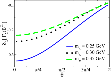
Figure 6: Finite volume effects for extracting the isovector magnetic moment. Plotted versus ${\theta}$ is the relative difference ${\delta}_{L}[F_{2}(B^{2})]$ for a few values of the pion mass. The momentum transfer from twisting is $B={\theta}\times 0.079\,\texttt{GeV}$

While twisted boundary conditions have introduced systematic error into the determination of the isovector moment, we stress that this is a controlled error. In a fixed box size, we need only know the low-energy constants $g_{A}$, $g_{{\Delta}N}$, ${\Delta}$, and $f_{\pi}$ to remove this effect. Without twisting, one must rely on phenomenological or other fitting functions which introduce uncontrolled error. With twisting, however, the lattice practitioner can approach the calculation of the isovector magnetic moment from various ways in conjunction with the EFT. For example, one can choose values of ${\theta}\sim 0.1$ to eliminate the need for a momentum extrapolation, cf Fig. 2. One must then use the EFT to remove the $\sim 25\%$ volume effects. Alternately one could choose ${\theta}\lesssim\pi$ to minimize the effect of the finite volume. For these values of ${\theta}$ one then uses the momentum dependence predicted by the EFT, cf Eq. (22), to obtain the magnetic moment. Another virtue to the EFT approach is that higher-order corrections to the quark mass, volume, and momentum-transfer dependence can be calculated to aid in the extrapolation. Although we have focused on the magnetic moment, the expressions we have derived here are also relevant for the isovector magnetic radius.

As a final point, an assumption inherent in our discussion is that no multi-particle thresholds are reached. For large enough momenta, multi-particle thresholds are inevitably reached. Volume corrections are no longer exponentially suppressed in asymptotic volumes; they become power law and will likely dwarf any signal. For the extraction of moments and radii of stable particles near zero momentum transfer, however, we are safely away from the multi-particle continuum.

V Summary

We have related matrix elements of arbitrary quark bilinear operators that change isospin to isovector combinations of those that do not change isospin. Using flavor twisted boundary conditions on the valence quark fields, form factors of these isovector matrix elements can then be deduced from the lattice at continuous values of the momentum transfer. Isovector moments and radii can thus be determined from simulations at zero lattice momentum. Using twisted boundary conditions on the quark fields dramatically modifies the effect of the finite volume, even away from multi-particle cuts. This systematic effect can be handled with EFTs. The determination of isovector moments and radii without any model-dependent assumptions about the momentum dependence is thus well within reach of current resources.

Finite Volume Functions

In this Appendix, we define and evaluate the finite volume functions contributing to the isovector magnetic form factor. These functions can be related to a more basic sum that is ubiquitously encountered in these calculations

$${\mathcal{I}}_{\alpha}(\bm{B},{\beta}^{2})=\frac{1}{L^{3}}\sum_{\bm{k}}\frac{1}{[(\bm{k}+\bm{B})^{2}+{\beta}^{2}]^{\alpha}}-\int\frac{d\bm{k}}{(2\pi)^{3}}\frac{1}{[(\bm{k}+\bm{B})^{2}+{\beta}^{2}]^{\alpha}},$$ (32)

which can be cast into an exponentially convergent form involving elliptic theta functions Sachrajda and Villadoro (2005). In the text, the function ${\mathcal{K}}_{2}(m,\bm{B},{\Delta})$ is defined by

$${\mathcal{K}}_{2}(m,\bm{B},{\Delta}) = \frac{8\pi^{2}}{L^{3}}\int_{0}^{\infty}d{\lambda}\sum_{\bm{k}}\frac{k_{2}+B_{2}}{[(\bm{k}+\bm{B})^{2}+{\beta}_{\Delta}^{2}]^{3/2}},$$ (33)

with ${\beta}_{\Delta}^{2}={\lambda}^{2}+2{\Delta}{\lambda}+m^{2}$. Using the expression for ${\mathcal{I}}_{1/2}$ in terms of elliptic theta functions, the integral over ${\lambda}$ can then be expressed in terms of the $\operatorname{Erfc}(x)$ function Arndt and Lin (2004). The final result appears as the one-dimensional integral

$${\mathcal{K}}_{2}(m,B\hat{y},{\Delta})=-\frac{\sqrt{\pi}L}{4}\int_{0}^{\infty}d\tau\,\tau^{-5/2}e^{\tau({\Delta}^{2}-m^{2})}\operatorname{Erfc}({\Delta}\sqrt{\tau})\vartheta^{\prime}_{3}\left(\frac{BL}{2},e^{-\frac{L^{2}}{4\tau}}\right)\vartheta_{3}\left(0,e^{-\frac{L^{2}}{4\tau}}\right)^{2},$$ (34)

with $\vartheta_{3}(q,z)$ as the Jacobi elliptic theta function of the third kind. Lastly the function ${\mathcal{L}}_{33}(m,\bm{B},{\Delta})$ is given by

$${\mathcal{L}}_{33}(m,B\hat{y},{\Delta}) = 8\pi^{2}\int_{0}^{\infty}d{\lambda}\left[\frac{1}{L^{3}}\sum_{\bm{k}}\frac{(k_{3})^{2}}{[(\bm{k}+\bm{B})^{2}+{\beta}_{\Delta}^{2}]^{5/2}}-\int\frac{d\bm{k}}{(2\pi)^{3}}\frac{(k_{3})^{2}}{[(\bm{k}+\bm{B})^{2}+{\beta}_{\Delta}^{2}]^{5/2}}\right]$$ (35)

$$= \frac{\sqrt{\pi}}{3}\int_{0}^{\infty}d\tau\,\tau^{-3/2}e^{\tau({\Delta}^{2}-m^{2})}\operatorname{Erfc}({\Delta}\sqrt{\tau})\Bigg{[}\vartheta_{3}\left(0,e^{-\frac{L^{2}}{4\tau}}\right)^{2}\vartheta_{3}\left(\frac{BL}{2},e^{-\frac{L^{2}}{4\tau}}\right)$$

$$\phantom{spacererer}+\frac{L^{2}}{8\tau}\vartheta^{\prime\prime}_{3}\left(0,e^{-\frac{L^{2}}{4\tau}}\right)\vartheta_{3}\left(0,e^{-\frac{L^{2}}{4\tau}}\right)\vartheta_{3}\left(\frac{BL}{2},e^{-\frac{L^{2}}{4\tau}}\right)-1\Bigg{]}.$$

References

- Bernard et al. (2003) C. Bernard et al., Nucl. Phys. Proc. Suppl. 119, 170 (2003), eprint hep-lat/0209086.
- Wilcox (2002) W. Wilcox, Phys. Rev. D66, 017502 (2002), eprint hep-lat/0204024.
- Gross and Kitazawa (1982) D. J. Gross and Y. Kitazawa, Nucl. Phys. B206, 440 (1982).
- Roberge and Weiss (1986) A. Roberge and N. Weiss, Nucl. Phys. B275, 734 (1986).
- Wiese (1992) U. J. Wiese, Nucl. Phys. B375, 45 (1992).
- Luscher et al. (1996) M. Luscher, S. Sint, R. Sommer, and P. Weisz, Nucl. Phys. B478, 365 (1996), eprint hep-lat/9605038.
- Bucarelli et al. (1999) A. Bucarelli, F. Palombi, R. Petronzio, and A. Shindler, Nucl. Phys. B552, 379 (1999), eprint hep-lat/9808005.
- Guagnelli et al. (2003) M. Guagnelli et al. (Zeuthen-Rome / ZeRo), Nucl. Phys. B664, 276 (2003), eprint hep-lat/0303012.
- Kiskis et al. (2002) J. Kiskis, R. Narayanan, and H. Neuberger, Phys. Rev. D66, 025019 (2002), eprint hep-lat/0203005.
- Kiskis et al. (2003) J. Kiskis, R. Narayanan, and H. Neuberger, Phys. Lett. B574, 65 (2003), eprint hep-lat/0308033.
- Kim and Christ (2003) C.-H. Kim and N. H. Christ, Nucl. Phys. Proc. Suppl. 119, 365 (2003), eprint hep-lat/0210003.
- Kim (2004) C.-H. Kim, Nucl. Phys. Proc. Suppl. 129, 197 (2004), eprint hep-lat/0311003.
- Bedaque (2004) P. F. Bedaque, Phys. Lett. B593, 82 (2004), eprint nucl-th/0402051.
- de Divitiis et al. (2004) G. M. de Divitiis, R. Petronzio, and N. Tantalo, Phys. Lett. B595, 408 (2004), eprint hep-lat/0405002.
- Sachrajda and Villadoro (2005) C. T. Sachrajda and G. Villadoro, Phys. Lett. B609, 73 (2005), eprint hep-lat/0411033.
- Bedaque and Chen (2005) P. F. Bedaque and J.-W. Chen, Phys. Lett. B616, 208 (2005), eprint hep-lat/0412023.
- Tiburzi (2005a) B. C. Tiburzi, Phys. Lett. B617, 40 (2005a), eprint hep-lat/0504002.
- Flynn et al. (2006) J. M. Flynn, A. Juttner, and C. T. Sachrajda (UKQCD), Phys. Lett. B632, 313 (2006), eprint hep-lat/0506016.
- Guadagnoli et al. (2006) D. Guadagnoli, F. Mescia, and S. Simula, Phys. Rev. D73, 114504 (2006), eprint hep-lat/0512020.
- Aarts et al. (2006) G. Aarts, C. Allton, J. Foley, S. Hands, and S. Kim (2006), eprint hep-lat/0607012.
- Jenkins and Manohar (1991a) E. Jenkins and A. V. Manohar, Phys. Lett. B255, 558 (1991a).
- Jenkins and Manohar (1991b) E. Jenkins and A. V. Manohar, Phys. Lett. B259, 353 (1991b).
- Bernard et al. (1992) V. Bernard, N. Kaiser, J. Kambor, and U. G. Meissner, Nucl. Phys. B388, 315 (1992).
- Bernard et al. (1995) V. Bernard, N. Kaiser, and U.-G. Meissner, Int. J. Mod. Phys. E4, 193 (1995), eprint hep-ph/9501384.
- Jenkins et al. (1993) E. Jenkins, M. E. Luke, A. V. Manohar, and M. J. Savage, Phys. Lett. B302, 482 (1993), eprint hep-ph/9212226.
- Bernard et al. (1998) V. Bernard, H. W. Fearing, T. R. Hemmert, and U. G. Meissner, Nucl. Phys. A635, 121 (1998), eprint hep-ph/9801297.
- Meissner and Steininger (1997) U.-G. Meissner and S. Steininger, Nucl. Phys. B499, 349 (1997), eprint hep-ph/9701260.
- Puglia and Ramsey-Musolf (2000) S. J. Puglia and M. J. Ramsey-Musolf, Phys. Rev. D62, 034010 (2000), eprint hep-ph/9911542.
- Kubis and Meissner (2001) B. Kubis and U. G. Meissner, Eur. Phys. J. C18, 747 (2001), eprint hep-ph/0010283.
- Bernard and Golterman (1994) C. W. Bernard and M. F. L. Golterman, Phys. Rev. D49, 486 (1994), eprint [http://arXiv.org/abs]hep-lat/9306005.
- Sharpe (1997) S. R. Sharpe, Phys. Rev. D56, 7052 (1997), eprint [http://arXiv.org/abs]hep-lat/9707018.
- Golterman and Leung (1998) M. F. L. Golterman and K.-C. Leung, Phys. Rev. D57, 5703 (1998), eprint [http://arXiv.org/abs]hep-lat/9711033.
- Sharpe and Shoresh (2000) S. R. Sharpe and N. Shoresh, Phys. Rev. D62, 094503 (2000), eprint [http://arXiv.org/abs]hep-lat/0006017.
- Sharpe and Shoresh (2001) S. R. Sharpe and N. Shoresh, Phys. Rev. D64, 114510 (2001), eprint [http://arXiv.org/abs]hep-lat/0108003.
- Labrenz and Sharpe (1996) J. N. Labrenz and S. R. Sharpe, Phys. Rev. D54, 4595 (1996), eprint [http://arXiv.org/abs]hep-lat/9605034.
- Beane and Savage (2002) S. R. Beane and M. J. Savage, Nucl. Phys. A709, 319 (2002), eprint hep-lat/0203003.
- Golterman and Pallante (2001) M. Golterman and E. Pallante, JHEP 10, 037 (2001), eprint hep-lat/0108010.
- Tiburzi (2005b) B. C. Tiburzi, Phys. Rev. D71, 054504 (2005b), eprint hep-lat/0412025.
- Detmold and Lin (2005) W. Detmold and C. J. D. Lin, Phys. Rev. D71, 054510 (2005), eprint hep-lat/0501007.
- Beane (2004) S. R. Beane, Phys. Rev. D70, 034507 (2004), eprint hep-lat/0403015.
- Arndt and Lin (2004) D. Arndt and C. J. D. Lin, Phys. Rev. D70, 014503 (2004), eprint hep-lat/0403012.