Abstract

We study the contributions $\Sigma_{0}$ and $\Sigma_{1}$, proportional to $a^{0}$ and $a^{1}$, to the fermion self-energy in Wilson’s formulation of lattice QCD with UV-filtering in the fermion action. We derive results for $m_{\mathrm{crit}}$ and the renormalization factors $Z_{S},Z_{P},Z_{V},Z_{A}$ to 1-loop order in perturbation theory for several filtering recipes (APE, HYP, EXP, HEX), both with and without a clover term. The perturbative series is much better behaved with filtering, in particular tadpole resummation proves irrelevant. Our non-perturbative data for $m_{\mathrm{crit}}$ and $Z_{A}/(Z_{m}Z_{P})$ show that the combination of filtering and clover improvement efficiently reduces the amount of chiral symmetry breaking – we find residual masses $am_{\mathrm{res}}=O(10^{-2})$.

1 Introduction

The Wilson formulation of lattice QCD breaks the chiral symmetry among the light flavors [1, 2]. Accordingly, Wilson fermions undergo an additive (and multiplicative) mass renormalization. While this is not a problem in principle – the explicit breaking disappears if the lattice spacing $a$ is sent to zero [3] – it entails a number of complications in numerical work based on this formulation. There are several strategies how the additive mass renormalization might be reduced. A popular choice, to augment the action by a clover term, has the merit of reducing cut-off effects from $O(a)$ to $O(ag_{0}^{2},...,a^{2})$ [4, 5, 6]. Another possibility, referred to as UV-filtering, is to replace all covariant derivatives in the fermion action by smeared descendents, as proposed in a staggered context [7, 8, 9] and later applied to Wilson/clover fermions [10, 11, 12, 13, 14]. We find that filtering indeed ameliorates important technical properties of the Wilson operator, as does the clover term without filtering. The real improvement, however, comes from combining the two.

With standard conventions the ($r\!=\!1$) Wilson operator takes the form

$$D_{\mathrm{W}}(x,y)={1\over 2}\sum_{\mu}\Big{\{}(\gamma_{\mu}-I)U_{\mu}(x)\delta_{x+\hat{\mu},y}-(\gamma_{\mu}+I)U_{\mu}^{\dagger}(x-\hat{\mu})\delta_{x-\hat{\mu},y}\Big{\}}+{1\over 2\kappa}\delta_{x,y}$$ (1)

where $I$ is the identity in spinor space. The Sheikholeslami-Wohlert “clover” operator follows by adding a hermitean contribution proportional to the gauge field strength [5]

$$D_{\mathrm{SW}}(x,y)=D_{\mathrm{W}}(x,y)-{c_{\mathrm{SW}}\over 2}\sum_{\mu<\nu}\sigma_{\mu\nu}F_{\mu\nu}\;\delta_{x,y}$$ (2)

with $\sigma_{\mu\nu}\!=\!{\mathrm{i}\over 2}[\gamma_{\mu},\gamma_{\nu}]$ and $F_{\mu\nu}$ the hermitean “clover-leaf” operator. In order to cancel the $O(a)$ contributions, the coefficient $c_{\mathrm{SW}}$ needs to be properly tuned. In perturbation theory one finds $c_{\mathrm{SW}}\!=\!1$ at the tree-level and a correction proportional to the $n$-th power of $g_{0}^{2}$ at the $n$-loop level. It is well known that for the standard “thin link” operator perturbation theory shows rather bad convergence properties. Therefore, the ALPHA collaboration has started a non-perturbative improvement program [15]. Another approach is to resum the tadpole contributions [16], since they are quite sizable. For filtered Wilson/clover quarks this might be different – we elaborate on “fat link” perturbation theory [11, 17, 18, 14], and we compare these predictions to (non-perturbative) data. It turns out that filtered perturbation theory shows a much better convergence behavior, but still, it does not describe the data very accurately. The agreement is (at accessible couplings) much better than in the unfiltered theory, but it is far from being completely satisfactory. We find that the additive mass shift is two orders of magnitude smaller than without filtering, and this is extremely useful in phenomenological studies.

The following two sections contain our perturbative results for UV-filtered Wilson/clover fermions. Sect. 2 focuses on the additive mass shift with $1,2,3$ steps of APE, HYP, EXP, HEX filtering and arbitrary improvement coefficient $c_{\mathrm{SW}}$. Sect. 3 contains our 1-loop results for the renormalization factors $Z_{S},Z_{P},Z_{V},Z_{A}$ with these filterings, a reminder how improved currents are constructed, and a comment on tadpole resummation. Sect. 4 presents our non-perturbative data for the additive mass shift and some renormalization factors, both with $c_{\mathrm{SW}}\!=\!0$ and $c_{\mathrm{SW}}\!=\!1$. Sect. 5 contains our summary. Details of “fat-link” perturbation theory, of an explicit mass shift calculation and of the parameter dependence have been arranged in three appendices.

2 Additive mass shift with UV filtering in 1-loop PT

In this paper we consider four types of filtering: APE, HYP, EXP, HEX. The fist two are well known [19, 9], the third one has been named “stout” in [20], and the fourth one is a straightforward application of the hypercubic nesting trick on the latter (see App. A for details). While on a technical level the smearing produces a smoothed gauge background, it is in fact a different choice of the discretization of the covariant derivative in the Dirac operator and therefore leads to an irrelevant change of the fermionic action (provided the filtering recipe is unchanged when taking the continuum limit).

In our analytical and numerical investigations we use the “standard” parameters

$$\alpha_{\mathrm{std}}^{\mathrm{APE}}\!=\!0.6\;,\qquad\alpha_{\mathrm{std}}^{\mathrm{EXP}}\!=\!0.1$$ (3)

for APE and EXP smearing, and similarly the “standard” parameters

$$\alpha_{\mathrm{std}}^{\mathrm{HYP}}\!=\!(0.75,0.6,0.3)\;,\qquad\alpha_{\mathrm{std}}^{\mathrm{HEX}}\!=\!(0.125,0.15,0.15)$$ (4)

for HYP and HEX smearing. The two values in (3) are related by giving an identical 1-loop prediction for all quantities of interest (e.g. $-am_{\mathrm{crit}}$), and the same statement holds for the hypercubically nested recipes (4), see App. A for details. Accordingly, all perturbative tables with label “APE” will apply to EXP, too, and ditto for a label “HYP” and the HEX recipe.

	thin link	1 APE	2 APE	3 APE	1 HYP
$c_{\mathrm{SW}}\!=\!0$	51.43471	13.55850	7.18428	4.81189	6.97653
$c_{\mathrm{SW}}\!=\!1$	31.98644	4.90876	1.66435	0.77096	1.98381
$c_{\mathrm{SW}}\!=\!2$	1.10790	-7.11767	-5.48627	-4.23049	-4.41059

Table 1: Additive mass shift $S$ for “thin link” Wilson or clover fermions and after APE or HYP filtering with standard parameters. The uncertainty is of order one in the last digit quoted.

The additive mass shift is given by the self-energy $\Sigma_{0}$ via [note that $am_{\mathrm{crit}}\!<\!0$ with (13)]

$$am_{\mathrm{crit}}=\Sigma_{0}=-{g_{0}^{2}\over 16\pi^{2}}C_{F}S+O(g_{0}^{4})$$ (5)

where $S$ is the quantity that is usually tabulated and $C_{F}\!=\!4/3$ for $SU(3)$ gauge group. Generalizing a standard calculation [21] to “fat-link” perturbation theory (see App. A for a summary) one may work out 1-loop predictions for $S$ [11, 18]. We have done this for arbitrary $c_{\mathrm{SW}}$. From inspecting Tab. 1 one notices that $c_{\mathrm{SW}}\!=\!1$ alone reduces the additive mass shift by a factor $1.6$. Filtering alone achieves a factor $3.8$ or $7.4$ with a single APE or HYP step, respectively. However, the combination reduces it by a factor $10.5$ or $26.0$, and hence proves much more efficient than any one of the ingredients alone. The tuned $c_{\mathrm{SW}}$ that would achieve zero mass shift is slightly above $2$ in the thin-link case, and slightly above $1$ in all cases with filtering. This is the first indication that filtered $c_{\mathrm{SW}}\!=\!1$ clover fermions break the chiral symmetry in a much milder way than filtered Wilson or unfiltered clover fermions. An important question is, of course, to which extent this is realized non-perturbatively, and we shall address this issue in due course.

3 Renormalization factors with UV filtering in 1-loop PT

3.1 Generic setup

In general, the matrix elements of some operator $O_{j}^{\mathrm{cont}}(\mu)$ in the continuum $\overline{\mathrm{MS}}$ scheme and its lattice counterparts $O_{k}^{\mathrm{latt}}(a)$ are related by

$$\langle.|O_{j}^{\mathrm{cont}}(\mu)|.\rangle=\sum_{k}Z_{jk}(a\mu)\langle.|O_{k}^{\mathrm{latt}}(a)|.\rangle$$ (6)

$$Z_{jk}(a\mu)=\delta_{jk}-{g_{0}^{2}\over 16\pi^{2}}(\Delta_{jk}^{\mathrm{latt}}-\Delta_{jk}^{\mathrm{cont}})=\delta_{jk}-{g_{0}^{2}\over 16\pi^{2}}C_{F}z_{jk}$$ (7)

with $C_{F}=4/3$ for $SU(3)$ gauge group. Typically (e.g. for 4-fermion operators and a non-chiral action), $k$ runs over other chiralities than $j$. For 2-fermion operators, this mixing shows up at higher orders in an expansion in the lattice spacing $a$, and packing it into the construction of improved currents, one is left with the diagonal term in (7). With our convention (which agrees with [21], but not with [14]) a value $z_{X}\!>\!0$ signals $Z_{X}\!<\!1$. Specifically (with $X\!=\!S,P,V,A$),

$$Z_{S}(a\mu)=1-{g_{0}^{2}\over 4\pi^{2}}\Big{[}{z_{S}\over 3}-\log(a^{2}\mu^{2})\Big{]}\;, Z_{V}=1-{g_{0}^{2}\over 12\pi^{2}}z_{V}$$ (8)

$$Z_{P}(a\mu)=1-{g_{0}^{2}\over 4\pi^{2}}\Big{[}{z_{P}\over 3}-\log(a^{2}\mu^{2})\Big{]}\;, Z_{A}=1-{g_{0}^{2}\over 12\pi^{2}}z_{A}$$ (9)

for the (pseudo-)scalar densities and the (axial-)vector currents, with corrections of order $O(g_{0}^{4})$ throughout.

3.2 Results for $Z_{S},Z_{P},Z_{V},Z_{A}$ for Wilson and clover fermions

The same approach of combining FORM-based [22] standard perturbative procedures [21] with “fat-link” perturbation theory that has been used in the previous section for the additive mass shift, allows one to work out the renormalization factors $Z_{S},Z_{P},Z_{V},Z_{A}$ for arbitrary $c_{\mathrm{SW}}$.

$c_{\mathrm{SW}}\!=\!0$	thin link	1 APE	2 APE	3 APE	1 HYP
$z_{S}$	12.95241	1.12593	-1.53149	-2.87223	-1.78317
$z_{P}$	22.59544	5.28288	1.07019	-0.98025	0.51727
$z_{V}$	20.61780	6.39810	3.62281	2.51381	3.38076
$z_{A}$	15.79628	4.31963	2.32197	1.56782	2.23054
$(z_{P}\!-\!z_{S})/2$	4.82152	2.07848	1.30084	0.94599	1.15022
$z_{V}\!-\!z_{A}$	4.82152	2.07847	1.30084	0.94599	1.15022

Table 2: Coefficient $z_{X}$ in formula (7) for the renormalization factor $Z_{X}$ with $X=S,P,V,A$ for $c_{\mathrm{SW}}\!=\!0$ Wilson fermions with APE or HYP filtering with standard parameters.

$c_{\mathrm{SW}}\!=\!1$	thin link	1 APE	2 APE	3 APE	1 HYP
$z_{S}$	19.30995	4.11106	0.40606	-1.43930	-0.03678
$z_{P}$	22.38259	4.80364	0.65185	-1.33218	0.12845
$z_{V}$	15.32907	3.31243	1.43934	0.82550	1.38517
$z_{A}$	13.79274	2.96614	1.31645	0.77195	1.30255
$(z_{P}\!-\!z_{S})/2$	1.53632	0.34629	0.12290	0.05356	0.08262
$z_{V}\!-\!z_{A}$	1.53633	0.34629	0.12289	0.05355	0.08262

1 HYP [14]
0.12
-0.04
1.38
1.30
-0.08
0.08

Table 3: Like Tab. 4, but for $c_{\mathrm{SW}}\!=\!1$ clover fermions. The last column has been adapted to our sign convention [cf. (7)] and suggests that there is a mislabeling in Tab. III of Ref. [14].

$c_{\mathrm{SW}}\!=\!2$	thin link	1 APE	2 APE	3 APE	1 HYP
$z_{S}$	22.90672	4.35133	0.06571	-1.91937	-0.43671
$z_{P}$	26.24177	6.10928	1.39146	-0.81914	0.80287
$z_{V}$	8.95400	-0.33664	-1.07948	-1.08366	-0.89073
$z_{A}$	7.28648	-1.21561	-1.74236	-1.63378	-1.51052
$(z_{P}\!-\!z_{S})/2$	1.66753	0.87898	0.66288	0.55012	0.61979
$z_{V}\!-\!z_{A}$	1.66752	0.87897	0.66288	0.55012	0.61979

Table 4: Like Tab. 4, but for $c_{\mathrm{SW}}\!=\!2$. This nails down the full polynomial dependence on $c_{\mathrm{SW}}$.

Our results for $z_{X}$ with $X\!=\!S,P,V,A$ in the unimproved case $c_{\mathrm{SW}}\!=\!0$ are summarized in Tab. 4. An important check is that $(z_{P}\!-\!z_{S})/2$ and $z_{V}\!-\!z_{A}$ should coincide [23]. The pertinent entries indicate that the integration routine yields at least 6 significant digits.

Our results for $z_{X}$ with $X\!=\!S,P,V,A$ in the improved case $c_{\mathrm{SW}}\!=\!1$ are summarized in Tab. 4. Again we check the quality of the agreement between $(z_{P}\!-\!z_{S})/2$ and $z_{V}\!-\!z_{A}$. Moreover, since these figures indicate the amount of chiral symmetry breaking [23], it is instructive to compare the bottom lines of Tab. 4 to those of Tab. 4. Improvement alone reduces $z_{V}\!-\!z_{A}$ by a factor $3.1$. One step of APE or HYP filtering diminishes it by a factor $2.3$ or $4.2$, respectively. However, the combination of these recipes achieves a factor $13.9$ or $58.4$, and hence proves much more efficient that any of the ingredients alone. This is in line with the lesson learned from Tab. 1.

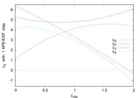
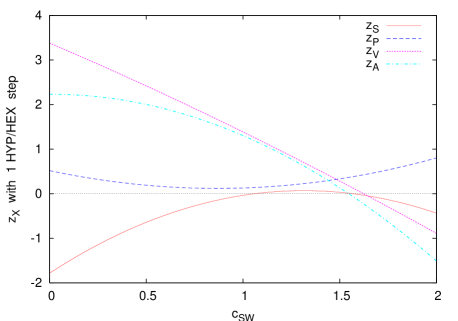
Figure 1: Finite pieces $z_{S,P,V,A}$ of the $Z_{X}$ for 1 APE and 1 HYP fermions as a function of $c_{\mathrm{SW}}$.

Our results for $z_{X}$ in the case $c_{\mathrm{SW}}\!=\!2$ are shown in Tab. 4. Obviously, “too much” improvement deteriorates the chiral properties of the action. At 1-loop order all $z_{X}$ depend on $c_{\mathrm{SW}}$ through a quadratic polynomial, hence Tabs. 4 - 4 give them for arbitrary values of the Sheikholeslami-Wohlert parameter. For instance, for 1 HYP (or 1 HEX) step they imply

$$z_{S} = -1.78317+2.81955c_{\mathrm{SW}}-1.07316c_{\mathrm{SW}}^{2}$$

$$z_{P} = +0.51727-0.92044c_{\mathrm{SW}}+0.53162c_{\mathrm{SW}}^{2}$$

$$z_{V} = +3.38076-1.85544c_{\mathrm{SW}}-0.14015c_{\mathrm{SW}}^{2}$$

$$z_{A} = +2.23054+0.01455c_{\mathrm{SW}}-0.94254c_{\mathrm{SW}}^{2}$$ (10)

and from the pertinent curves (see Fig. 1) one learns two lessons. First, the point where the 1 HYP action is most chiral (i.e. where $z_{P}\!-\!z_{S}$ and $z_{V}\!-\!z_{A}$ are minimal) is near $c_{\mathrm{SW}}=1.1653$. Second, near $c_{\mathrm{SW}}\!=\!1.5$ the four coefficients $z_{S,P,V,A}$ are simultaneously small. By contrast, with less filtering (e.g. 1 APE) the point of minimal chiral symmetry breaking is further away from 1, and the four renormalization factors cannot be simultaneously close to 1.

Any strategy in which $c_{\mathrm{SW}}$ deviates, for large $\beta$, from $1$ by a polynomial in $g_{0}^{2}$ with vanishing constant part yields a theory with $O(ag_{0}^{2})$ cut-off effects. Here we restrict ourselves to $c_{\mathrm{SW}}\!=\!1$. Getting higher terms in the polynomial right reduces discretization effects to $O(ag_{0}^{4})$ or better, and non-perturbative improvement would realize $O(a^{2})$.

3.3 Construction of improved currents and densities

At tree-level $Z_{S,P,V,A}\!=\!1$, and the improvement coefficients are $c_{\mathrm{SW}}\!=\!1$, $b_{S,P,V,A}\!=\!1$, $b_{m}\!=\!-1/2$ and $c_{V,A}\!=\!0$. Accordingly, in a tree-level $O(a)$ improved theory the currents read

$$(S_{\mathrm{imp}})^{a} = (1+am_{q})S^{a}$$

$$(P_{\mathrm{imp}})^{a} = (1+am_{q})P^{a}$$

$$(V_{\mathrm{imp}})_{\mu}^{a} = (1+am_{q})V_{\mu}^{a}$$

$$(A_{\mathrm{imp}})_{\mu}^{a} = (1+am_{q})A_{\mu}^{a}$$ (11)

which is free of mixing effects, but it is well known that (at least in the unfiltered case) this is not sufficient to be in the Symanzik $O(a^{2})$ scaling regime for accessible couplings. Throughout, we use the flavor decomposition $X\!=\!X^{a}{\lambda^{a}\over 2}$ with $\lambda^{a}$ one of the Gell-Mann matrices ($a\!=\!1..8$).

At the 1-loop level and with ${N_{\!f}}\!=\!0,{N_{\!c}}\!=\!3$, renormalization factors in the unfiltered theory take the form $Z_{S}\!=\!1\!-\!0.163042g_{0}^{2}$, $Z_{P}\!=\!1\!-\!0.188986g_{0}^{2}$, $Z_{V}\!=\!1\!-\!0.129430g_{0}^{2}$, $Z_{A}\!=\!1\!-\!0.116458g_{0}^{2}$, as follows from the first column of Tab. 4. Similarly $c_{\mathrm{SW}}\!=\!1+0.2659g_{0}^{2}$ [5, 24], and $b_{S}\!=1\!+\!0.1925g_{0}^{2}$, $b_{P}\!=1\!+\!0.1531g_{0}^{2}$, $b_{V}\!=1\!+\!0.1532g_{0}^{2}$, $b_{A}\!=1\!+\!0.1522g_{0}^{2}$, $b_{m}\!=\!-1/2\!-\!0.09623g_{0}^{2}$, $c_{V}\!=\!-0.01633g_{0}^{2}$, $c_{A}\!=\!-0.00757g_{0}^{2}$, see [15, 25, 26, 27] for details. The main message is that most of the 1-loop corrections are large, since $g_{0}^{2}\!\simeq\!1$. With these expressions at hand, improved currents follow via

$$(S_{\mathrm{imp}})^{a} = Z_{S}\,\tilde{S}^{a}\,\quad,\qquad\,\tilde{S}^{a}=(1+b_{S}\,am_{q})\,S^{a}$$

$$(P_{\mathrm{imp}})^{a} = Z_{P}\,\tilde{P}^{a}\quad,\qquad\tilde{P}^{a}=(1+b_{P}\,am_{q})\,P^{a}$$

$$(V_{\mathrm{imp}})_{\mu}^{a} = Z_{V}\,\tilde{V}_{\mu}^{a}\quad,\qquad\tilde{V}_{\mu}^{a}=(1+b_{V}\,am_{q})\,[V_{\mu}^{a}+ac_{V}\bar{\partial}_{\nu}T_{\mu\nu}^{a}]$$

$$(A_{\mathrm{imp}})_{\mu}^{a} = Z_{A}\,\tilde{A}_{\mu}^{a}\quad,\qquad\tilde{A}_{\mu}^{a}=(1+b_{A}\,am_{q})\,[A_{\mu}^{a}+ac_{A}\bar{\partial}_{\mu}P^{a}]$$ (12)

where $\bar{\partial}_{\mu}\!=\!{1\over 2}(\partial_{\mu}\!+\!\partial_{\mu}^{*})$ denotes the forward-backward symmetric derivative. Clearly, this is a complicated mixing pattern involving even the tensor current. Still, with perturbative coefficients it remains (in the unfiltered theory) a challenge to reach those couplings where the Symanzik scaling with $O(a^{2})$ cut-off effects sets in. This is why (in the thin-link theory) a non-perturbative determination of the renormalization constants and improvement coefficients is preferred [15].

Our hope is that with filtering perturbative improvement at the 1-loop level is a viable strategy. An important check is how well the renormalized VWI quark mass and the renormalized AWI quark mass coincide. The (bare) Wilson or clover quark mass is defined as

$$m^{\mathrm{W}}=m_{0}-m_{\mathrm{crit}}\qquad\mbox{where}\qquad am_{0}={1\over 2}\Big{(}{1\over\kappa}-{1\over\kappa_{\mathrm{tree}}}\Big{)}\;,\quad am_{\mathrm{crit}}={1\over 2}\Big{(}{1\over\kappa_{\mathrm{crit}}}-{1\over\kappa_{\mathrm{tree}}}\Big{)}$$ (13)

with $\kappa_{\mathrm{tree}}\!=\!1/8$, and the (renormalized) VWI quark mass then follows through

$$m^{\mathrm{VWI}}(\mu)=Z_{m}(a\mu)(1+b_{m}am^{\mathrm{W}})m^{\mathrm{W}}\;.$$ (14)

The (bare) PCAC quark mass is defined through (for $A_{\mu}$ and $P$ built from degenerate quarks)

$$m^{\mathrm{PCAC}}={1\over 2}{\langle\bar{\partial}_{\mu}[A_{\mu}^{a}(x)+ac_{A}\bar{\partial}_{\mu}P^{a}]O^{a}(0)\rangle\over\langle P^{a}(x)O^{a}(0)\rangle}$$ (15)

and the (renormalized) AWI quark mass then follows through

$$m^{\mathrm{AWI}}(\mu)={Z_{A}\over Z_{P}(a\mu)}\,{1+b_{A}am^{\mathrm{W}}\over 1+b_{P}am^{\mathrm{W}}}\,m^{\mathrm{PCAC}}\;.$$ (16)

In (14, 16) the details of the conversion from the specific cut-off scheme on the r.h.s. to the standard $\overline{\mathrm{MS}}$-scheme on the l.h.s. are built into the renormalization factors. If we had $c_{\mathrm{SW}}$ and the $b_{S},b_{P},b_{V},b_{A},b_{m},c_{V},c_{A}$ at 1-loop level, plus the $Z_{S},Z_{P},Z_{V},Z_{A}$ at 2-loop level, a theory with $O(ag_{0}^{4})$ cut-off effects could be realized. At the time, we lack the knowledge of any improvement coefficient at the 1-loop level (with filtering). Accordingly, the following section is devoted to a preliminary test with tree-level improvement coefficients and 1-loop renormalization factors. Still, since the perturbative series converges so well, our hope is that this test does not fail completely – otherwise higher order corrections could barely save the case.

3.4 Irrelevance of tadpole resummation

One of the attractive features of filtered Dirac operators is that 1-loop renormalization factors and improvement coefficients are much closer to their tree-level values, suggesting a better convergence pattern. Obviously, a first guess says this is mostly due to the tadpole contribution being much smaller than in the unfiltered theory.

	$0.12$	$0.24$	$0.36$	$0.48$	$0.6$	$0.72$	$0.84$	$0.96$
1	10.05384	8.25363	6.83240	5.79017	5.12693	4.84269	4.93744	5.41118
2	8.50285	6.32137	5.11011	4.45066	4.08470	3.91401	4.00042	4.56587
3	7.37921	5.28658	4.37748	3.94939	3.72277	3.60854	3.69503	4.45440
4	6.55107	4.68477	4.00340	3.70447	3.54744	3.46295	3.55729	4.69838
5	5.93054	4.30964	3.78626	3.56346	3.44535	3.37845	3.48725	5.34886

Table 5: Tadpole diagram in Feynman gauge [value to be multiplied with $g_{0}^{2}C_{F}/(16\pi^{2})$] in 1-loop “fat-link” perturbation theory. The corresponding “thin-link” value is 12.233050.

	$0.12$	$0.24$	$0.36$	$0.48$	$0.6$	$0.72$	$0.84$	$0.96$
1	6.99558	5.19536	3.77414	2.73191	2.06867	1.78443	1.87918	2.35292
2	5.44459	3.26311	2.05185	1.39240	1.02644	0.85574	0.94215	1.50761
3	4.32095	2.22832	1.31922	0.89113	0.66450	0.55028	0.63677	1.39614
4	3.49281	1.62650	0.94513	0.64620	0.48918	0.40469	0.49903	1.64011
5	2.87228	1.25138	0.72799	0.50519	0.38709	0.32019	0.42898	2.29060

Table 6: Tadpole diagram in Landau gauge [value to be multiplied with $g_{0}^{2}C_{F}/(16\pi^{2})$] in 1-loop “fat-link” perturbation theory. The corresponding “thin-link” value is 9.174788.

In Feynman gauge the “thin-link” tadpole diagram with the value $12.233050g_{0}^{2}C_{F}/(16\pi^{2})$, which is responsible for many of the large corrections in unfiltered perturbation theory [16], gets reduced as detailed in Tab. 6 for a broad range of $\alpha^{\mathrm{APE}}$ and $n_{\mathrm{iter}}$ parameters. Note that these numbers hold for arbitrary $c_{\mathrm{SW}}$, since the dependence on the Sheikholeslami-Wohlert parameter comes through quark-gluon vertices with an odd number of gluons.

In Landau gauge the effect is even more pronounced, as shown in Tab. 6. Here, the “thin link” value is $9.174788g_{0}^{2}C_{F}/(16\pi^{2})$, and a smearing parameter $\alpha^{\mathrm{APE}}\!<\!\alpha_{\mathrm{max}}^{\mathrm{APE}}\!=\!0.75$ seems to be beneficial (cf. App. A for details on $\alpha_{\mathrm{max}}^{\mathrm{APE}}$). In this gauge the sunset diagram is rather small, regardless of the filtering level. We checked that, for the extreme choice $(\alpha^{\mathrm{APE}},n_{\mathrm{iter}})\!=\!(0.45,10)$, we reproduce the result $0.2597053g_{0}^{2}C_{F}/(16\pi^{2})$ of [11].

From this observation it is plausible that tadpole improvement is not necessary – i.e. has barely an effect – in fat-link perturbation theory. This leaves us optimistic that the perturbative series might converge much better for filtered actions. The real issue is, of course, whether such perturbative predictions will agree with non-perturbative data.

4 Non-perturbative tests

Here, we investigate how well a perturbative improvement program with 1-loop renormalization factors and tree-level improvement coefficients works with filtered Wilson/clover fermions. Since no phenomenological insight is attempted, we work in the quenched theory. We wish to cover a regime of couplings from $\beta\!\simeq\!5.8$ to $\beta\!\simeq\!6.4$ with the Wilson (plaquette) action and we work in a fixed physical volume as defined through the Sommer radius $r_{0}$ [28]. The corresponding parameters (realizing $L/r_{0}\!=\!2.98$, and thus $L\!\simeq\!1.49\,\mathrm{fm}$ if $r_{0}\!=\!0.5\,\mathrm{fm}$) are given in Tab. 7.

$\beta$	5.846	6.000	6.136	6.260	6.373
$L/a$	12	16	20	24	28
$L/r_{0}$	2.979	2.981	2.983	2.981	2.979
$a^{-1}\,[\,\mathrm{GeV}]$	1.590	2.118	2.646	3.177	3.709
$n_{\mathrm{conf}}$	64	32	16	8	4

Table 7: Matched ($\beta$, $L/a$) combinations to achieve $L/r_{0}\!=\!2.98$ as accurately as possible, based on the interpolation formula of [28]. $n_{\mathrm{conf}}$ is the number of configurations per filtering and mass.

Technically, we produce a smeared copy of the actual gauge field, and evaluate the fermion action on that smoothed background. This differs from the approach taken in [13], since our entire $D_{\mathrm{W}}$ in (2) is constructed from smoothed links. See App. B for details.

4.1 Data for $m_{\mathrm{crit}}$, $\tilde{Z}_{A}$ with APE/HYP/EXP/HEX filtering

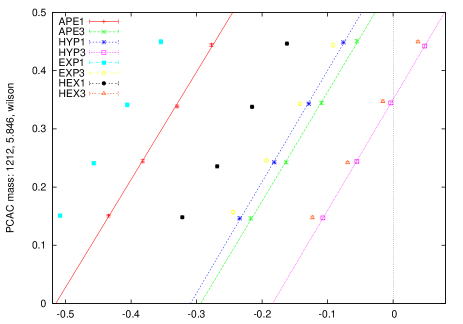
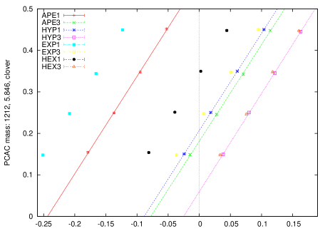
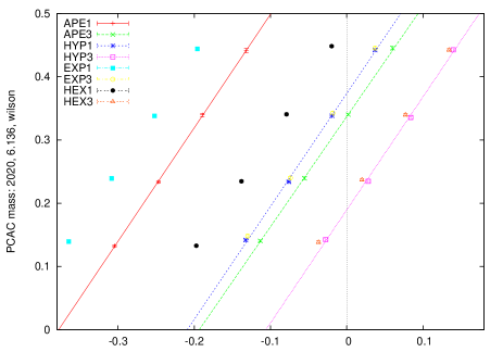
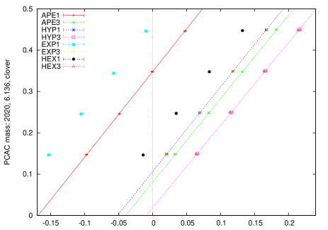
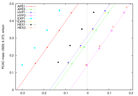
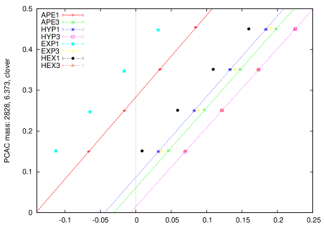
Figure 2: Our data for $2m^{\mathrm{PCAC}}$ vs. $m_{0}$ with $c_{\mathrm{SW}}\!=\!0$ (left) and $c_{\mathrm{SW}}\!=\!1$ (right) at three couplings.

For clover fermions one has, up to $O(ag_{0}^{2},...,a^{2})$ terms, the vector and axial-vector Ward identities

$$Z_{V}\langle.|\bar{\partial}_{\mu}\tilde{V}_{\mu}^{a}(x)|.\rangle\! \!=\! \!{Z_{m}(a\mu)Z_{S}(a\mu)\over 4}(\tilde{m}_{2}^{\mathrm{W}}\!-\!\tilde{m}_{1}^{\mathrm{W}})\langle.|\tilde{S}^{a}(x\!+\!\hat{4})+\!2\tilde{S}^{a}(x)+\!\tilde{S}^{a}(x\!-\!\hat{4})|.\rangle\quad$$ (17)

$$Z_{A}\langle.|\bar{\partial}_{\mu}\tilde{A}_{\mu}^{a}(x)|.\rangle\! \!=\! \!{Z_{m}(a\mu)Z_{P}(a\mu)\over 4}(\tilde{m}_{2}^{\mathrm{W}}\!+\!\tilde{m}_{1}^{\mathrm{W}})\langle.|\tilde{P}^{a}(x\!+\!\hat{4})\!+\!2\tilde{P}^{a}(x)\!+\!\tilde{P}^{a}(x\!-\!\hat{4})|.\rangle\quad$$ (18)

with $\tilde{m}^{W}\!=\!(1\!+\!b_{m}am^{\mathrm{W}})m^{\mathrm{W}}$. The unmixed densities/currents $\tilde{X}$ with $X\!=\!S,P,V,A$ have been given in (12). Note that either r.h.s. is scale-independent, since $Z_{m}\!=\!1/Z_{S}$ and the two renormalization factors $Z_{S}$ and $Z_{P}$ run synchronously. Finally, due to the $b_{m}$ term in (14), $m_{\mathrm{crit}}$ does not drop out of the r.h.s. of (17) for unequal current quark masses.

A naive determination of $-am_{\mathrm{crit}}\!=\!4-1/(2\kappa_{\mathrm{crit}})$ would measure $M_{\pi}^{2}$ as a function of $m_{0}$ and determine, via an extrapolation, where the former vanishes. To avoid finite-volume and/or chiral log effects, we determine $m^{\mathrm{PCAC}}$ as a function of $m_{0}$ and see where this quantity vanishes. Up to $O(ag_{0}^{2},...,a^{2})$ [depending on the details of improvement] cut-off effects this is a linear relationship, and, by virtue of (18), the slope is proportional to $Z_{m}Z_{P}/Z_{A}$. More specifically, we restrict ourselves to degenerate quark masses (i.e. $m_{1}\!=\!m_{2}$) and employ the fitting ansatz

$$am^{\mathrm{PCAC}}={1\over\tilde{Z}_{A}}\,[1+b_{m}(am_{0}-am_{\mathrm{crit}})](am_{0}-am_{\mathrm{crit}})$$ (19)

with $m_{0}$ the bare fermion mass given in (13). The goal is to test how well the fitted $-am_{\mathrm{crit}}$ and $\tilde{Z}_{A}\!=\!Z_{A}/(Z_{m}Z_{P})$ agree with the 1-loop prediction. In principle, the coefficient $b_{m}$ is known at tree level. It turns out that using this value leads to unacceptable fits. On the other hand, our data are not precise enough to allow us to use $b_{m}$ as a parameter. The quoted fits use $b_{m}\!=\!0$; this leads in most cases to acceptable chisquares, and the few exceptions might be due to our limited statistics (cf. Tab. 7). In fact, our data (taken at fixed $am^{\mathrm{PCAC}}$ to limit the CPU requirements) do not show any visible curvature – Fig. 2 shows the data for three (out of five) couplings. We performed several alternative fits (e.g. by dropping the last data point), and as a result we estimate that the theoretical uncertainty is roughly one order of magnitude larger than the statistical error quoted in Tabs. 9-11.

$c_{\mathrm{SW}}\!=\!0$	$\beta=5.846$	$\beta=6.000$	$\beta=6.136$	$\beta=6.260$	$\beta=6.373$
thin link	0.44573	0.43429	0.42466	0.41625	0.40887
pert.	0.11750	0.11448	0.11194	0.10973	0.10778
1 APE	0.5150(18)	0.4283(17)	0.3779(17)	0.3496(22)	0.3248(15)
1 EXP	0.5846(23)	0.4932(15)	0.4412(21)	0.4039(11)	0.3805(09)
pert.	0.04170	0.04063	0.03973	0.03894	0.03825
3 APE	0.2939(20)	0.2247(16)	0.1935(14)	0.1685(16)	0.1555(17)
3 EXP	0.3263(21)	0.2509(18)	0.2100(19)	0.1869(08)	0.1713(19)
pert.	0.06046	0.05891	0.05760	0.05646	0.05546
1 HYP	0.3094(18)	0.2455(14)	0.2093(16)	0.1908(15)	0.1728(28)
1 HEX	0.3985(19)	0.3158(18)	0.2715(12)	0.2449(16)	0.2244(06)
pert.	—	—	—	—	—
3 HYP	0.1841(18)	0.1290(14)	0.1061(11)	0.0949(17)	0.0794(15)
3 HEX	0.1993(18)	0.1419(14)	0.1142(16)	0.0976(14)	0.0868(16)

Table 8: For $c_{\mathrm{SW}}\!=\!0$ Wilson fermions: $-am_{\mathrm{crit}}$ with 8 filtering recipes. In each field, the first row gives the (common) 1-loop prediction, and the next two the linearly extrapolated values with APE/EXP or HYP/HEX filtering, respectively. Errors are statistical only. We did not measure the unfiltered $-am_{\mathrm{crit}}$, and we do not have a perturbative prediction for 3 HYP/HEX steps.

$c_{\mathrm{SW}}\!=\!1$	$\beta=5.846$	$\beta=6.000$	$\beta=6.136$	$\beta=6.260$	$\beta=6.373$
thin link	0.27719	0.27008	0.26409	0.25886	0.25427
pert.	0.04254	0.04145	0.04053	0.03973	0.03902
1 APE	0.2438(13)	0.1929(08)	0.1685(07)	0.1518(08)	0.1413(05)
1 EXP	0.3140(13)	0.2547(11)	0.2231(08)	0.2022(06)	0.1873(04)
pert.	0.00668	0.00651	0.00637	0.00624	0.00613
3 APE	0.0779(13)	0.0497(07)	0.0400(04)	0.0341(02)	0.0312(03)
3 EXP	0.1003(13)	0.0657(07)	0.0512(06)	0.0440(03)	0.0392(02)
pert.	0.01719	0.01675	0.01638	0.01605	0.01577
1 HYP	0.0885(10)	0.0620(05)	0.0517(05)	0.0475(03)	0.0441(03)
1 HEX	0.1464(14)	0.1045(07)	0.0851(04)	0.0743(03)	0.0674(04)
pert.	—	—	—	—	—
3 HYP	0.0252(12)	0.0120(05)	0.0094(02)	0.0084(01)	0.0077(03)
3 HEX	0.0289(10)	0.0143(05)	0.0111(04)	0.0088(02)	0.0088(02)

Table 9: For $c_{\mathrm{SW}}\!=\!1$ clover fermions: $-am_{\mathrm{crit}}$ with 8 filtering recipes (cf. caption of Tab. 9).

Our non-perturbative data for $-am_{\mathrm{crit}}$ are given in Tab. 9 and Tab. 9 for the Wilson ($c_{\mathrm{SW}}\!=\!0$) and clover ($c_{\mathrm{SW}}\!=\!1$) case, respectively. As an illustration, we add the 1-loop prediction that follows from (5, 13) and Tab. 1. We did not measure the unfiltered $-am_{\mathrm{crit}}$, since it would be too expensive for our computational resources, and the large discrepancy between the perturbative and non-perturbative critical mass for unfiltered actions is well known.

$c_{\mathrm{SW}}\!=\!0$	$\beta=5.846$	$\beta=6.000$	$\beta=6.136$	$\beta=6.260$	$\beta=6.373$
thin link	0.94668	0.94805	0.94920	0.95020	0.95109
pert.	0.99859	0.99863	0.99866	0.99868	0.99871
1 APE	1.081(12)	1.115(11)	1.115(12)	1.134(16)	1.132(09)
1 EXP	1.037(16)	1.086(11)	1.110(13)	1.095(08)	1.121(10)
pert.	1.00281	1.00274	1.00268	1.00262	1.00258
3 APE	1.066(13)	1.114(11)	1.149(10)	1.123(10)	1.130(10)
3 EXP	1.067(14)	1.132(12)	1.117(12)	1.120(05)	1.140(10)
pert.	1.00061	1.00059	1.00058	1.00057	1.00056
1 HYP	1.046(12)	1.129(09)	1.120(10)	1.137(09)	1.114(14)
1 HEX	1.070(12)	1.117(12)	1.126(08)	1.139(09)	1.129(07)
pert.	—	—	—	—	—
3 HYP	1.051(11)	1.113(09)	1.119(08)	1.148(11)	1.114(10)
3 HEX	1.058(11)	1.119(09)	1.125(10)	1.125(10)	1.119(09)

Table 10: For $c_{\mathrm{SW}}\!\!=\!0$ Wilson fermions: $Z_{A}/(Z_{m}Z_{P})$ with 8 filtering recipes (cf. caption of Tab. 9).

$c_{\mathrm{SW}}\!=\!1$	$\beta=5.846$	$\beta=6.000$	$\beta=6.136$	$\beta=6.260$	$\beta=6.373$
thin link	0.90710	0.90949	0.91149	0.91324	0.91478
pert.	0.98030	0.98080	0.98123	0.98160	0.98193
1 APE	0.8523(86)	0.9263(55)	0.9679(51)	0.9798(70)	0.9974(42)
1 EXP	0.8602(80)	0.9477(44)	0.9912(26)	1.0079(17)	1.0200(24)
pert.	0.99424	0.99439	0.99451	0.99462	0.99472
3 APE	0.8554(69)	0.9398(33)	0.9761(31)	1.0008(22)	1.0126(24)
3 EXP	0.8458(80)	0.9503(28)	1.0024(15)	1.0258(10)	1.0340(21)
pert.	0.99014	0.99040	0.99061	0.99080	0.99096
1 HYP	0.8539(88)	0.9195(72)	0.9599(51)	0.9699(49)	0.9847(37)
1 HEX	0.8703(78)	0.9510(42)	0.9841(34)	1.0039(25)	1.0160(15)
pert.	—	—	—	—	—
3 HYP	0.8517(93)	0.9435(42)	0.9713(33)	0.9959(23)	1.0074(28)
3 HEX	0.8452(61)	0.9548(30)	1.0050(26)	1.0193(13)	1.0373(11)

Table 11: For $c_{\mathrm{SW}}\!=\!1$ clover fermions: $Z_{A}/(Z_{m}Z_{P})$ with 8 filtering recipes (cf. caption of Tab. 9).

Our non-perturbative data for $\tilde{Z}_{A}$ are given in Tab. 11 and Tab. 11 for the cases $c_{\mathrm{SW}}\!=\!0$ and $c_{\mathrm{SW}}\!=\!1$, respectively. Note that $\tilde{Z}_{A}$ is scale-independent, since $Z_{m}\!=\!1/Z_{S}$, and the factors $Z_{S}$ and $Z_{P}$ run synchronously. Again, we add the 1-loop prediction that follows from (7) and Tabs. 4 - 4. For similar reasons as above, we did not measure the unfiltered $\tilde{Z}_{A}$.

The overall impression from Tabs. 9-11 is that 1-loop perturbation theory does not give very accurate predictions for non-perturbatively determined renormalization factors, if the improvement coefficients are taken at tree-level. However, the mismatch is much smaller if filtering and improvement is used – as soon as one of the ingredients is missing, the “agreement” gets much worse. The virtue of the combined “filtering and improvement” program is that all renormalization factors and improvement coefficients are close to their respective tree-level values. This is in marked contrast to other schemes (e.g. [16]) in which these quantities are far from $0$ and $1$, respectively, and the challenge is to reproduce these big numbers in perturbation theory.

4.2 Rational fits for $m_{\mathrm{crit}}$ with APE/HYP/EXP/HEX filtering

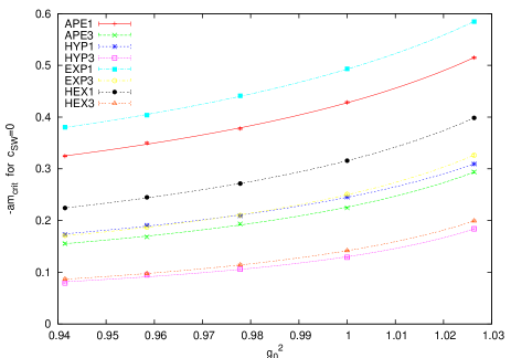
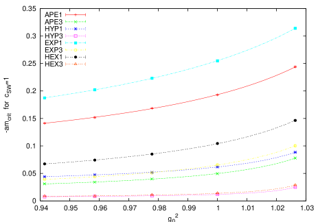
Figure 3: $-am_{\mathrm{crit}}$ vs. $g_{0}^{2}$ for Wilson ($c_{\mathrm{SW}}\!=\!0$, left) and clover ($c_{\mathrm{SW}}\!=\!1$, right) fermions with 8 filterings. The curves indicate 3-parameter rational fits.

		$c_{\mathrm{SW}}=0$		$c_{\mathrm{SW}}=1$
pert.		0.114480		0.0414467
1 APE	1 EXP	0.213(12)	0.252(12)	0.0909(28)	0.1094(20)
pert.		0.040629		0.0065096
3 APE	3 EXP	0.077(14)	0.083(07)	0.0172(15)	0.0171(09)
pert.		0.058906		0.0167502
1 HYP	1 HEX	0.095(14)	0.121(04)	0.0338(12)	0.0332(16)
pert.		—		—
3 HYP	3 HEX	0.034(15)	0.026(01)	0.0060(02)	0.0060(15)

Table 12: The fitted coefficient $c_{1}$ in (20), compared with the 1-loop prediction $S/(12\pi^{2})$ with $S$ taken from Tab. 1.

We know from (5) that asymptotically $-am_{\mathrm{crit}}\to g_{0}^{2}S/(12\pi^{2})=S/(2\pi^{2}\beta)$ with $S$ given in Tab. 1. Accordingly, if we fit our data with the rational ansatz

$$-am_{\mathrm{crit}}={c_{1}g_{0}^{2}+c_{2}g_{0}^{4}\over 1+c_{3}g_{0}^{2}}$$ (20)

then the coefficient $c_{1}$ would correspond, in the weak coupling regime, to $S/(12\pi^{2})$ with $S$ given in Tab. 1. Our data are not in the weak coupling regime, but still it is interesting to check how much the coefficient $c_{1}$ from an unconstrained fit deviates from the perturbative value. The result is shown in Fig. 3 and Tab. 12. As was to be anticipated from our discussion of Tabs.9-9, the “agreement” is not very good. On an absolute scale the numbers are close, since they are all much smaller than one. On a relative scale, they deviate by a substantial factor. In spite of this disagreement, the non-perturbative data still show a consistency $c_{1}^{\mathrm{APE}}\!\simeq\!c_{1}^{\mathrm{EXP}}$ and ditto for $c_{1}^{\mathrm{HYP}}\!\simeq\!c_{1}^{\mathrm{HEX}}$, as predicted in PT. We find this amusing, in particular in view of the fact that the corresponding (in PT) curves in Fig. 3 are not close at all.

4.3 Rational fits for $\tilde{Z}_{A}$ with APE/HYP/EXP/HEX filtering

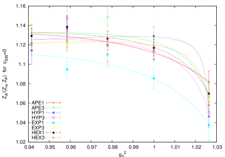
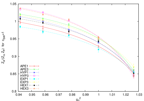
Figure 4: $Z_{A}/(Z_{m}Z_{P})$ vs. $g_{0}^{2}$ for Wilson ($c_{\mathrm{SW}}\!=\!0$, left) and clover ($c_{\mathrm{SW}}\!=\!1$, right) fermions with 8 filterings. The curves indicate 3-parameter rational fits.

We know from (7) that asymptotically $\tilde{Z}_{A}\to 1\!-\!g_{0}^{2}(z_{A}\!+\!z_{S}\!-\!z_{P})/(12\pi^{2})=1\!-\!(z_{A}\!+\!z_{S}\!-\!z_{P})/(2\pi^{2}\beta)$. Accordingly, if we fit our data with the rational ansatz

$$\tilde{Z}_{A}={1+d_{1}g_{0}^{2}+d_{2}g_{0}^{4}\over 1+d_{3}g_{0}^{2}}$$ (21)

then $d_{1}\!-\!d_{3}$ would correspond, in the weak coupling regime, to $(z_{A}\!+\!z_{S}\!-\!z_{P})/(12\pi^{2})$ with $z_{A},z_{S},z_{P}$ given in Tabs. 4 - 4. The result of our fits is displayed in Fig. 4. Again, there is no quantitative agreement between 1-loop perturbation theory for $\tilde{Z}_{A}$ and our non-perturbative data, based on tree-level improvement coefficients. Still, comparing the two graphs in Fig. 4, one is led to believe that with appropriate 1-loop improvement coefficients the situation might be better.

4.4 Rational fits for $m_{\mathrm{res}}$ with APE/HYP/EXP/HEX filtering

We may express our result in terms of $m_{\mathrm{res}}\!=\!m^{\mathrm{PCAC}}(m_{0}\!=\!0)$. $\tilde{Z}_{A}\!\simeq\!1$ implies $m_{\mathrm{res}}\!\simeq\!-m_{\mathrm{crit}}$, and we refrain from copying Tabs. 9-9 with minimal modifications. Again, we performed rational fits, and the result looks very similar to Fig. 3. An interesting observation is that $m_{\mathrm{res}}$ in physical units is almost constant. We find $m_{\mathrm{res}}^{\mathrm{3\,APE}}\!\simeq\!144,111,107,108,113\,\mathrm{MeV}$ at $\beta\!=\!5.846,6.0,6.136,6.260,6.373$ and $m_{\mathrm{res}}^{\mathrm{3\,HYP}}\!\simeq\!47,27,25,26,27\,\mathrm{MeV}$. We feel confident that with 1-loop values for the coefficients $c_{\mathrm{SW}},c_{A},b_{A}\!-\!b_{P}$ smaller residual masses could be obtained.

5 Summary

We have presented a systematic study of filtered Wilson and clover quarks in quenched QCD. We have derived results at 1-loop order in weak-coupling perturbation theory for $-am_{\mathrm{crit}}$ and the renormalization factors $Z_{X}$ with $X\!=\!S,P,V,A$ with four filterings [APE, HYP, EXP, HEX], in some cases with 1,2,3 iterations. We have compared these predictions to non-perturbative data for $-am_{\mathrm{crit}}$ and $\tilde{Z}_{A}\!=\!Z_{A}Z_{S}/Z_{P}$ in a simulation without improvement and with tree-level improvement coefficients. We find no quantitative agreement in this specific setup. Still, the tremendous progress that comes through the combination of tree-level improvement and filtering leaves us optimistic that a theory with 1-loop improvement coefficients and 2-loop renormalization factors might work in practice. By this we mean that a continuum extrapolation can be done from accessible couplings as if the theory would have $O(a^{2})$ cut-off effects only.

It turns out that lattice perturbation theory for UV-filtered fermion actions is not much more complicated than for unfiltered actions. For instance, our formula (73) gives a compact 1-loop expression for the critical mass with an arbitrary number of APE smearings, and shows that $am_{\mathrm{crit}}\to 0$ for $n_{\mathrm{iter}}\to\infty$. Since our results in the main part of the article were derived in a fully automated manner, we feel that this explicit calculation provides an important check.

One particularly compelling feature of filtered clover actions is that tadpole resummation is not needed; in fact it barely changes the result. This suggests that perturbation theory for filtered clover quarks converges well. In consequence, we expect that for filtered clover fermions the non-perturbative improvement conditions as implemented by the ALPHA collaboration [15] will yield values consistent with such perturbative predictions.

A beneficial feature in phenomenological applications is the low noise in observables built from filtered clover quarks. We have been able to determine $m_{\mathrm{crit}}$ to $\sim\!3\%$ statistical accuracy from just a handful of configurations. Therefore, the “filtering” comes at no cost – it actually reduces the CPU time needed to obtain a predefined accuracy in the continuum limit.

Let us comment on the filtering in two different fermion formulations. It is clear that twisted-mass Wilson fermions would benefit from filtering, too. The dramatic renormalization of the twist angle would be tamed and it would be much easier to realize maximum (renormalized) twist. For rather different technical reasons, filtering has proven useful for overlap fermions [18, 29, 30]. In our technical study we decided to stay with $c_{\mathrm{SW}}\!=\!0$, because the overlap prescription achieves automatic $O(a)$ on-shell improvement. It is not clear to us whether the better chiral properties of a clover kernel could translate into further savings in the overlap construction.

We hope that, once the 1-loop value for $c_{\mathrm{SW}}$ with $n$ iterations of the EXP/stout recipe [20] is known, filtered clover fermions are ready for use in large-scale dynamical simulations. An important point is, of course, the smallest valence quark mass that can be reached for a given coupling and sea quark mass (partially quenched setup). We find $am_{\mathrm{res}}^{\mathrm{3\,HYP}}\!=\!0.0126(5)$ at $\beta\!=\!6.0$ and $am_{\mathrm{res}}^{\mathrm{3\,HYP}}\!=\!0.0074(3)$ at $\beta\!=\!6.373$ in the quenched theory. This corresponds to an almost constant residual mass in physical units, $m_{\mathrm{res}}^{\mathrm{3\,HYP}}\!\simeq\!27\,\mathrm{MeV}$. Since this mass is much smaller than in the unfiltered case, it is natural to hope that one can reach smaller valence quark masses (in the quenched or partially quenched setup) before one runs into the problem of “exceptional” configurations. Furthermore, if mixing with unwanted chiralities in 4-fermi operators is an $O((am_{\mathrm{res}})^{2})$ effect [31] in our case, too, the small residual mass would be relevant for electroweak phenomenology. Clearly, these topics deserve detailed investigations.

Acknowledgments

We thank Tom DeGrand for useful correspondence. S.D. is indebted to Ferenc Niedermayer for discussions on fat-link actions. S.D. was supported by the Swiss NSF, S.C. by the Fonds zur Förderung der Wissenschaftlichen Forschung in Österreich (FWF), Project P16310-N08.

Appendix A Fat link perturbation theory in $d$ dimensions

A.1 APE smearing

In $d$ dimensions and with general gauge group $G$, standard APE smearing is defined through

$$U_{\mu}^{\prime}(x)=P_{G}\Big{\{}\,(1\!-\!\alpha)U_{\mu}(x)+{\alpha\over 2(d\!-\!1)}\sum_{\pm\nu\neq(\mu)}U_{\nu}(x)\,U_{\mu}(x\!+\!\hat{\nu})\,U_{\nu}(x\!+\!\hat{\mu})^{\dagger}\Big{\}}$$

where the sum (“staple”) includes $2(d\!-\!1)$ terms. The projection $P_{G}$ is needed, since in general the staple is no longer a group element. For the perturbative expansion we substitute $U_{\mu}(x)\to 1+\mathrm{i}aA_{\mu}(x\!+\!{\hat{\mu}\over 2})+O(a^{2})$. The prefactors $1\!-\!\alpha,\alpha/(2d\!-\!2)$ ensure that in PT the effect of $P_{G}$ is already taken care of. For 2-quark and 4-quark renormalization factors at 1-loop order only the linear part is relevant [11]. After shifting $x\to x\!-\!{\hat{\mu}\over 2}$ one obtains at leading order

$$A_{\mu}^{\prime}(x) = A_{\mu}(x)\;+\;{\alpha\over 2(d\!-\!1)}\sum_{\nu}\Big{\{}A_{\mu}(x\!+\hat{\nu})-2A_{\mu}(x)+A_{\mu}(x\!-\hat{\nu})\Big{\}}$$ (22)

$$+ {\alpha\over 2(d\!-\!1)}\sum_{\nu}\Big{\{}A_{\nu}(x\!-\!{\hat{\mu}\over 2}\!+\!{\hat{\nu}\over 2})-A_{\nu}(x\!-\!{\hat{\mu}\over 2}\!-\!{\hat{\nu}\over 2})-A_{\nu}(x\!+\!{\hat{\mu}\over 2}\!+\!{\hat{\nu}\over 2})+A_{\nu}(x\!+\!{\hat{\mu}\over 2}\!-\!{\hat{\nu}\over 2})\Big{\}}\quad$$

where the sum now extends over all positive $\nu$. This may be recast into the form

$$\omega(y) = \delta_{y,0}+{\alpha\over 2(d\!-\!1)}\sum_{\rho}\,\{\delta_{y,\hat{\rho}}-2\delta_{y,0}+\delta_{y,-\hat{\rho}}\}$$

$$\omega_{\mu\nu}(y) = {\alpha\over 2(d\!-\!1)}\Big{[}\delta_{y,-{\hat{\mu}\over 2}+{\hat{\nu}\over 2}}-\delta_{y,-{\hat{\mu}\over 2}-{\hat{\nu}\over 2}}-\delta_{y,+{\hat{\mu}\over 2}+{\hat{\nu}\over 2}}+\delta_{y,+{\hat{\mu}\over 2}-{\hat{\nu}\over 2}}\Big{]}$$

$$A_{\mu}^{\prime}(x) = \sum_{y,\nu}\,h_{\mu\nu}(y)\,A_{\nu}(x\!+\!y)=\sum_{y,\nu}\,\Big{\{}[\omega(y)\delta_{\mu,\nu}+\omega_{\mu\nu}(y)]\,A_{\nu}(x\!+\!y)\Big{\}}$$ (23)

which is suitable for a Fourier transformation. This leads to the final relation

$$A_{\mu}^{\prime}(q) = \sum\limits_{\nu}\,\Big{\{}\Big{(}[1-{\alpha\over 2(d\!-\!1)}\hat{q}^{2}]\delta_{\mu,\nu}+{\alpha\over 2(d\!-\!1)}\hat{q}_{\mu}\hat{q}_{\nu}\Big{)}\,A_{\nu}(q)\Big{\}}$$ (24)

$$= [1-{\alpha\over 2(d\!-\!1)}(\hat{q}^{2}\!-\!\hat{q}_{\mu}^{2})]\,A_{\mu}(q)+{\alpha\over 2(d\!-\!1)}\sum\limits_{\nu\neq(\mu)}\Big{\{}\hat{q}_{\mu}\hat{q}_{\nu}A_{\nu}(q)\Big{\}}$$

$$= A_{\mu}(q)+{\alpha\over 2(d\!-\!1)}\sum\limits_{\nu\neq(\mu)}\,\Big{\{}-\hat{q}_{\nu}^{2}A_{\mu}(q)+\hat{q}_{\mu}\hat{q}_{\nu}A_{\nu}(q)\Big{\}}$$

with $\hat{q}_{\rho}={2\over a}\sin({a\over 2}q_{\rho})$ (for all $d$). A form particularly useful for iterated smearing ($n\!>\!1$) is [11]

$$A_{\mu}^{(n)}(q)=\sum_{\nu}\,\Big{\{}\Big{(}[1-{\alpha\over 2(d\!-\!1)}\hat{q}^{2}]^{n}\,(\delta_{\mu,\nu}-{\hat{q}_{\mu}\hat{q}_{\nu}\over\hat{q}^{2}})+{\hat{q}_{\mu}\hat{q}_{\nu}\over\hat{q}^{2}}\Big{)}\,A_{\nu}(q)\Big{\}}$$ (25)

where the transverse part is simply a form-factor $f^{(n)}({\hat{q}}^{2})=[1-{\alpha\over 2(d\!-\!1)}\hat{q}^{2}]^{n}$ as emphasized in [11].

A.2 HYP smearing

In $d\!\geq\!3$ dimensions $d\!-\!1$ levels of restricted APE smearings may be nested in such a way that the final “fat” link contains only “thin” links in the adjacent hypercubes [9]. Specifically, in $d\!=\!4$ the linearized HYP relation reads (note that $\alpha_{3,2,1}$ refer to step 1,2,3, respectively)

$$\bar{A}_{\mu,\nu\rho}(x) = (1-\alpha_{3})A_{\mu}(x)+{\alpha_{3}\over 2}\sum_{\pm\sigma\neq(\mu\nu\rho)}\Big{\{}A_{\sigma}(x\!-\!{\hat{\mu}\over 2}\!+\!{\hat{\sigma}\over 2})+A_{\mu}(x\!+\!\sigma)+A_{\sigma}(x\!+\!{\hat{\mu}\over 2}\!+\!{\hat{\sigma}\over 2})\Big{\}}$$

$$\tilde{A}_{\mu,\nu}(x) = (1-\alpha_{2})A_{\mu}(x)+{\alpha_{2}\over 4}\sum_{\pm\rho\neq(\mu\nu)}\Big{\{}\bar{A}_{\rho,\mu\nu}(x\!-\!{\hat{\mu}\over 2}\!+\!{\hat{\rho}\over 2})+\bar{A}_{\mu,\nu\rho}(x\!+\!\rho)+\bar{A}_{\rho,\mu\nu}(x\!+\!{\hat{\mu}\over 2}\!+\!{\hat{\rho}\over 2})\Big{\}}$$

$$A_{\mu}^{\prime}(x) = (1-\alpha_{1})A_{\mu}(x)+{\alpha_{1}\over 6}\sum_{\pm\nu\neq(\mu)}\Big{\{}\tilde{A}_{\nu,\mu}(x\!-\!{\hat{\mu}\over 2}\!+\!{\hat{\nu}\over 2})+\tilde{A}_{\mu,\nu}(x\!+\!\nu)+\tilde{A}_{\nu,\mu}(x\!+\!{\hat{\mu}\over 2}\!+\!{\hat{\nu}\over 2})\Big{\}}$$

and it is easy to see that the core recipe in each step is an APE smearing in 2,3,4 dimensions, respectively. Therefore, the Fourier transform leads to the relations

$$\bar{A}_{\mu,\nu\rho}(q) = A_{\mu}(q)+{\alpha_{3}\over 2}\sum_{\sigma\neq(\mu\nu\rho)}\Big{\{}-\hat{q}_{\sigma}^{2}A_{\mu}(q)+\hat{q}_{\mu}\hat{q}_{\sigma}A_{\sigma}(q)\Big{\}}$$

$$\tilde{A}_{\mu,\nu}(q) = (1-\alpha_{2})A_{\mu}(q)+{\alpha_{2}\over 4}\sum_{\rho\neq(\mu\nu)}\Big{\{}(2-\hat{q}_{\rho}^{2})\bar{A}_{\mu,\nu\rho}(q)+\hat{q}_{\mu}\hat{q}_{\rho}\bar{A}_{\rho,\mu\nu}(q)\Big{\}}$$

$$A_{\mu}^{\prime}(q) = (1-\alpha_{1})A_{\mu}(q)+{\alpha_{1}\over 6}\sum_{\nu\neq(\mu)}\Big{\{}(2-\hat{q}_{\nu}^{2})\tilde{A}_{\mu,\nu}(q)+\hat{q}_{\mu}\hat{q}_{\nu}\tilde{A}_{\nu,\mu}(q)\Big{\}}$$ (26)

where a simplification specific to the innermost level has been applied. Plugging everything in we obtain a compact momentum space representation for one level of HYP smearing

$$A_{\mu}^{\prime} = A_{\mu}+{\alpha_{1}\over 6}\sum_{\nu\neq(\mu)}\Big{\{}{\hat{q}}_{\mu}{\hat{q}}_{\nu}A_{\nu}-{\hat{q}}_{\nu}^{2}A_{\mu}+{\alpha_{2}\over 4}\sum_{\rho\neq(\mu\nu)}\Big{\{}2{\hat{q}}_{\mu}{\hat{q}}_{\rho}A_{\rho}-{\hat{q}}_{\rho}^{2}[(2-{\hat{q}}_{\nu}^{2})A_{\mu}+{\hat{q}}_{\mu}{\hat{q}}_{\nu}A_{\nu}]+$$ (27)

$${\alpha_{3}\over 2}\sum_{\sigma\neq(\mu\nu\rho)}\Big{\{}4{\hat{q}}_{\mu}{\hat{q}}_{\sigma}A_{\sigma}-{\hat{q}}_{\sigma}^{2}[2{\hat{q}}_{\mu}{\hat{q}}_{\rho}A_{\rho}+(2-{\hat{q}}_{\rho}^{2})[(2-{\hat{q}}_{\nu}^{2})A_{\mu}+{\hat{q}}_{\mu}{\hat{q}}_{\nu}A_{\nu}]]\Big{\}}\Big{\}}\Big{\}}$$

which, however, entails some orthogonality constraints. To get rid of the latter, we apply a number of tricks. First, the sum over $\sigma$ is split into two parts. The part quadratic in ${\hat{q}}_{\sigma}$ can be made independent of the summation index by virtue of ${\hat{q}}_{\sigma}^{2}={\hat{q}}^{2}-{\hat{q}}_{\mu}^{2}-{\hat{q}}_{\nu}^{2}-{\hat{q}}_{\rho}^{2}$. Hence, what remains in the innermost summation is the term linear in ${\hat{q}}_{\sigma}$. This term, however, is independent of $\rho$, the next-level index. Since the constraint lets it assume the other free value (after $\mu$ and $\nu$ have been fixed) than $\rho$, the total effect is the same as with $\sigma\!\to\!\rho$ replaced, thus

$$A_{\mu}^{\prime} = A_{\mu}+{\alpha_{1}\over 6}\sum_{\nu\neq(\mu)}\Big{\{}{\hat{q}}_{\mu}{\hat{q}}_{\nu}A_{\nu}-{\hat{q}}_{\nu}^{2}A_{\mu}+{\alpha_{2}\over 4}\sum_{\rho\neq(\mu\nu)}\Big{\{}(2\!+\!\alpha_{3}(2-{\hat{q}}^{2}+{\hat{q}}_{\mu}^{2}+{\hat{q}}_{\nu}^{2}+{\hat{q}}_{\rho}^{2})){\hat{q}}_{\mu}{\hat{q}}_{\rho}A_{\rho}$$

$$-[{\hat{q}}_{\rho}^{2}+{\alpha_{3}\over 2}({\hat{q}}^{2}-{\hat{q}}_{\mu}^{2}-{\hat{q}}_{\nu}^{2}-{\hat{q}}_{\rho}^{2})(2-{\hat{q}}_{\rho}^{2})][(2-{\hat{q}}_{\nu}^{2})A_{\mu}+{\hat{q}}_{\mu}{\hat{q}}_{\nu}A_{\nu}]\Big{\}}\Big{\}}$$

is a representation with only two sums. Next we pull out those parts which are independent of the index $\rho$. Using $\sum_{\rho\neq(\mu\nu)}{\hat{q}}_{\rho}^{2}={\hat{q}}^{2}-{\hat{q}}_{\mu}^{2}-{\hat{q}}_{\nu}^{2}$ in the remainder yields

$$A_{\mu}^{\prime} = A_{\mu}+{\alpha_{1}\over 6}\sum_{\nu\neq(\mu)}\Big{\{}{\hat{q}}_{\mu}{\hat{q}}_{\nu}A_{\nu}-{\hat{q}}_{\nu}^{2}A_{\mu}+{\alpha_{2}\over 4}\sum_{\rho\neq(\mu\nu)}\Big{\{}(2\!+\!\alpha_{3}(2-{\hat{q}}^{2}+{\hat{q}}_{\mu}^{2}+{\hat{q}}_{\nu}^{2}+{\hat{q}}_{\rho}^{2})){\hat{q}}_{\mu}{\hat{q}}_{\rho}A_{\rho}\Big{\}}$$

$$-{\alpha_{2}\over 4}[(1\!+\!\alpha_{3})({\hat{q}}^{2}-{\hat{q}}_{\mu}^{2}-{\hat{q}}_{\nu}^{2})-{\alpha_{3}\over 2}[({\hat{q}}^{2}-{\hat{q}}_{\mu}^{2}-{\hat{q}}_{\nu}^{2})^{2}-\sum_{\rho\neq(\mu\nu)}{\hat{q}}_{\rho}^{4}]][(2-{\hat{q}}_{\nu}^{2})A_{\mu}+{\hat{q}}_{\mu}{\hat{q}}_{\nu}A_{\nu}]\Big{\}}$$

where the bracket multiplying ${\alpha_{3}\over 2}$ is just $2\prod_{\rho\neq(\mu\nu)}{\hat{q}}_{\rho}^{2}$. Since a constrained product would be inconvenient for later use, we choose to stay with the actual form, but now we relax the constraint on $\rho$ to differ from $\mu$ only and compensate for the additional term. This yields

$$A_{\mu}^{\prime} = A_{\mu}+{\alpha_{1}\over 6}\sum_{\nu\neq(\mu)}\Big{\{}[1-{\alpha_{2}\over 4}(2+\alpha_{3}(2-{\hat{q}}^{2}+{\hat{q}}_{\mu}^{2}+2{\hat{q}}_{\nu}^{2}))]{\hat{q}}_{\mu}{\hat{q}}_{\nu}A_{\nu}-{\hat{q}}_{\nu}^{2}A_{\mu}$$

$$-{\alpha_{2}\over 4}[(1+\alpha_{3})({\hat{q}}^{2}-{\hat{q}}_{\mu}^{2}-{\hat{q}}_{\nu}^{2})-{\alpha_{3}\over 2}Q_{\mu\nu}][(2-{\hat{q}}_{\nu}^{2})A_{\mu}+{\hat{q}}_{\mu}{\hat{q}}_{\nu}A_{\nu}]$$

$$+{\alpha_{2}\alpha_{3}\over 4}{\hat{q}}_{\nu}^{2}\sum_{\rho\neq(\mu)}\Big{\{}{\hat{q}}_{\mu}{\hat{q}}_{\rho}A_{\rho}\Big{\}}+{\alpha_{2}\over 4}\sum_{\rho\neq(\mu)}\Big{\{}(2\!+\!\alpha_{3}(2-{\hat{q}}^{2}+{\hat{q}}_{\mu}^{2}+{\hat{q}}_{\rho}^{2})){\hat{q}}_{\mu}{\hat{q}}_{\rho}A_{\rho}\Big{\}}\Big{\}}$$

with $Q_{\mu\nu}=({\hat{q}}^{2}-{\hat{q}}_{\mu}^{2}-{\hat{q}}_{\nu}^{2})^{2}-\sum_{\rho\neq(\mu\nu)}{\hat{q}}_{\rho}^{4}$. In the sum over $\rho$ the term which depends on $\nu$ has been isolated. The reason is that the other term may be pulled out of the $\nu$-sum (this yields a factor 3), and since the constraint is the same, renaming the index $\rho\!\to\!\nu$ is then legal. Applying a similar procedure to the $\nu$-independent factor of the former term, we obtain the form

$$A_{\mu}^{\prime} = A_{\mu}+{\alpha_{1}\over 6}\sum_{\nu\neq(\mu)}\Big{\{}[1+\alpha_{2}(1+{\alpha_{3}\over 4}(4-{\hat{q}}^{2}+{\hat{q}}_{\mu}^{2}+{\hat{q}}_{\nu}^{2}))]{\hat{q}}_{\mu}{\hat{q}}_{\nu}A_{\nu}-{\hat{q}}_{\nu}^{2}A_{\mu}$$

$$-{\alpha_{2}\over 4}[(1+\alpha_{3})({\hat{q}}^{2}-{\hat{q}}_{\mu}^{2}-{\hat{q}}_{\nu}^{2})-{\alpha_{3}\over 2}Q_{\mu\nu}][(2-{\hat{q}}_{\nu}^{2})A_{\mu}+{\hat{q}}_{\mu}{\hat{q}}_{\nu}A_{\nu}]\Big{\}}$$

with just one sum [apart from the $A$-independent $\sum{\hat{q}}_{\rho}^{4}$ in $Q_{\mu\nu}=({\hat{q}}^{2}-{\hat{q}}_{\mu}^{2}-{\hat{q}}_{\nu}^{2})^{2}+{\hat{q}}_{\mu}^{4}+{\hat{q}}_{\nu}^{4}-\sum_{\rho}{\hat{q}}_{\rho}^{4}$]. Now it takes a couple of algebraic manipulations to arrive at the form

$$A_{\mu}^{\prime} = A_{\mu}+{\alpha_{1}\over 6}\sum_{\nu\neq(\mu)}\Big{\{}[1+\alpha_{2}(1+\alpha_{3}-{1\over 4}(1+2\alpha_{3})({\hat{q}}^{2}-{\hat{q}}_{\mu}^{2}-{\hat{q}}_{\nu}^{2})+{\alpha_{3}\over 8}Q_{\mu\nu})]{\hat{q}}_{\mu}{\hat{q}}_{\nu}A_{\nu}-{\hat{q}}_{\nu}^{2}A_{\mu}$$

$$-{\alpha_{2}\over 4}[(1+\alpha_{3})(2{\hat{q}}^{2}-2{\hat{q}}_{\mu}^{2}-2{\hat{q}}_{\nu}^{2})-\alpha_{3}(({\hat{q}}^{2})^{2}-2{\hat{q}}^{2}{\hat{q}}_{\mu}^{2}+2{\hat{q}}_{\mu}^{4}-\sum_{\rho}{\hat{q}}_{\rho}^{4})-(1-\alpha_{3})\times$$

$$({\hat{q}}^{2}-{\hat{q}}_{\mu}^{2}-{\hat{q}}_{\nu}^{2}){\hat{q}}_{\nu}^{2}+{\alpha_{3}\over 2}(({\hat{q}}^{2})^{2}-2{\hat{q}}^{2}{\hat{q}}_{\mu}^{2}-2{\hat{q}}^{2}{\hat{q}}_{\nu}^{2}+2{\hat{q}}_{\mu}^{4}+2{\hat{q}}_{\mu}^{2}{\hat{q}}_{\nu}^{2}+2{\hat{q}}_{\nu}^{4}-\sum_{\rho}{\hat{q}}_{\rho}^{4}){\hat{q}}_{\nu}^{2}]A_{\mu}\Big{\}}$$

which is suitable to do the sum in the terms which are even in $q_{\nu}$. This operation yields

$$A_{\mu}^{\prime} = A_{\mu}+{\alpha_{1}\over 6}\sum_{\nu\neq(\mu)}\Big{\{}[1+\alpha_{2}(1+\alpha_{3}-{1\over 4}(1+2\alpha_{3})({\hat{q}}^{2}-{\hat{q}}_{\mu}^{2}-{\hat{q}}_{\nu}^{2})+{\alpha_{3}\over 8}Q_{\mu\nu})]{\hat{q}}_{\mu}{\hat{q}}_{\nu}A_{\nu}\Big{\}}$$

$$-{\alpha_{1}\over 6}(1+\alpha_{2}(1+\alpha_{3}))({\hat{q}}^{2}-{\hat{q}}_{\mu}^{2})A_{\mu}+{\alpha_{1}\alpha_{2}\over 24}(1+2\alpha_{3})(({\hat{q}}^{2})^{2}-2{\hat{q}}^{2}{\hat{q}}_{\mu}^{2}+2{\hat{q}}_{\mu}^{4}-\sum_{\rho}{\hat{q}}_{\rho}^{4})A_{\mu}$$

$$-{\alpha_{1}\alpha_{2}\alpha_{3}\over 48}((({\hat{q}}^{2})^{2}-2{\hat{q}}^{2}{\hat{q}}_{\mu}^{2}+4{\hat{q}}_{\mu}^{4}-3\sum_{\rho}{\hat{q}}_{\rho}^{4})({\hat{q}}^{2}-{\hat{q}}_{\mu}^{2})+2\sum_{\rho}{\hat{q}}_{\rho}^{6}-2{\hat{q}}_{\mu}^{6})A_{\mu}$$

and upon extending the sum and compensating for the additional term one finds

$$A_{\mu}^{\prime} = A_{\mu}+{\alpha_{1}\over 6}\sum_{\nu}\Big{\{}[1+\alpha_{2}(1+\alpha_{3}-{1\over 4}(1+2\alpha_{3})({\hat{q}}^{2}-{\hat{q}}_{\mu}^{2}-{\hat{q}}_{\nu}^{2})+{\alpha_{3}\over 8}Q_{\mu\nu})]{\hat{q}}_{\mu}{\hat{q}}_{\nu}A_{\nu}\Big{\}}$$ (28)

$$-{\alpha_{1}\over 6}[1+\alpha_{2}(1+\alpha_{3})]{\hat{q}}^{2}A_{\mu}+{\alpha_{1}\alpha_{2}\over 24}(1+2\alpha_{3})[({\hat{q}}^{2})^{2}-{\hat{q}}^{2}{\hat{q}}_{\mu}^{2}-\sum_{\rho}{\hat{q}}_{\rho}^{4}]A_{\mu}$$

$$-{\alpha_{1}\alpha_{2}\alpha_{3}\over 48}[({\hat{q}}^{2})^{3}-2({\hat{q}}^{2})^{2}{\hat{q}}_{\mu}^{2}+2{\hat{q}}^{2}{\hat{q}}_{\mu}^{4}-3{\hat{q}}^{2}\sum_{\rho}{\hat{q}}_{\rho}^{4}+2{\hat{q}}_{\mu}^{2}\sum_{\rho}{\hat{q}}_{\rho}^{4}+2\sum_{\rho}{\hat{q}}_{\rho}^{6}]A_{\mu}$$

which looks somewhat lengthy. As was noted by DeGrand and collaborators [17, 18, 14], defining $\Omega_{\mu\nu}=1+\alpha_{2}(1+\alpha_{3})-{\alpha_{2}\over 4}((1+2\alpha_{3})({\hat{q}}^{2}-{\hat{q}}_{\mu}^{2}-{\hat{q}}_{\nu}^{2})-{\alpha_{3}\over 2}Q_{\mu\nu})$ allows for the compact form

$$A_{\mu}^{\prime}=\sum_{\nu}\Big{\{}\Big{(}1-{\alpha_{1}\over 6}\sum_{\rho}\{\Omega_{\mu\rho}{\hat{q}}_{\rho}^{2}\}\Big{)}\delta_{\mu\nu}+{\alpha_{1}\over 6}\Omega_{\mu\nu}{\hat{q}}_{\mu}{\hat{q}}_{\nu}\Big{\}}A_{\nu}$$ (29)

without any constraint on $\nu$ or $\rho$. The general form for iterated smearing ($n\!>\!1$) is

$$A_{\mu}^{(n)}=\sum_{\nu}\Big{\{}T_{\mu\nu}^{(n)}\Big{(}\delta_{\mu\nu}-{{\hat{q}}_{\mu}{\hat{q}}_{\nu}\over{\hat{q}}^{2}}\Big{)}+L_{\mu\nu}^{(n)}{{\hat{q}}_{\mu}{\hat{q}}_{\nu}\over{\hat{q}}^{2}}\Big{\}}A_{\nu}$$ (30)

with the transverse and the longitudinal form-factor both being the product of $n$ factors with adjacent indices summed over and the first and last index set to $\mu$ and $\nu$ respectively,

$$T_{\mu\nu}^{(n)} = \sum_{\lambda_{1},...,\lambda_{n-1}}\prod_{i=1}^{n}\Big{(}1-{\alpha_{1}\over 12}\sum_{\rho_{i}}\{[\Omega_{\lambda_{i-1}\rho_{i}}\!+\!\Omega_{\lambda_{i}\rho_{i}}]{\hat{q}}_{\rho_{i}}^{2}\}\Big{)}\Big{|}_{\lambda_{0}=\mu,\lambda_{n}=\nu}$$ (31)

$$L_{\mu\nu}^{(n)} = \sum_{\lambda_{1},...,\lambda_{n-1}}\prod_{i=1}^{n}\Big{(}1-{\alpha_{1}\over 12}\sum_{\rho_{i}}\{[\Omega_{\lambda_{i-1}\rho_{i}}\!+\!\Omega_{\lambda_{i}\rho_{i}}]{\hat{q}}_{\rho_{i}}^{2}\}+{\alpha_{1}\over 6}\Omega_{\lambda_{i-1}\lambda_{i}}{\hat{q}}^{2}\Big{)}\Big{|}_{\lambda_{0}=\mu,\lambda_{n}=\nu}\;.$$ (32)

In practice only moderate $n$ are relevant, and for $n\!=\!2$ and $n\!=\!3$ the explicit formulae read

$$A_{\mu}^{(2)} = \sum_{\nu}\Big{\{}\Big{(}1-{\alpha_{1}\over 6}\sum_{\rho}\{\Omega_{\mu\rho}{\hat{q}}_{\rho}^{2}\}\Big{)}^{2}\delta_{\mu\nu}+$$ (33)

$$\Big{(}{\alpha_{1}\over 6}\Omega_{\mu\nu}(2-{\alpha_{1}\over 6}\sum_{\rho}\{[\Omega_{\mu\rho}\!+\!\Omega_{\nu\rho}]{\hat{q}}_{\rho}^{2}\})+{\alpha_{1}^{2}\over 36}\sum_{\rho}\{\Omega_{\mu\rho}\Omega_{\rho\nu}{\hat{q}}_{\rho}^{2}\}\Big{)}{\hat{q}}_{\mu}{\hat{q}}_{\nu}\Big{\}}A_{\nu}$$

$$A_{\mu}^{(3)} = \sum_{\nu}\Big{\{}\Big{(}1-{\alpha_{1}\over 6}\sum_{\rho}\{\Omega_{\mu\rho}{\hat{q}}_{\rho}^{2}\}\Big{)}^{3}\delta_{\mu\nu}+\Big{(}{\alpha_{1}\over 6}\Omega_{\mu\nu}\Big{[}3-{\alpha_{1}\over 2}\sum_{\rho}\{[\Omega_{\mu\rho}\!+\!\Omega_{\nu\rho}]{\hat{q}}_{\rho}^{2}\}$$ (34)

$$+{\alpha_{1}^{2}\over 36}(\sum_{\rho}\{[\Omega_{\mu\rho}\!+\!\Omega_{\nu\rho}]{\hat{q}}_{\rho}^{2}\})^{2}-{\alpha_{1}^{2}\over 36}\sum_{\rho}\{\Omega_{\mu\rho}{\hat{q}}_{\rho}^{2}\}\sum_{\lambda}\{\Omega_{\nu\lambda}{\hat{q}}_{\lambda}^{2}\}\Big{]}$$

$$+{\alpha_{1}^{2}\over 36}\sum_{\rho}\{\Omega_{\mu\rho}\Omega_{\rho\nu}(3-{\alpha_{1}\over 6}\sum_{\lambda}\{[\Omega_{\mu\lambda}\!+\!\Omega_{\nu\lambda}\!+\!\Omega_{\rho\lambda}]{\hat{q}}_{\lambda}^{2}\}){\hat{q}}_{\rho}^{2}\}$$

$$+{\alpha_{1}^{3}\over 216}\sum_{\rho,\lambda}\{\Omega_{\mu\rho}\Omega_{\rho\lambda}\Omega_{\lambda\nu}{\hat{q}}_{\rho}^{2}{\hat{q}}_{\lambda}^{2}\}\Big{)}{\hat{q}}_{\mu}{\hat{q}}_{\nu}\Big{\}}A_{\nu}$$

but it is still clear that in general the transverse part contains a factor $(1-{\alpha_{1}\over 6}\sum_{\rho}\{\Omega_{\mu\rho}{\hat{q}}_{\rho}^{2}\})^{n}$.

A.3 EXP smearing

Here we consider the EXP/stout smearing $U_{\mu}^{\prime}(x)=S_{\mu}(x)U_{\mu}(x)$ [no sum] introduced in [20] with

$$S_{\mu}(x)\!=\!\exp\Big{(}{\alpha\over 2}\Big{\{}\Big{[}\!\sum_{\pm\nu\neq(\mu)}\!U_{\nu}(x)U_{\mu}(x\!+\!\hat{\nu})U_{\nu}^{\dagger}(x\!+\!\hat{\mu})U_{\mu}^{\dagger}(x)-U_{\mu}(x)U_{\nu}(x\!+\!\hat{\mu})U_{\mu}^{\dagger}(x\!+\!\hat{\nu})U_{\nu}^{\dagger}(x)\Big{]}-{1\over 3}\mathrm{Tr}[.]\Big{\}}\Big{)}$$

a special unitary matrix by construction. Upon expanding as before we obtain

$$1+\mathrm{i}aA_{\mu}^{\prime}(x)=\Big{(}1+\mathrm{i}a\alpha\!\sum_{\pm\nu\neq(\mu)}\!\Big{\{}A_{\nu}(x\!-\!{\hat{\mu}\over 2}\!+\!{\hat{\nu}\over 2})+A_{\mu}(x\!+\!\hat{\nu})-A_{\nu}(x\!+\!{\hat{\mu}\over 2}\!+\!{\hat{\nu}\over 2})-A_{\mu}(x)\Big{\}}\Big{)}\Big{(}1+\mathrm{i}aA_{\mu}(x)\Big{)}$$

and thus (still, up to terms of order $O(a^{2})$)

$$A_{\mu}^{\prime}(x) = (1-2(d\!-\!1)\alpha)A_{\mu}(x)+\alpha\sum_{\pm\nu\neq(\mu)}\Big{\{}A_{\nu}(x\!-\!{\hat{\mu}\over 2}\!+\!{\hat{\nu}\over 2})+A_{\mu}(x\!+\!\hat{\nu})-A_{\nu}(x\!+\!{\hat{\mu}\over 2}\!+\!{\hat{\nu}\over 2})\Big{\}}$$ (35)

$$= A_{\mu}(x)\;+\;\alpha\sum_{\nu}\Big{\{}A_{\mu}(x\!+\hat{\nu})-2A_{\mu}(x)+A_{\mu}(x\!-\hat{\nu})\Big{\}}$$

$$+ \alpha\sum_{\nu}\Big{\{}A_{\nu}(x\!-\!{\hat{\mu}\over 2}\!+\!{\hat{\nu}\over 2})-A_{\nu}(x\!-\!{\hat{\mu}\over 2}\!-\!{\hat{\nu}\over 2})-A_{\nu}(x\!+\!{\hat{\mu}\over 2}\!+\!{\hat{\nu}\over 2})+A_{\nu}(x\!+\!{\hat{\mu}\over 2}\!-\!{\hat{\nu}\over 2})\Big{\}}\quad$$

which is just (22) with a modified parameter. Accordingly, 1-loop fat link perturbation theory for EXP/stout smearing follows from the version for APE smearing through the replacement

$$\alpha^{\mathrm{APE}}\;\longrightarrow\;2(d\!-\!1)\alpha^{\mathrm{EXP/stout}}\;.$$ (36)

A.4 HEX smearing

A natural generalization of the HYP concept is to use EXP/stout smearing in each of the 3 steps (in 4D) rather than the standard APE smearing [9]. This entails the general definition

$$\bar{V}_{\mu,\nu\rho}(x)\! \!=\! \!\exp\Big{(}{\alpha_{3}\over 2}\Big{\{}\Big{[}\!\!\!\!\sum_{\pm\sigma\neq(\mu,\nu,\rho)}\!\!\!\!U^{(n-1)}_{\sigma}(x)U^{(n-1)}_{\mu}(x\!+\!\hat{\sigma})U^{(n-1)}_{\sigma}(x\!+\!\hat{\mu})^{\dagger}U^{(n-1)}_{\mu}(x)^{\dagger}-\mathrm{h.c.}\Big{]}-{1\over 3}\mathrm{Tr}[.]\Big{\}}\Big{)}$$

$$U_{\mu}^{(n-1)}(x)$$

$$\tilde{V}_{\mu,\nu}(x)\! \!=\! \!\exp\Big{(}{\alpha_{2}\over 2}\Big{\{}\Big{[}\!\!\sum_{\pm\sigma\neq(\mu,\nu)}\!\!\bar{V}_{\sigma,\mu\nu}(x)\bar{V}_{\mu,\nu\sigma}(x\!+\!\hat{\sigma})\bar{V}_{\sigma,\mu\nu}(x\!+\!\hat{\mu})^{\dagger}U^{(n-1)}_{\mu}(x)^{\dagger}-\mathrm{h.c.}\Big{]}-{1\over 3}\mathrm{Tr}[.]\Big{\}}\Big{)}$$

$$U_{\mu}^{(n-1)}(x)$$

$$U_{\mu}^{(n)}(x)\! \!=\! \!\exp\Big{(}{\alpha_{1}\over 2}\Big{\{}\Big{[}\sum_{\pm\nu\neq(\mu)}\tilde{V}_{\nu,\mu}(x)\tilde{V}_{\mu,\nu}(x\!+\!\hat{\nu})\tilde{V}_{\nu,\mu}(x\!+\!\hat{\mu})^{\dagger}U^{(n-1)}_{\mu}(x)^{\dagger}-\mathrm{h.c.}\Big{]}-{1\over 3}\mathrm{Tr}[.]\Big{\}}\Big{)}$$ (37)

$$U_{\mu}^{(n-1)}(x)$$

where again $\alpha_{3,2,1}$ refer to step 1,2,3, respectively, and no summation over $\mu$ is implied. We refer to (37) as “hypercubically nested EXP” or “HEX” smearing. With (36) it follows that

$$(\alpha_{1}^{\mathrm{HYP}},\alpha_{2}^{\mathrm{HYP}},\alpha_{3}^{\mathrm{HYP}})\;\longrightarrow\;(6\alpha_{1}^{\mathrm{HEX}},4\alpha_{2}^{\mathrm{HEX}},2\alpha_{3}^{\mathrm{HEX}})$$ (38)

will automatically generate the perturbative formulae for the HEX recipe (37).

A.5 Permissible parameter ranges

Regarding a reasonable range of smearing parameters, a standard criterion that one may impose to avoid instabilities at higher iteration levels is that the form-factor shall be smaller than 1 in absolute magnitude over the entire Brillouin zone. Since ${\hat{q}}^{2}\!\leq\!4d$, formula (25) gives

$$\alpha_{\mathrm{max}}^{\mathrm{APE}}={d-1\over d}$$ (39)

for APE smearing with arbitrary iteration number $n$. With the replacement prescription (36) the analogous condition for EXP/stout smearing is $\alpha^{\mathrm{EXP}}\!\leq\!{1\over 2d}$.

For $n$ HYP smearings in 4D the transverse part contains the factor $(1-{\alpha_{1}\over 6}\sum_{\rho}\{\Omega_{\mu\rho}{\hat{q}}_{\rho}^{2}\})^{n}$, and requiring this to be bounded in absolute magnitude by 1 leads to the two-fold condition

$$0\leq\sum_{\rho}\{\alpha_{1}(1+\alpha_{2}(1+\alpha_{3})-{\alpha_{2}\over 4}[(1+2\alpha_{3})({\hat{q}}^{2}-{\hat{q}}_{\mu}^{2}-{\hat{q}}_{\rho}^{2})-{\alpha_{3}\over 2}[({\hat{q}}^{2}-{\hat{q}}_{\mu}^{2}-{\hat{q}}_{\rho}^{2})^{2}+{\hat{q}}_{\mu}^{4}+{\hat{q}}_{\rho}^{4}-\sum_{\lambda}{\hat{q}}_{\lambda}^{4}]]){\hat{q}}_{\rho}^{2}\}\leq 12$$

for each $\mu$. Accordingly, upon summing everything over $\mu$ one finds

$$0\leq\sum_{\rho}\{\alpha_{1}(4+4\alpha_{2}(1+\alpha_{3})-{\alpha_{2}\over 4}[(1+2\alpha_{3})(3{\hat{q}}^{2}-4{\hat{q}}_{\rho}^{2})-{\alpha_{3}\over 2}[2({\hat{q}}^{2})^{2}-6{\hat{q}}^{2}{\hat{q}}_{\rho}^{2}+8{\hat{q}}_{\rho}^{4}-2\sum_{\lambda}{\hat{q}}_{\lambda}^{4}]]){\hat{q}}_{\rho}^{2}\}\leq 48$$

and then doing the sum over $\rho$ yields the inequality

$$0\leq 4\alpha_{1}(1+\alpha_{2}(1+\alpha_{3})){\hat{q}}^{2}-{\alpha_{1}\alpha_{2}\over 4}[(1+2\alpha_{3})(3({\hat{q}}^{2})^{2}-4\sum_{\lambda}{\hat{q}}_{\lambda}^{4})-\alpha_{3}[({\hat{q}}^{2})^{3}-4{\hat{q}}^{2}\sum_{\lambda}{\hat{q}}_{\lambda}^{4}+4\sum_{\lambda}{\hat{q}}_{\lambda}^{6}]]\leq 48$$

which is a non-trivial constraint on $(\alpha_{1}^{\mathrm{HYP}},\alpha_{2}^{\mathrm{HYP}},\alpha_{3}^{\mathrm{HYP}})$ in terms of the three quantities

$$0\leq\sum_{\lambda}{\hat{q}}_{\lambda}^{2}\leq 16\quad,\qquad 0\leq\sum_{\lambda}{\hat{q}}_{\lambda}^{4}\leq 64\quad,\qquad 0\leq\sum_{\lambda}{\hat{q}}_{\lambda}^{6}\leq 256$$

but the latter are, of course, not independent. Neglecting this, the condition

$$0\leq\alpha_{1}(1+\alpha_{2}(1+\alpha_{3}))[0...64]+\alpha_{1}\alpha_{2}(1+2\alpha_{3})[-192...64]+\alpha_{1}\alpha_{2}\alpha_{3}[-1024...1280]\leq 48$$ (40)

can be separated into one for the lower and one for the upper bound. While the former is always satisfied for positive smearing parameters, the latter takes the form

$$\alpha_{1}^{\mathrm{HYP}}(1+\alpha_{2}^{\mathrm{HYP}}(2+23\alpha_{3}^{\mathrm{HYP}}))\leq{3\over 4}\;.$$ (41)

Another useful form might arise from keeping only the part quadratic in the momenta in the inequality, as the remainder may have either sign, and this leads to the less restrictive condition

$$\alpha_{1}^{\mathrm{HYP}}(1+\alpha_{2}^{\mathrm{HYP}}(1+\alpha_{3}^{\mathrm{HYP}}))\leq{3\over 4}\;.$$ (42)

Note that for $\alpha_{2}\!=\alpha_{3}\!=\!0$ either condition coincides with (39). Finally, we mention that neither (41) nor (42) is satisfied by the standard HYP parameter set (4). Note, however, that these are not necessary conditions; they emerged from applying some simplifications to a highly non-linear precessor. Applying the replacement recipe (38), the analogous conditions for HEX smearing are found to be $\alpha_{1}^{\mathrm{HEX}}(1+8\alpha_{2}^{\mathrm{HEX}}(1+23\alpha_{3}^{\mathrm{HEX}}))\!\leq\!{1\over 8}$ and $\alpha_{1}^{\mathrm{HEX}}(1+4\alpha_{2}^{\mathrm{HEX}}(1+2\alpha_{3}^{\mathrm{HEX}}))\!\leq\!{1\over 8}$, respectively.

A.6 Diffusion law for iterated smearing

As a consequence of (25), the form-factor for the transverse part after $n$ APE smearings is [11]

$$f^{(n)}({\hat{q}}^{2})\simeq\exp(-{n\,\alpha^{\mathrm{APE}}\over 2(d-1)}{\hat{q}}^{2})+O(({\hat{q}}^{2})^{2})\;.$$ (43)

This means that the square-radius of the resulting form-factor takes the form

$$\langle r^{2}\rangle_{\mathrm{APE}}={n\,\alpha^{\mathrm{APE}}\over d-1}$$ (44)

which is a diffusion law, since the smearing effectively affects a space-time region growing like $\langle r^{2}\rangle_{\mathrm{APE}}^{1/2}\!\propto\!\sqrt{n}$. Focusing on the quadratic part in the transverse factor below (34) one finds

$$\langle r^{2}\rangle_{\mathrm{HYP}}={n\,\alpha_{1}\over 3}(1+\alpha_{2}(1+\alpha_{3}))$$ (45)

for $n$ iterations of HYP smearing in 4D. As noted in [11], the prefactors are favorably small. Even 3 APE steps with $\alpha_{\mathrm{std}}^{\mathrm{APE}}$ generate a “footprint” $\langle r^{2}\rangle_{\mathrm{APE}}^{1/2}\!\simeq\!0.775$ i.e. of the order of one lattice spacing. Likewise, 3 HYP smearings with $\alpha_{\mathrm{std}}^{\mathrm{HYP}}$ yield $\langle r^{2}\rangle_{\mathrm{HYP}}^{1/2}\!\simeq\!1.155$.

Appendix B Additive mass renormalization with filtering

Here we give a derivation of the additive mass renormalization for APE-filtered clover fermions at 1-loop order in lattice perturbation theory. We work in Feynman gauge; the effect of smearing is not just a modification of the gluon propagator, as it is in Landau gauge [11].

For the gauge field we use the same conventions as in App. A, that is

$$A_{\mu}^{(n)}(q) = \tilde{h}_{\mu\nu}^{(n)}(q)\,A_{\mu}^{(0)}(q)$$ (46)

$$\tilde{h}_{\mu\nu}^{(n)}(q) = (1-{\alpha\over 6})^{n}\,(\delta_{\mu\nu}-{{\hat{q}}_{\mu}{\hat{q}}_{\nu}\over{\hat{q}}^{2}})+{{\hat{q}}_{\mu}{\hat{q}}_{\nu}\over{\hat{q}}^{2}}=f^{n}(q)\delta_{\mu\nu}-(f^{n}(q)\!-\!1){{\hat{q}}_{\mu}{\hat{q}}_{\nu}\over{\hat{q}}^{2}}$$ (47)

with $f(q)\!=\!1\!-\!(\alpha/6){\hat{q}}^{2}$ and ${\hat{q}}\!=\!2\sin(q_{\mu}/2)$, except that repeated indices are always summed over in this appendix. Furthermore, we use the shorthand notation

$$s_{\mu}=\sin({q_{\mu}\over 2})\;, s^{2}=s_{\mu}s_{\mu}$$

$$\bar{s}_{\mu}=\sin(q_{\mu})\;, \bar{s}^{2}=\bar{s}_{\mu}\bar{s}_{\mu}$$

and analogously $c_{\mu}\!=\!\cos(q_{\mu}/2)$ and $c^{2}\!=\!c_{\mu}c_{\mu}$ with summation implicit.

With these conventions the gluon and quark propagators (in Feynman gauge) take the form

$$G_{\mu\nu}(q) = \delta_{\mu\nu}\,G(q)\;,\qquad G(q)={1\over 4s^{2}}$$ (48)

$$S(q) = {B(q)\over\Delta(q)}={2s^{2}-\mathrm{i}\gamma_{\mu}\bar{s}_{\mu}\over 4(s^{2})^{2}+\bar{s}^{2}}$$ (49)

and the two-quark (zero external momentum on one side) one-gluon coupling is $V_{\rho}\!\pm\!W_{\rho}$ with

$$V_{\rho}(q) = -\mathrm{i}\gamma_{\rho}c_{\rho}-s_{\rho}$$ (50)

$$W_{\rho}(q) = -{c_{\mathrm{SW}}\over 2\mathrm{i}}\sigma_{\rho\lambda}c_{\rho}\bar{s}_{\lambda}\qquad\mbox{(sum over $\lambda$ only)}$$ (51)

where we have separated the $c_{\mathrm{SW}}$ independent part from the part linear in the clover coefficient. The precise form of (50, 51) refers to the $U(1)$ gauge theory; we will include a factor $C_{F}$ below.

B.1 Sunset diagram

With $V^{(n)}_{\rho}\!=\!\tilde{h}_{\rho\alpha}^{(n)}V_{\alpha}$ the part of the sunset diagram proportional to $(ap)^{0}$ follows from

$$[\mathrm{sunset}]_{0}/(g_{0}^{2}C_{F})=\int\!\!{d^{4}q\over(2\pi)^{4}}\;G(q){[V_{\rho}^{(n)}(q)\!+\!W_{\rho}^{(n)}]B(q)[V_{\rho}^{(n)}(q)\!-\!W_{\rho}^{(n)}]\over\Delta(q)}$$ (52)

$$V_{\rho}^{(n)}BV_{\rho}^{(n)} = f^{2n}V_{\rho}BV_{\rho}-f^{n}(f^{n}-1){s_{\rho}s_{\alpha}V_{\alpha}BV_{\rho}+s_{\rho}s_{\beta}V_{\rho}BV_{\beta}\over s^{2}}+(f^{n}-1)^{2}{s_{\rho}^{2}s_{\alpha}s_{\beta}V_{\alpha}BV_{\beta}\over(s^{2})^{2}}$$ (53)

$$= f^{2n}V_{\rho}BV_{\rho}+(1-f^{2n}){s_{\alpha}s_{\beta}\over s^{2}}V_{\alpha}BV_{\beta}$$

and analogously for $V_{\rho}^{(n)}BW_{\rho}^{(n)}$, $W_{\rho}^{(n)}BV_{\rho}^{(n)}$ and $W_{\rho}^{(n)}BW_{\rho}^{(n)}$. The terms even in $q$ are

$$V_{\alpha}BV_{\beta} \doteq 2s^{2}s_{\alpha}s_{\beta}-2\gamma_{\alpha}\gamma_{\beta}c_{\alpha}c_{\beta}s^{2}+(\gamma_{\alpha}\gamma_{\mu}c_{\alpha}s_{\beta}+\gamma_{\mu}\gamma_{\beta}s_{\alpha}c_{\beta})\bar{s}_{\mu}$$ (54)

$$V_{\alpha}BW_{\beta} \doteq {c_{\mathrm{SW}}\over 2\mathrm{i}}(\gamma_{\alpha}\gamma_{\mu}\sigma_{\beta\lambda}c_{\alpha}c_{\beta}\bar{s}_{\mu}\bar{s}_{\lambda}+2\sigma_{\beta\lambda}s^{2}c_{\beta}s_{\alpha}\bar{s}_{\lambda})$$ (55)

$$W_{\alpha}BV_{\beta} \doteq {c_{\mathrm{SW}}\over 2\mathrm{i}}(\sigma_{\alpha\lambda}\gamma_{\mu}\gamma_{\beta}c_{\alpha}c_{\beta}\bar{s}_{\mu}\bar{s}_{\lambda}+2\sigma_{\alpha\lambda}s^{2}c_{\alpha}s_{\beta}\bar{s}_{\lambda})$$ (56)

$$W_{\alpha}BW_{\beta} \doteq -{c_{\mathrm{SW}}^{2}\over 2}\sigma_{\alpha\kappa}\sigma_{\beta\lambda}c_{\alpha}c_{\beta}s^{2}\bar{s}_{\kappa}\bar{s}_{\lambda}$$ (57)

where $\doteq$ stands for “up to terms odd in $q$”. With this at hand, we compute

$$V_{\rho}BV_{\rho} \doteq 2(s^{2})^{2}-2(4-s^{2})s^{2}+\bar{s}^{2}$$ (58)

$$V_{\rho}BW_{\rho} \doteq {c_{\mathrm{SW}}\over 2\mathrm{i}}(\gamma_{\rho}\gamma_{\mu}\sigma_{\rho\lambda}c_{\rho}^{2}\bar{s}_{\mu}\bar{s}_{\lambda}+\sigma_{\rho\lambda}s^{2}\bar{s}_{\rho}\bar{s}_{\lambda})=\mathrm{first}+0$$ (59)

$$W_{\rho}BV_{\rho} \doteq {c_{\mathrm{SW}}\over 2\mathrm{i}}(\sigma_{\rho\lambda}\gamma_{\mu}\gamma_{\rho}c_{\rho}^{2}\bar{s}_{\mu}\bar{s}_{\lambda}+\sigma_{\rho\lambda}s^{2}\bar{s}_{\rho}\bar{s}_{\lambda})=\mathrm{first}+0$$ (60)

$$W_{\rho}BW_{\rho} \doteq -{c_{\mathrm{SW}}^{2}\over 2}\sigma_{\rho\kappa}\sigma_{\rho\lambda}c_{\rho}^{2}s^{2}\bar{s}_{\kappa}\bar{s}_{\lambda}$$ (61)

$$s_{\alpha}s_{\beta}V_{\alpha}BV_{\beta} \doteq 2(s^{2})^{3}+{1\over 2}s^{2}\bar{s}^{2}$$ (62)

$$s_{\alpha}s_{\beta}V_{\alpha}BW_{\beta} \doteq {c_{\mathrm{SW}}\over 2\mathrm{i}}({1\over 4}\gamma_{\alpha}\gamma_{\mu}\sigma_{\beta\lambda}\bar{s}_{\alpha}\bar{s}_{\beta}\bar{s}_{\mu}\bar{s}_{\lambda}+\sigma_{\beta\lambda}(s^{2})^{2}\bar{s}_{\beta}\bar{s}_{\lambda})=0$$ (63)

$$s_{\alpha}s_{\beta}W_{\alpha}BV_{\beta} \doteq {c_{\mathrm{SW}}\over 2\mathrm{i}}({1\over 4}\sigma_{\alpha\lambda}\gamma_{\mu}\gamma_{\beta}\bar{s}_{\alpha}\bar{s}_{\beta}\bar{s}_{\mu}\bar{s}_{\lambda}+\sigma_{\alpha\lambda}(s^{2})^{2}\bar{s}_{\alpha}\bar{s}_{\lambda})=0$$ (64)

$$s_{\alpha}s_{\beta}W_{\alpha}BW_{\beta} \doteq -{c_{\mathrm{SW}}^{2}\over 8}\sigma_{\alpha\kappa}\sigma_{\beta\lambda}s^{2}\bar{s}_{\alpha}\bar{s}_{\beta}\bar{s}_{\kappa}\bar{s}_{\lambda}=0$$ (65)

where the asserted vanishing of certain terms holds only in case there are no further factors which destroy the symmetry property it builds on. With (53) we thus arrive at

$$V_{\rho}^{(n)}BV_{\rho}^{(n)} \doteq f^{2n}(4(s^{2})^{2}-8s^{2}+\bar{s}^{2})+(1-f^{2n})(2(s^{2})^{2}+{1\over 2}\bar{s}^{2})$$ (66)

$$= 2(s^{2})^{2}+{1\over 2}\bar{s}^{2}+f^{2n}(2(s^{2})^{2}-8s^{2}+{1\over 2}\bar{s}^{2})$$

$$V_{\rho}^{(n)}BW_{\rho}^{(n)} \doteq {c_{\mathrm{SW}}\over 2\mathrm{i}}f^{2n}\gamma_{\rho}\gamma_{\mu}\sigma_{\rho\lambda}c_{\rho}^{2}\bar{s}_{\mu}\bar{s}_{\lambda}$$ (67)

$$W_{\rho}^{(n)}BV_{\rho}^{(n)} \doteq {c_{\mathrm{SW}}\over 2\mathrm{i}}f^{2n}\sigma_{\rho\lambda}\gamma_{\mu}\gamma_{\rho}c_{\rho}^{2}\bar{s}_{\mu}\bar{s}_{\lambda}$$ (68)

$$W_{\rho}^{(n)}BW_{\rho}^{(n)} \doteq -{c_{\mathrm{SW}}^{2}\over 2}f^{2n}\sigma_{\rho\kappa}\sigma_{\rho\lambda}c_{\rho}^{2}s^{2}\bar{s}_{\kappa}\bar{s}_{\lambda}$$ (69)

making the numerator in (52) take the form

$$[V_{\rho}^{(n)}+W_{\rho}^{(n)}]B[V_{\rho}^{(n)}-W_{\rho}^{(n)}] \doteq 2(s^{2})^{2}+{1\over 2}\bar{s}^{2}+f^{2n}(2(s^{2})^{2}-8s^{2}+{1\over 2}\bar{s}^{2})$$ (70)

$$+ {c_{\mathrm{SW}}\over 2\mathrm{i}}f^{2n}(\sigma_{\rho\lambda}\gamma_{\mu}\gamma_{\rho}-\gamma_{\rho}\gamma_{\mu}\sigma_{\rho\lambda})c_{\rho}^{2}\bar{s}_{\mu}\bar{s}_{\lambda}$$

$$+ {c_{\mathrm{SW}}^{2}\over 2}f^{2n}\sigma_{\rho\kappa}\sigma_{\rho\lambda}c_{\rho}^{2}s^{2}\bar{s}_{\kappa}\bar{s}_{\lambda}\;.$$

By means of the identities $\sigma_{\rho\lambda}\gamma_{\mu}\gamma_{\rho}-\gamma_{\rho}\gamma_{\mu}\sigma_{\rho\lambda}=2\mathrm{i}[\gamma_{\lambda}\gamma_{\mu}-\delta_{\lambda\rho}\delta_{\rho_{\mu}}]$ and $\sigma_{\rho\kappa}\sigma_{\rho\lambda}=\gamma_{\kappa}\gamma_{\lambda}-\gamma_{\kappa}\gamma_{\rho}\delta_{\rho\lambda}-\delta_{\kappa\rho}\gamma_{\rho}\gamma_{\lambda}+\delta_{\kappa\rho}\delta_{\rho\lambda}$, where in either case $\rho$ is not yet summed over, we thus obtain

$$[\mathrm{sunset}]_{0}/(g_{0}^{2}C_{F}) = {1\over 2}\Big{[}Z_{0}+\int\!\!{d^{4}q\over(2\pi)^{4}}\;{f^{2n}\over 4s^{2}}\Big{]}-2\int\!\!{d^{4}q\over(2\pi)^{4}}{f^{2n}\over 4(s^{2})^{2}+\bar{s}^{2}}$$ (71)

$$+ c_{\mathrm{SW}}\int\!\!{d^{4}q\over(2\pi)^{4}}\;{f^{2n}\over 4s^{2}}{c_{\rho}^{2}\bar{s}_{\lambda}^{2}-c_{\rho}^{2}\bar{s}_{\rho}^{2}\over 4(s^{2})^{2}+\bar{s}^{2}}$$

$$+ {c_{\mathrm{SW}}^{2}\over 2}\int\!\!{d^{4}q\over(2\pi)^{4}}\;{f^{2n}\over 4s^{2}}{s^{2}[c_{\rho}^{2}\bar{s}_{\lambda}^{2}-c_{\rho}^{2}\bar{s}_{\rho}^{2}]\over 4(s^{2})^{2}+\bar{s}^{2}}$$

where $Z_{0}=\int\!d^{4}q/(2\pi)^{4}\,1/(4s^{2})=0.15493339...$ has been used.

B.2 Tadpole diagram

The tadpole diagram is readily evaluated to give

$$[\mathrm{tadpole}]_{0}/(g_{0}^{2}C_{F}) = -4\int\!\!{d^{4}q\over(2\pi)^{4}}\;{G(q)\over 2}\sum_{\alpha}(\tilde{h}_{\rho\alpha}^{(n)})^{2}\qquad(\mbox{with $\rho$ fixed})$$ (72)

$$= -{1\over 2}\int\!\!{d^{4}q\over(2\pi)^{4}}\;{1\over s^{2}}\sum_{\alpha}\Big{(}f^{n}\delta_{\rho\alpha}-(f^{n}-1){{\hat{q}}_{\rho}{\hat{q}}_{\alpha}\over{\hat{q}}^{2}}\Big{)}^{2}$$

$$= -{1\over 2}\int\!\!{d^{4}q\over(2\pi)^{4}}\;{1\over s^{2}}\Big{[}f^{2n}-2f^{n}(f^{n}-1){{\hat{q}}_{\rho}^{2}\over{\hat{q}}^{2}}+(f^{n}-1)^{2}{{\hat{q}}_{\rho}^{2}\over{\hat{q}}^{2}}\Big{]}$$

$$= -{1\over 2}\int\!\!{d^{4}q\over(2\pi)^{4}}\;{1\over s^{2}}\Big{[}f^{2n}+(1-f^{2n}){1\over d}\Big{]}$$

$$= -{1\over 2}\Big{[}Z_{0}+\int\!\!{d^{4}q\over(2\pi)^{4}}\;{3f^{2n}\over 4s^{2}}\Big{]}$$

where $Z_{0}=\int\!d^{4}q/(2\pi)^{4}\,1/(4s^{2})=0.15493339...$ has been used.

B.3 Combining the two

It is now straightforward to add (71) and (72) to obtain for $am_{\mathrm{crit}}\!=\!\Sigma_{0}$ the result

$$-\Sigma_{0}/(g_{0}^{2}C_{F}) = \int\!\!{d^{4}q\over(2\pi)^{4}}\;{f^{2n}\over 4s^{2}}+2\int\!\!{d^{4}q\over(2\pi)^{4}}{f^{2n}\over 4(s^{2})^{2}+\bar{s}^{2}}$$ (73)

$$- c_{\mathrm{SW}}\int\!\!{d^{4}q\over(2\pi)^{4}}\;{f^{2n}\over 4s^{2}}\;{c_{\rho}^{2}\bar{s}_{\lambda}^{2}-c_{\rho}^{2}\bar{s}_{\rho}^{2}\over 4(s^{2})^{2}+\bar{s}^{2}}$$

$$- {c_{\mathrm{SW}}^{2}\over 8}\int\!\!{d^{4}q\over(2\pi)^{4}}\;f^{2n}\;{c_{\rho}^{2}\bar{s}_{\lambda}^{2}-c_{\rho}^{2}\bar{s}_{\rho}^{2}\over 4(s^{2})^{2}+\bar{s}^{2}}$$

and we comment on the four contributions. The first term without the $1/(4s^{2})$ factor would be

$$I^{(m)} = \int_{-\pi}^{\pi}\!\!{dk_{1}...dk_{d}\over(2\pi)^{d}}\;\Big{[}1-{\alpha\over 2(d\!-\!1)}{\hat{k}}^{2}\Big{]}^{m}$$ (74)

$$= {d^{m}\over d\sigma^{m}}\bigg{|}_{\sigma=0}\int_{-\pi}^{\pi}\!\!{dk_{1}...dk_{d}\over(2\pi)^{d}}\;e^{\sigma[1-{\alpha\over 2(d\!-\!1)}{\hat{k}}^{2}]}$$

$$= {d^{m}\over d\sigma^{m}}\bigg{|}_{\sigma=0}e^{\sigma}\bigg{[}e^{-{\sigma\alpha\over d-1}}I_{0}\Big{(}{\sigma\alpha\over d-1}\Big{)}\bigg{]}^{d}$$

with $m\!=\!2n$, $I_{0}$ denoting a Bessel function of the second kind and $I^{(0)}\!=\!1$. The first term with the denominator but without the smearing factor would assume the simple form

$$J^{(0)} = \int_{-\pi}^{\pi}\!\!{dk_{1}...dk_{d}\over(2\pi)^{d}}\;{1\over{\hat{k}}^{2}}\;=\;\int_{0}^{\infty}\!\!d\tau\int_{-\pi}^{\pi}\!\!{dk_{1}...dk_{d}\over(2\pi)^{d}}\;e^{-\tau{\hat{k}}^{2}}$$ (78)

$$= \int_{0}^{\infty}\!\!d\tau\;\Big{[}e^{-2\tau}I_{0}(2\tau)\Big{]}^{d}=Z_{0}=\left\{\begin{array}[]{cc}\infty&(d=2)\\ 0.25273101...&(d=3)\\ 0.15493339...&(d=4)\end{array}\right.$$

and the actual first contribution can hence be handled via a recursion formula

$$J^{(2n)} = \int_{-\pi}^{\pi}\!\!{dk_{1}...dk_{d}\over(2\pi)^{d}}\;\Big{[}1-{\alpha\over 2(d\!-\!1)}{\hat{k}}^{2}\Big{]}^{2n}\,{1\over{\hat{k}}^{2}}$$ (79)

$$= \int_{-\pi}^{\pi}\!\!{dk_{1}...dk_{d}\over(2\pi)^{d}}\;\Big{[}1-{\alpha\over 2(d\!-\!1)}{\hat{k}}^{2}\Big{]}^{2n-1}\,\Big{[}{1\over{\hat{k}}^{2}}-{\alpha\over 2(d-1)}\Big{]}$$

$$= J^{(2n-1)}-{\alpha\over 2(d-1)}I^{(2n-1)}$$

$$= J^{(0)}-{\alpha\over 2(d-1)}\Big{[}I^{(0)}+I^{(1)}+...+I^{(2n-1)}\Big{]}$$

and ditto for $2n\!\to\!m$. For the other terms we resort to numerical integration. We collect the pertinent values in Tab. 13. With these it is easy to verify the APE entries in Tab. 1.

	$n\!=\!0$	$n\!=\!1$	$n\!=\!2$	$n\!=\!3$
$c_{\mathrm{SW}}^{0}$	51.43471	13.55850	7.18428	4.81189
$c_{\mathrm{SW}}^{1}$	13.73313	6.96138	4.70457	3.56065
$c_{\mathrm{SW}}^{2}$	45.72111	13.50679	6.52280	3.84215

Table 13: Numerical values of the integrals in (73) for $\alpha^{\mathrm{APE}}\!=\!0.6$ and $n\!=\!0..3$ iterations.

B.4 Other smearing strategies

In this article we have focused on a strategy where one applies the same smearing in three places: in the covariant derivative and the Wilson term of the Wilson operator (1) and in the field-strength tensor of the clover term (2). Of course, other options are possible. In general one may apply $n$ steps with parameter $\alpha$ to build the links for the (relevant) covariant derivative, $n^{\prime}$ steps with parameter $\alpha^{\prime}$ in the Wilson term and $n^{\prime\prime}$ steps with parameter $\alpha^{\prime\prime}$ for the clover term. The numerator in (52) then takes the form $[V_{\rho}^{(n,n^{\prime})}(q)\!+\!W_{\rho}^{(n^{\prime\prime})}]B(q)[V_{\rho}^{(n,n^{\prime})}(q)\!-\!W_{\rho}^{(n^{\prime\prime})}]$ where $n$ denotes the smearing level in the (relevant) covariant derivative, $n^{\prime}$ that in the Wilson term and $n^{\prime\prime}$ the one in the clover term. Possible choices include:

• $n=n^{\prime}=n^{\prime\prime}=0$: standard (thin-link) clover action (SC)

• $n=0,n^{\prime}=n^{\prime\prime}>0$: fat-link irrelevant clover action (FLIC), Wilson and clover terms [13]

• $n>0,n^{\prime}=n^{\prime\prime}=0$: fat-link relevant clover action (FLRC), only covariant derivative

• $n=n^{\prime}=n^{\prime\prime}>0$: fat-link overall clover action (FLOC), same smearing everywhere [12, 14]

All explicit numbers given in this article refer to the “FLOC” case, but it is straightforward to generalize the formulae to arbitrary $n,n^{\prime},n^{\prime\prime}$. For instance, for $n=n^{\prime}$ the terms in (73) proportional to $c_{\mathrm{SW}}^{0}$, $c_{\mathrm{SW}}^{1}$, $c_{\mathrm{SW}}^{2}$ contain a factor $f^{2n^{\prime}}$, $f^{n^{\prime}+n^{\prime\prime}}$, $f^{2n^{\prime\prime}}$, respectively.

Appendix C Details of the parameter dependence

In this article we focus on the “standard” parameters (3) for APE/EXP smearing and (4) for HYP/HEX smearing. Here, we briefly discuss the dependence on $\alpha^{\mathrm{APE}}\!=\!6\alpha^{\mathrm{EXP}}$.

1 APE	0.12	0.24	0.36	0.48	0.6	0.72	0.84	0.96
$S$	23.51856	16.57684	11.16131	7.27195	4.90876	4.07175	4.76092	6.97626
$z_{S}$	15.01627	11.34954	8.30976	5.89694	4.11106	2.95213	2.42016	2.51513
$z_{P}$	17.42350	13.18607	9.67028	6.87614	4.80364	3.45280	2.82360	2.91606
$z_{V}$	11.74876	8.75695	6.35362	4.53878	3.31243	2.67456	2.62518	3.16429
$z_{A}$	10.54515	7.83869	5.67337	4.04918	2.96614	2.42423	2.42346	2.96382

Table 14: $S$ and $z_{X}$ versus smearing parameter for 1 APE clover fermions with $c_{\mathrm{SW}}\!=\!1$.

2 APE	0.12	0.24	0.36	0.48	0.6	0.72	0.84	0.96
$S$	17.57370	9.36111	4.99413	2.77532	1.66435	1.27800	1.89014	4.43178
$z_{S}$	11.77989	6.90750	3.79645	1.77701	0.40606	-0.53293	-1.02988	-0.84811
$z_{P}$	13.68411	8.05861	4.48219	2.18511	0.65185	-0.37897	-0.91453	-0.70780
$z_{V}$	9.15359	5.43316	3.29869	2.10671	1.43934	1.10432	1.13496	1.79020
$z_{A}$	8.20148	4.85761	2.95582	1.90266	1.31645	1.02734	1.07729	1.72005

Table 15: $S$ and $z_{X}$ versus smearing parameter for 2 APE clover fermions with $c_{\mathrm{SW}}\!=\!1$.

3 APE	0.12	0.24	0.36	0.48	0.6	0.72	0.84	0.96
$S$	13.33394	5.67072	2.60949	1.34010	0.77096	0.57512	1.14061	4.42535
$z_{S}$	9.29121	4.16584	1.37936	-0.30406	-1.43930	-2.25393	-2.71777	-2.32827
$z_{P}$	10.81108	4.91586	1.75643	-0.10770	-1.33218	-2.19131	-2.67019	-2.24523
$z_{V}$	7.24295	3.60651	1.97904	1.21474	0.82550	0.63109	0.69676	1.55848
$z_{A}$	6.48301	3.23151	1.79050	1.11656	0.77195	0.59978	0.67297	1.51696

Table 16: $S$ and $z_{X}$ versus smearing parameter for 3 APE clover fermions with $c_{\mathrm{SW}}\!=\!1$.

In Tab. 16-16 we give details on how $S$ and $z_{X}$ for $X\!=\!S,P,V,A$ depend on the smearing parameter with 1,2,3 steps of APE/EXP filtering with $c_{\mathrm{SW}}\!=\!1$. In most cases, one finds a reduction of $S$ and $(z_{P}\!-\!z_{S})/2\!=\!z_{V}\!-\!z_{A}$ for $\alpha^{\mathrm{APE}}$ between $0$ and $\sim\!0.75$; beyond that they increase sharply. This is in line with the discussion in App. B – perturbatively, one expects larger smearing parameters to be more efficient, up to $\alpha^{\mathrm{APE}}_{\mathrm{max}}\!=\!0.75$ or $\alpha^{\mathrm{EXP}}_{\mathrm{max}}\!=\!0.125$. Hence our “standard” choice (3) for the smearing parameter is not bad – at least in perturbation theory.

We have also performed a non-perturbative test with $c_{\mathrm{SW}}\!=\!1$ clover fermions on our coarsest lattice, $\beta\!=\!5.846$. We find that $-am_{\mathrm{crit}}$ decreases monotonically in the range $0\!\leq\!\alpha_{\mathrm{APE}}\!\leq\!0.6$.

$\alpha^{\mathrm{APE}}\!=\!0.6$	0 APE	1 APE	10 APE	100 APE	1000 APE	10000 APE
$S$	31.98644	4.90876	0.06523	0.00063	0.00001	$<\!0.0000001$
$z_{S}$	19.30995	4.11106	-5.94036	-13.18247	-20.12297	-27.03399
$z_{P}$	22.38259	4.80364	-5.93562	-13.18246	-20.12297	-27.03399
$z_{V}$	15.32907	3.31243	0.16719	0.01296	0.00125	0.00013
$z_{A}$	13.79274	2.96614	0.16482	0.01296	0.00125	0.00013

Table 17: $S$ and $z_{X}$ versus iteration number for $\alpha^{\mathrm{APE}}\!=\!0.6$ clover fermions with $c_{\mathrm{SW}}\!=\!1$.

With $n_{\mathrm{iter}}\to\infty$ one expects in perturbation theory that $S$ and $(z_{P}\!-\!z_{S})/2\!=\!z_{V}\!-\!z_{A}$ tend to zero. We checked this explicitly, with details given in Tab. 17. The approach seems to be monotonic in $n_{\mathrm{iter}}$; we do not observe any oscillations.

References

- [1] K.G. Wilson, New Phenomena In Subnuclear Physics. Part A. Proceedings of the First Half of the 1975 International School of Subnuclear Physics, Erice, Sicily, July 11 - August 1, 1975, ed. A. Zichichi, Plenum Press, New York, 1977, p. 69, CLNS-321.
- [2] K.G. Wilson, Phys. Rev. D 10, 2445 (1974).
- [3] L.H. Karsten and J. Smit, Nucl. Phys. B 183, 103 (1981).
- [4] K. Symanzik, Nucl. Phys. B 226, 187 (1983).
- [5] B. Sheikholeslami and R. Wohlert, Nucl. Phys. B 259, 572 (1985).
- [6] G. Heatlie, G. Martinelli, C. Pittori, G.C. Rossi and C.T. Sachrajda, Nucl. Phys. B 352, 266 (1991).
- [7] T. Blum et al., Phys. Rev. D 55, 1133 (1997) [hep-lat/9609036].
- [8] K. Orginos, D. Toussaint and R.L. Sugar [MILC Collab.], Phys. Rev. D 60, 054503 (1999) [hep-lat/9903032].
- [9] A. Hasenfratz and F. Knechtli, Phys. Rev. D 64, 034504 (2001) [hep-lat/0103029].
- [10] T.A. DeGrand, A. Hasenfratz and T.G. Kovacs [MILC Collab.], hep-lat/9807002.
- [11] C.W. Bernard and T. DeGrand, Nucl. Phys. Proc. Suppl. 83, 845 (2000) [hep-lat/9909083].
- [12] M. Stephenson, C. DeTar, T.A. DeGrand and A. Hasenfratz, Phys. Rev. D 63, 034501 (2001) [hep-lat/9910023].
- [13] J.M. Zanotti et al. [CSSM Collab.], Phys. Rev. D 65, 074507 (2002) [hep-lat/0110216].
- [14] T. DeGrand, A. Hasenfratz and T.G. Kovacs, Phys. Rev. D 67, 054501 (2003) [hep-lat/0211006].
- [15] The non-perturbative improvement program in the unfiltered case has been carried out by the ALPHA collaboration. For a concise review with references to the original literature see e.g. R. Sommer, Nucl. Phys. Proc. Suppl. 60A, 279 (1998) [hep-lat/9705026].
- [16] G.P. Lepage and P.B. Mackenzie, Phys. Rev. D 48, 2250 (1993) [hep-lat/9209022].
- [17] A. Hasenfratz, R. Hoffmann and F. Knechtli, Nucl. Phys. Proc. Suppl. 106, 418 (2002) [hep-lat/0110168].
- [18] T. DeGrand, Phys. Rev. D 67, 014507 (2003) [hep-lat/0210028].
- [19] M. Albanese et al. [APE Collab.], Phys. Lett. B 192, 163 (1987).
- [20] C. Morningstar and M.J. Peardon, Phys. Rev. D 69, 054501 (2004) [hep-lat/0311018].
- [21] S. Capitani, Phys. Rept. 382, 113 (2003) [hep-lat/0211036].
- [22] J.A.M. Vermaseren, math-ph/0010025.
- [23] R. Gupta, T. Bhattacharya and S.R. Sharpe, Phys. Rev. D 55, 4036 (1997) [hep-lat/9611023].
- [24] M. Lüscher and P. Weisz, Nucl. Phys. B 479, 429 (1996) [hep-lat/9606016].
- [25] S. Sint and P. Weisz, Nucl. Phys. B 502, 251 (1997) [hep-lat/9704001].
- [26] Y. Taniguchi and A. Ukawa, Phys. Rev. D 58, 114503 (1998) [hep-lat/9806015].
- [27] S. Aoki and Y. Kuramashi, Phys. Rev. D 68, 094019 (2003) [hep-lat/0306015].
- [28] S. Necco and R. Sommer, Nucl. Phys. B 622, 328 (2002) [hep-lat/0108008].
- [29] T.G. Kovacs, Phys. Rev. D 67, 094501 (2003) [hep-lat/0209125].
- [30] S. Dürr, C. Hoelbling and U. Wenger, JHEP 0509, 030 (2005) [hep-lat/0506027].
- [31] Y. Aoki et al., Phys. Rev. D 73, 094507 (2006) [hep-lat/0508011].