$f_{K}/f_{\pi}$ in Full QCD with Domain Wall Valence Quarks

Abstract

We compute the ratio of pseudoscalar decay constants $f_{K}/f_{\pi}$ using domain-wall valence quarks and rooted improved Kogut-Susskind sea quarks. By employing continuum chiral perturbation theory, we extract the Gasser-Leutwyler low-energy constant $L_{5}$, and extrapolate $f_{K}/f_{\pi}$ to the physical point. We find: $f_{K}/f_{\pi}=1.218\pm 0.002\ ^{+0.011}_{-0.024}$ where the first error is statistical and the second error is an estimate of the systematic due to chiral extrapolation and fitting procedures. This value agrees within the uncertainties with the determination by the MILC collaboration, calculated using Kogut-Susskind valence quarks, indicating that systematic errors arising from the choice of lattice valence quark are small.

I Introduction

Recently, lattice QCD calculations have been quite successful in determining the hadronic matrix elements and low-energy constants required for precisely extracting CKM matrix elements, such as $V_{bc}$ and $V_{us}$, from experimental data Aubin et al. (2004); Bernard et al. (2005); Marciano (2004); Okamoto (2005); Mackenzie et al. (2006); El-Khadra et al. (2001); Okamoto et al. (2004). In particular, lattice determinations of the pseudoscalar decay constants Aubin et al. (2004) $f_{K}$ and $f_{\pi}$, when combined with the experimentally-measured branching fractions for $K\rightarrow\mu\overline{\nu}_{\mu}(\gamma)$ and $\pi\rightarrow\mu\overline{\nu}_{\mu}(\gamma)$, provide important theoretical input into establishing the value of $V_{us}$ Marciano (2004), the charged-current matrix element for $s\rightarrow u$ transitions. Precise determinations of $V_{us}$ and $V_{ud}$, together with the fact that the square of $V_{ub}$ is negligibly small, provide for a clean test of the unitarity of the CKM matrix, and therefore facilitate a low-energy probe for physics beyond the standard model with three generations of quarks.

Recent developments in improving the Kogut-Susskind (KS) action Lagae and Sinclair (1998, 1999); Toussaint and Orginos (1999); Orginos and Toussaint (1999); Lepage (1999); Orginos et al. (1999) have allowed for the computation of quantities in full QCD, with two light and one strange dynamical quark flavors Bernard et al. (2001), near the physical point. Although such calculations currently represent the most accurately calculated predictions of QCD, one should keep in mind that there may be uncontrolled errors due to the fact that KS fermions naturally appear with four copies (tastes). In order to use them in computations with one or two flavors one must take fractional powers of the KS fermionic determinant, which may lead to errors arising from non-localities. While this problem remains under investigation, there exists significant evidence that, in practice, this procedure is benign. The low-energy effective field theories describing quantities computed on the lattice with KS fermions which are used to perform chiral and continuum extrapolations, and also to determine finite-volume effects, are complicated by the taste structure, which introduces new low-energy constants Aubin and Bernard (2003a, b) beyond those that appear in the low-energy effective field theory of QCD. Using the LHPC mixed-action calculational scheme Renner et al. (2005); Edwards et al. (2005), one can alleviate the above-mentioned problems as flavor symmetry and chiral symmetry (up to exponentially-small corrections) can be preserved in the valence sector by the use of domain-wall fermions Kaplan (1992); Shamir (1993a, b, 1999); Furman and Shamir (1995). Even in this scheme, the finite lattice spacing corrections due to the sea of KS fermions are involved Bar et al. (2005); Chen et al. (2005), but they are $O(g^{2}b^{2})$ (where $g$ is the QCD coupling constant and $b$ is the lattice spacing) and in some cases they may be negligible as was observed in the case of I=2 $\pi\pi$ scattering Beane et al. (2006a) and the more recent exploration of the Gell-Mann-Okubo relation for octet baryons Beane et al. (2006b), and calculation of the strong isospin breaking in the nucleon Beane et al. (2006c).

In the calculation described here, we use the MILC rooted KS 2+1 dynamical fermion lattices Orginos et al. (1999); Orginos and Toussaint (1999); Bernard et al. (2001, 2002) at a lattice spacing of $b=0.125~{}{\rm fm}$ and domain-wall valence quarks Kaplan (1992); Shamir (1993a, b, 1999); Furman and Shamir (1995) to compute the pseudoscalar decay constants $f_{K}$ and $f_{\pi}$, and in particular the ratio of the two. As any deviation from unity in the ratio of the decay constants results from the breaking of $SU(3)$ flavor symmetry, contributions from finite lattice spacing must be accompanied by $SU(3)$ breaking quantities, and therefore are suppressed beyond the naive $O(g^{2}b^{2})$. It follows that it is appropriate to employ continuum $SU(3)$ chiral perturbation theory to extrapolate the lattice data to the physical values of the light-quark masses, and to make a prediction for $f_{K}/f_{\pi}$. This calculation provides an important test of the systematics involved in the earlier calculations of the same quantity by MILC Aubin et al. (2004); Bernard et al. (2005). Significant differences between the two extrapolations would indicate an uncontrolled systematic associated with the species of valence quarks employed in the calculation. In this paper we obtain a result that is consistent with the MILC result, and consequently, we find no evidence of a significant systematic error in the lattice calculation of $f_{K}/f_{\pi}$ due to finite lattice spacing effects.

II Details of the Lattice Calculation

Our computation uses the mixed-action lattice QCD scheme developed by LHPC Renner et al. (2005); Edwards et al. (2005) using domain-wall valence quarks from a smeared-source on $N_{f}=2+1$ asqtad-improved Orginos et al. (1999); Orginos and Toussaint (1999) MILC configurations generated with rooted  KS sea quarks Bernard et al. (2001) that are hypercubic-smeared (HYP-smeared) Hasenfratz and Knechtli (2001); DeGrand et al. (2003); DeGrand (2004); Durr et al. (2004). In the generation of the MILC configurations, the strange-quark mass was fixed near its physical value, $bm_{s}=0.050$, (where $b=0.125~{}{\rm fm}$ is the lattice spacing ) determined by the mass of hadrons containing strange quarks. The two light quarks in the configurations are degenerate (isospin-symmetric). As was shown by LHPC Renner et al. (2005); Edwards et al. (2005), HYP-smearing allows for a significant reduction in the residual chiral symmetry breaking at a moderate extent $L_{s}=16$ of the extra dimension and domain-wall height $M_{5}=1.7$. Using Dirichlet boundary conditions the original time extent was reduced from 64 down to 32. This allowed us to recycle propagators computed for the nucleon structure function calculations performed by LHPC. For bare domain-wall fermion masses we used the tuned values that match the KS Goldstone pion to few-percent precision. For details of the matching see Refs. Renner et al. (2005); Edwards et al. (2005). The parameters used in the propagator calculation are summarized in Table 1. All propagator calculations were performed using the Chroma software suite Edwards and Joo (2005); McClendon (2001) on the high-performance computing systems at the Jefferson Laboratory (JLab).

Table 1: The parameters of the MILC gauge configurations and domain-wall propagators used in this work. The subscript $l$ denotes light quark (up and down), and $s$ denotes the strange quark. The superscript $dwf$ denotes the bare quark mass for the domain wall fermion propagator calculation. The last column is the number of configurations times the number of sources per configuration.

Ensemble	$bm_{l}$	$bm_{s}$	$bm^{dwf}_{l}$	$bm^{dwf}_{s}$	$10^{3}\times bm_{res}$	# of propagators
2064f21b676m007m050	0.007	0.050	0.0081	0.081	$1.604\pm 0.038$	468$\times$3
2064f21b676m010m050	0.010	0.050	0.0138	0.081	$1.552\pm 0.027$	658$\times$4
2064f21b679m020m050	0.020	0.050	0.0313	0.081	$1.239\pm 0.028$	486$\times$3
2064f21b681m030m050	0.030	0.050	0.0478	0.081	$0.982\pm 0.030$	564$\times$3

In order to be able to extract the pseudoscalar decay constants from the amplitude of the pseudoscalar correlators, $C_{P}(t)$, as was done in Blum et al. (2000); Aoki et al. (2004), both the smeared-smeared and smeared-point pseudoscalar correlation functions are computed. If the amplitudes of the pseudoscalar ground state are ${\cal A}_{P}^{ss}$ and ${\cal A}_{P}^{sp}$ for the smeared-smeared and smeared-point correlators, respectively, the pseudoscalar decay constant is recovered from

$$f_{P}=\frac{{\cal A}_{P}^{sp}}{\sqrt{{\cal A}_{P}^{ss}}}\frac{\sqrt{2}(m^{dwf}_{1}+m^{dwf}_{2}+2m_{res})}{m_{P}^{3/2}}$$ (1)

where $m^{dwf}_{1}$ and $m^{dwf}_{2}$ are the domain-wall fermion masses used in constructing the pseudoscalar meson and $m_{res}$ is the residual chiral symmetry breaking parameter computed from the chiral Ward-Takahashi identity as in Blum et al. (2000); Aoki et al. (2004) and shown in Table 1. The dependence of $m_{res}$ on the valence mass is negligible compared to the statistical errors of the calculation. It is useful to construct an “effective” decay constant directly from the lattice data at each time slice. Hence we form

$$f^{EFF}_{P}\ =\ \frac{C^{SP}_{P}(t)^{t+1}\,C^{SS}_{P}(t+1)^{t/2}}{C^{SS}_{P}(t)^{(t+1)/2}\,C^{SP}_{P}(t+1)^{t}}\ \frac{\sqrt{2}(m^{dwf}_{1}+m^{dwf}_{2}+2m_{res})}{[\,\log\left(C^{SP}_{P}(t)C^{SP}_{P}(t+1)^{-1}\right)\,]^{3/2}}\ ,$$ (2)

which is independent of $t$ at large times where the correlation functions behave as

$$C^{SP}_{P}(t) \rightarrow\ {\cal A}_{P}^{sp}\ e^{-m_{P}t}\ \ \ \ ,\ \ \ \ C^{SS}_{P}(t)\ \rightarrow\ {\cal A}_{P}^{ss}\ e^{-m_{P}t}\ \ \ .$$ (3)

III Analysis and Chiral Extrapolation

To determine the pseudoscalar decay constants, the correlation functions for the $K^{+}$ and $\pi^{+}$ were computed with both smeared and point sinks on each ensemble.

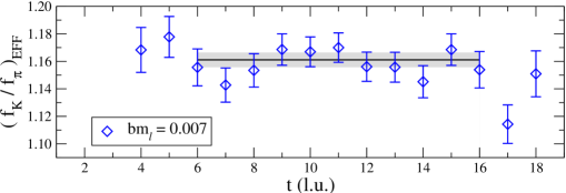
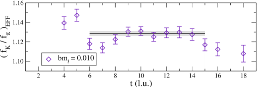
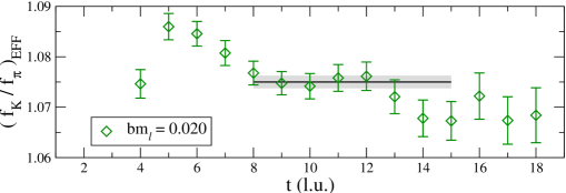
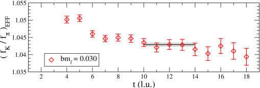
Figure 1: “Effective” $f_{K}/f_{\pi}$ determined from the smeared-smeared and smeared-point correlation functions with eq. (2). The solid black lines and shaded regions are the fits (with $1\sigma$ errors) tabulated in Table 2.

In order to extract the amplitudes for the smeared-smeared and smeared-point correlation functions a single exponential with a common mass was fit by $\chi^{2}$-minimization to each data set, i.e. a three parameter fit was performed with variables ${\cal A}_{P}^{ss}$, ${\cal A}_{P}^{sp}$ and $m_{\pi}$ (or $m_{K}$). The central value and uncertainty of each parameter was determined by the jackknife procedure over the ensemble of configurations. The decay constant was extracted by jackknifing over the appropriate combination of quantities, as given in eq. (1). In fig. 1 we present the lattice data using “effective” $f_{K}/f_{\pi}$ plots according to eq. (2), along with the fits.

Table 2: Calculated quantities with fitting ranges in brackets. All errors are computed using the jackknife procedure. Values for ${\cal F}$ are given without and with (in squiggly brackets) the $log^{2}$ contribution.

Ensemble	$m_{\pi}$(GeV)	$m_{\pi}/f_{\pi}$	$m_{K}/f_{\pi}$	$f_{K}/f_{\pi}$	${\cal F}\times 10^{3}$
m007	0.2931(15)	1.978(19) [5-16]	3.937(28) [6-16]	1.1610(54) [6-16]	5.67(6) {5.31(5)}
m010	0.3546(9)	2.337(11) [5-16]	3.958(16) [6-15]	1.1286(23) [6-15]	5.62(3) {5.13(2)}
m020	0.4934(12)	3.059(12) [7-16]	3.988(15) [7-15]	1.0751(13) [8-15]	5.68(3) {4.87(2)}
m030	0.5918(10)	3.484(10) [5-15]	4.004(12) [7-14]	1.04279(69) [10-14]	5.73(2) {4.69(2)}

The results of the lattice calculation of the decay constants and meson masses are tabulated in Table 2.

III.1 Chiral Extrapolation at Next-to-Leading Order

In $SU(3)$ chiral perturbation theory ($\chi$PT) Gasser and Leutwyler Gasser and Leutwyler (1985, 1984, 1983) showed that the ratio of the kaon to pion decay constants is given, at next-to-leading order (NLO) in the chiral expansion, by

$$\frac{f_{K}}{f_{\pi}}=1+\frac{5}{4}l_{\pi}(\mu)-\frac{1}{2}l_{K}(\mu)-\frac{3}{4}l_{\eta}(\mu)+\frac{8}{f^{2}}\left(m^{2}_{K}-m^{2}_{\pi}\right)L_{5}(\mu)$$ (4)

where $f$ is the pseudoscalar decay constant in the chiral limit, $m_{K}$ is the kaon mass, $m_{\pi}$ is the pion mass, and

$$l_{i}(\mu)\equiv\frac{1}{16\pi^{2}}\frac{m_{i}^{2}}{f^{2}}\log\left(\frac{m_{i}^{2}}{\mu^{2}}\right),$$ (5)

with the index $i$ running over the pseudoscalar states ($\pi$,$K$ and $\eta$). $L_{5}(\mu)$ is a Gasser-Leutwyler low-energy constant evaluated at the $\chi$PT renormalization scale $\mu$, whose scale dependence exactly compensates the scale dependence of the logarithmic contributions.

In our lattice calculation we have not computed the mass of the $\eta$ meson since it involves disconnected diagrams that require significant computer time to evaluate. Hence we replace $m_{\eta}$ with its value obtained from the Gell-Mann-Okubo mass-relation among octet mesons,

$$m_{\eta}^{2}=\frac{4}{3}m_{K}^{2}-\frac{1}{3}m_{\pi}^{2}\ \ ,$$ (6)

which is valid to the order of $\chi$PT to which we are working. In addition, we choose to work with $\mu=f_{\pi}^{\it phy}$, the value of the pion decay constant at the physical point. To recover the value of the counterterm $L_{5}(\mu)$ at some other renormalization scale, one can use the evolution Gasser and Leutwyler (1985, 1984, 1983)

$$L_{5}(f_{\pi}^{\it phy})=L_{5}(\mu)-\frac{3}{8}\frac{1}{16\pi^{2}}\log\left(\frac{f_{\pi}^{\it phy}}{\mu}\right)\ .$$ (7)

Finally, we replace the ratios $(m_{i}/f_{\pi}^{\it phy})^{2}$ by the lattice-computed value $(m_{i}/f_{\pi})^{2}$, which is again consistent to the order of $\chi$PT to which we are working. Hence, the final NLO expression to which we fit the lattice data is

$$\frac{f_{K}}{f_{\pi}}=1 + \frac{5}{4}\frac{1}{16\pi^{2}}\frac{m_{\pi}^{2}}{f_{\pi}^{2}}\log\left(\frac{m_{\pi}^{2}}{f_{\pi}^{2}}\right)-\frac{1}{2}\frac{1}{16\pi^{2}}\frac{m_{K}^{2}}{f_{\pi}^{2}}\log\left(\frac{m_{K}^{2}}{f_{\pi}^{2}}\right)$$ (8)

$$- \frac{1}{16\pi^{2}}\left(\frac{m_{K}^{2}}{f_{\pi}^{2}}-\frac{1}{4}\frac{m_{\pi}^{2}}{f_{\pi}^{2}}\right)\log\left(\frac{4}{3}\frac{m_{K}^{2}}{f_{\pi}^{2}}-\frac{1}{3}\frac{m_{\pi}^{2}}{f_{\pi}^{2}}\right)+8\left(\frac{m_{K}^{2}}{f_{\pi}^{2}}-\frac{m_{\pi}^{2}}{f_{\pi}^{2}}\right)L_{5}(f_{\pi}^{\it phy})\ .$$

Note that the only parameter to be determined by fitting at NLO is $L_{5}$. It is also worth noting that the above expression has the expected behavior that at the $SU(3)$ symmetric point the ratio of decay constants is unity.

For reasons that will become clear below, it is useful to “linearize” the fitting procedure by isolating the analytic terms with coefficients that are to be fit to the lattice data. We define the function

$${\cal F}\equiv\left(\frac{f_{K}}{f_{\pi}}-1-\chi_{logs}\right)\frac{1}{8\ y}\ ,$$ (9)

where, at NLO,

$$\chi_{logs}\ =\ \chi_{logs}^{(NLO)}\left(\frac{m_{\pi}}{f_{\pi}},\frac{m_{K}}{f_{\pi}}\right)= \frac{5}{4}\frac{1}{16\pi^{2}}\frac{m_{\pi}^{2}}{f_{\pi}^{2}}\log\left(\frac{m_{\pi}^{2}}{f_{\pi}^{2}}\right)-\frac{1}{2}\frac{1}{16\pi^{2}}\frac{m_{K}^{2}}{f_{\pi}^{2}}\log\left(\frac{m_{K}^{2}}{f_{\pi}^{2}}\right)$$ (10)

$$-\frac{1}{16\pi^{2}}\left(\frac{m_{K}^{2}}{f_{\pi}^{2}}-\frac{1}{4}\frac{m_{\pi}^{2}}{f_{\pi}^{2}}\right)\log\left(\frac{4}{3}\frac{m_{K}^{2}}{f_{\pi}^{2}}-\frac{1}{3}\frac{m_{\pi}^{2}}{f_{\pi}^{2}}\right)\ \ \ ,$$

and the quantity $y$ is

$$y=\frac{m^{2}_{K}}{f_{\pi}^{2}}-\frac{m^{2}_{\pi}}{f_{\pi}^{2}}\ .$$ (11)

Therefore, at NLO in the chiral expansion, the quantity ${\cal F}$ should be the same on each of the ensembles, and equal to the counterterm $L_{5}(f_{\pi}^{\it phy})$,

$${\cal F} = L_{5}(f_{\pi}^{\it phy})\ \ \ .$$ (12)

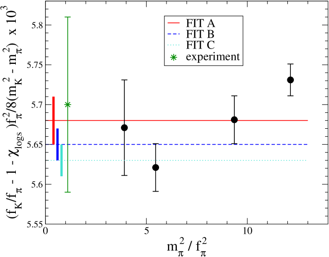
Figure 2: ${\cal F}$ vs. $m^{2}_{\pi}/f^{2}_{\pi}$ at NLO, along with the three different fits, A, B and C. The solid bars near the y-axis denote the value of $L_{5}$ and its uncertainty from the three fits. The point denoted by the star corresponds to the experimental value.

The calculated values of ${\cal F}$, along with their uncertainties determined by jackknifing over the configurations, are shown in Table 2, and in fig. 2 we have plotted ${\cal F}$ versus $m_{\pi}^{2}/f_{\pi}^{2}$. A $\chi^{2}$-minimization is performed to extract the one parameter $L_{5}(f_{\pi}^{\it phy})$ from the data. It is clear that the data is not that well fit by a constant, due to the presence of higher-order terms in the chiral expansion, and so to explore the dependence on these higher order terms we have sequentially “pruned” the data by removing the highest mass point ($bm_{l}=030$), and then the two highest mass points ($bm_{l}=030$, $020$) and determined $L_{5}(f_{\pi}^{\it phy})$ . The results of these fits are shown in fig. 2, and presented in Table 3.

Table 3: Results from chiral extrapolation at one-loop order in $\chi$PT. Explanation of the various fits is in the text.

FIT	$L_{5}\times 10^{3}$	$f_{K}/f_{\pi}$ (extrapolated)	$\chi^{2}$/dof
A	$5.68(3)$	$1.221(3)$	$3.5$
B	$5.65(2)$	$1.218(2)$	$1.4$
C	$5.63(2)$	$1.215(2)$	$0.7$

With the value of $L_{5}$, we use eq. 8 to evaluate the ratio of the decay constants at the physical point using the physical values for the pseudoscalar masses and the pion decay constant Eidelman et al. (2004),

$$f_{\pi^{+}} = 130.7~{}{\rm MeV}\ ,\ m_{\pi}\ =\ 137.3~{}{\rm MeV}\ ,\ m_{K}\ =\ 495.7~{}{\rm MeV},$$ (13)

where the masses are the isospin-averaged values. We use the Gell-Mann–Okubo mass relation to determine the $\eta$-mass that appears in the chiral contributions.

It is important to keep in mind that this determination of $L_{5}$ is only perturbatively close to the actual value of $L_{5}$ which is defined in the chiral limit. In the current extraction, the strange quark mass is held fixed near the physical value, while the light quark masses are somewhat lighter.

III.2 Incomplete Chiral Extrapolations at Next-to-Next-to-Leading Order

While the full two-loop expressions for ${f_{K}}/{f_{\pi}}$ exist in both QCD Amoros et al. (2000) and partially-quenched QCD Bijnens et al. (2006), these expressions contain many fit parameters, and therefore fruitful use of these results must await lattice data with better statistics and at a larger variety of quark masses. In order to estimate systematic errors, we perform fits with parts of the next-to-next-to-Leading-Order (NNLO) expression Bijnens et al. (1998). We focus on just two of the structures that enter at NNLO, analytic terms and a double logarithm with fixed coefficient.

III.2.1 Partial $N^{2}LO$ : Analytic Terms Only

Including only the analytic terms that enter at NNLO, eq. (12) becomes

$${\cal F} = L_{5}\ +\ C_{s}\ m_{s}\ +\ C_{l}\ m_{l}$$ (14)

$$= \tilde{L}_{5}\ +\ \tilde{C}_{\pi}\ \frac{m_{\pi}^{2}}{f_{\pi}^{2}}\ \ \ ,$$

where terms higher order in the chiral expansion are not shown. As the strange quark mass is the same over all ensembles, we simply absorb it into the definition of $L_{5}$, making explicit the quark mass dependence discussed previously. Therefore fitting at NNLO holding the strange quark mass fixed introduces one additional fit parameter, $\tilde{C}_{\pi}$. It is clear that the values of $\tilde{L}_{5}$ and $\tilde{C}_{\pi}$ extracted from the data are correlated, and in determining the extrapolated value of $f_{K}/f_{\pi}$ we explore the entire 68% confidence-level error ellipse in the $\tilde{L}_{5}-\tilde{C}_{\pi}$ plane  (shown in fig. 4). We label this fit D, and the results are shown in Table 4.

Table 4: Results from fitting the partial NNLO chiral contributions. Explanation of fits D,E,F and G are in the text.

FIT	${\tilde{L}}_{5}\times 10^{3}$	$\tilde{C}_{\pi}\times 10^{5}$	$f_{K}/f_{\pi}$ (extrapolated)	$\chi^{2}$/dof
D	$5.55(5)$	$\;\;1.40(49)$	$1.209(8)$	$0.8$
E	$5.53(4)$	$-7.00(47)$	$1.209(7)$	$1.0$
F	$5.80(3)$	$-8.28(35)$	$1.224(5)$	$0.5$
G	$5.16(5)$	$-4.93(56)$	$1.205(9)$	$1.5$

The data minus the NLO chiral logs, and the fit are shown in fig. 3.

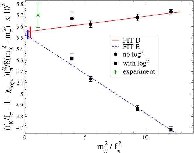
Figure 3: ${\cal F}$ vs. $m^{2}_{\pi}/f^{2}_{\pi}$ at NNLO. The solid bars near the y-axis denote the value of $\tilde{L}_{5}={\cal F}(m_{\pi}=0)$ and its uncertainty from the fits. The point denoted by the star corresponds to the experimental value. The circles denote the lattice data with only the NLO chiral logs subtracted, while the squares are the lattice data with the NLO chiral logs and the NNLO $\log^{2}$ term subtracted.

Note that the errors quoted in Table 4 and displayed in fig. 3 are $1\sigma$ errors.

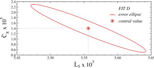
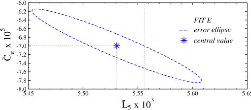
Figure 4: 68% confidence-level error ellipses for fits D and E described in the text.

III.2.2 Partial $N^{2}LO$ : Analytic Terms and Double Chiral Logs

The full two-loop expression that contributes to $f_{K}/f_{\pi}$ is quite complicated. An approximation to the $\log^{2}$ piece at two-loop order can be evaluated using renormalization-group techniques and is given by Bijnens et al. (1998)

$$\chi_{\log^{2}}^{(NNLO)} = \frac{1}{6144\pi^{4}}\left(\frac{m^{2}_{K}}{f_{\pi}^{2}}-\frac{m^{2}_{\pi}}{f_{\pi}^{2}}\right)\left(17\frac{m^{2}_{K}}{f_{\pi}^{2}}+37\frac{m^{2}_{\pi}}{f_{\pi}^{2}}\right)\log\left(\frac{M^{2}}{\mu^{2}}\right)^{2}\ \ ,$$ (15)

where $M$ is a mass scale related to the Goldstone boson masses. It would seem reasonable to choose the intermediate mass scale $M=\sqrt{m_{\pi}m_{K}}$ and $\mu=f_{\pi}$. Of course, the two-loop contributions vanish at the flavor $SU(3)$ symmetric point. Again, to isolate the fitting function, we subtract $\chi_{\log^{2}}^{(NNLO)}$ from the lattice data, giving a fit function of the form

$${\cal F}\equiv\left(\frac{f_{K}}{f_{\pi}}-1-\chi_{logs}^{(NLO)}-\chi_{\log^{2}}^{(NNLO)}\right)\frac{1}{8\ y}\ =\ \tilde{L}_{5}(f_{\pi}^{\it phy})\ +\ \tilde{C}_{\pi}\ \frac{m_{\pi}^{2}}{f_{\pi}^{2}}\ .$$ (16)

The scale dependence of the $\log^{2}$ contribution requires that the coefficients $C_{s}$ and $C_{u}$ in eq. (14) be scale-dependent, and thus $\tilde{C}_{\pi}$ becomes scale-dependent and the scale-dependence of $\tilde{L}_{5}$ is modified (a higher order effect). The calculated values of ${\cal F}$, along with their uncertainties determined by jackknifing over the configurations, are shown in Table 2, and plotted in fig. 3. We anticipate that the fit value of $\tilde{L}_{5}$ should change only a small amount from its value obtained in the NLO fits and in fit D, if the chiral expansion is convergent. However, we expect that the coefficient $\tilde{C}_{\pi}$ could change by an amount of order one. The results of fitting this functional form to the lattice data, which we denote by fit E, are presented in Table 4, and shown in fig. 3 (error ellipse is shown in fig. 4). Indeed, $\tilde{L}_{5}$ is changed very little, while $\tilde{C}_{\pi}$ changes by an amount of order one. We also give results for fits F and G which are the same as fit E except the argument of the $log^{2}$ contribution is chosen to be $M=m_{\pi}$ and $M=m_{K}$, respectively. These choices lead to a larger variation in $\tilde{L}_{5}$ and consequently in $f_{K}/f_{\pi}$.

III.3 Discussion

To determine $f_{K}/f_{\pi}$ at the physical point and its associated uncertainty we synthesize the results of the NLO and NNLO fits. Fitting the lowest two mass points at NLO gives $f_{K}/f_{\pi}=1.215\pm 0.002$, while fitting the three data points with pion masses below $m_{\pi}\sim 500~{}{\rm MeV}$ gives $f_{K}/f_{\pi}=1.218\pm 0.002$. The difference between them is within statistical errors ($1.5\sigma$) but there appears to be a systematic trend in the data which can be attributed to higher orders in the chiral expansion. As we are unable to fit the full NNLO expression to our small data set we can estimate the systematic uncertainty in this calculation by looking at the range of values of $f_{K}/f_{\pi}$ that result from the two types of NNLO extrapolation, both with and without the $\log^{2}$ contribution, including variation in the argument of the NNLO logarithm and including statistical errors. The range of variation in the NNLO estimate is an order of magnitude larger than the statistical error found at NLO. We take this NNLO uncertainty, $\Delta(f_{K}/f_{\pi})=^{+0.011}_{-0.022}$, to be an estimate of the systematic error in our calculation due to the truncation of the chiral expansion. We also assign a systematic error due to fitting procedures, obtained by varying the fitting ranges displayed in fig. 1, which gives $\Delta(f_{K}/f_{\pi})=^{+0.000}_{-0.010}$. Therefore, our final number is:

$$\frac{f_{K}}{f_{\pi}}=1.218\pm 0.002\ ^{+0.011}_{-0.024}\ ,$$ (17)

where the first error is statistical and the second error is systematic, with the extrapolation error and fitting error added in quadrature. The error in this lattice QCD determination of ${f_{K}}/{f_{\pi}}$ is clearly dominated by the systematics.

Using a similar procedure, we arrive at a value for $L_{5}$:

$$L_{5}(f_{\pi}^{\it phy}) = 5.65\pm 0.02\ ^{+0.18}_{-0.54}\ \times\ 10^{-3}\ \ ,$$ (18)

where the first error is statistical and the second is an estimate of the systematic error due to omitted higher orders in the chiral expansion. This then scales to give $L_{5}(m_{\eta}^{\it phy})=2.22\pm 0.02\ ^{+0.18}_{-0.54}\,\times\,10^{-3}$ at the $\eta$-mass and $L_{5}(m_{\rho}^{\it phy})=1.42\pm 0.02\ ^{+0.18}_{-0.54}\,\times\,10^{-3}$ at the $\rho$-mass. As stated previously, this is an effective $L_{5}$ as it includes the higher order strange quark contribution.

The results for $f_{K}/f_{\pi}$ have an additional systematic error due to the non-zero lattice spacing which we expect to be $O((m_{s}-m_{u})b^{2})$. In principle one can reduce this error by fitting to the appropriate $\chi$PT formulas that include the $O(g^{2}b^{2})$ effects due to flavor-symmetry breaking in the sea-quark sector Bar et al. (2005). However, our data fit well to the continuum $\chi$PT formulas and hence we do not expect that use of the extended $\chi$PT formulas of Ref. Bar et al. (2005) would significantly improve our results at this stage. Our final result is consistent with the MILC number Aubin et al. (2004)

$$\left.\frac{f_{K}}{f_{\pi}}\right|_{\rm MILC}=1.210\pm 0.004\pm 0.013\ ,$$ (19)

where the first error is statistical and the second is the total systematic error estimated by MILC. Since our valence quarks are domain-wall fermions, in contrast with the KS quarks used by MILC, the discretization errors should be different. Hence, the agreement of our results to the few-percent level is further confirmation that these systematic errors are small .

It is also interesting to note that our result is in agreement with the experimental number,

$$\left.\frac{f_{K}}{f_{\pi}}\right|_{\rm EXP}=1.223\pm 0.012\ \ ,$$ (20)

but our calculation has a somewhat larger systematic error due to uncertainty in the chiral extrapolation.

It is possible to further improve the precision of our calculation by increasing the statistics of the lighter pion masses, including one more point at even lighter pion mass, and by better utilizing the power of partial-quenching; i.e. by computing with different valence quark masses, away from the tuned point. We hope that with these improvements in place we will be able to improve upon the MILC result.

IV Conclusions

Existing high-precision calculations of basic standard model quantities involve staggered valence quarks on staggered sea quarks with their associated systematic errors. Clearly, it is important to employ a variety of fermion discretizations in order to understand and reduce one of the inherent systematic errors in lattice QCD calculations. We have computed $f_{K}/f_{\pi}$ with domain-wall valence quarks on MILC lattices and find results consistent with an earlier calculation by MILC using KS valence quarks. It is gratifying to find that using different fermions in the valence sector leads to a consistent precision determination of $f_{K}/f_{\pi}$ in accord with basic effective field theory expectations about the scaling of discretization errors.