$Id:sewm.tex,v1.32006/06/2307:38:00pbialasExppbialas$ SU(3) gauge theory at finite temperature in 2 + 1 dimensions B. Petersson

SU(3) gauge theory at finite temperature in 2 + 1 dimensions

Abstract

In this article we will discuss numerical results on screening masses and thermodynamic quantities in 2 + 1 dimensional SU(3) gauge theory. We will also compare them to perturbation theory and the dimensionally reduced model.

The SU(3) gauge theory in 2+1 dimensions is simple enough from a numerical point of view, so that it is possible with present computers to make continuum extrapolations with controlled systematic errors. Of course, there are some obvious differences between SU(3) gauge theory in 2 + 1 and 3 + 1 dimensions. In 2 + 1 dimensions the coupling constant $g^{2}$ has the dimension of a mass, and the theory is superrenormalizable. The tree level potential between heavy quarks is already logarithmically confining: $V(r)\sim\log r$. There are, however, many similarities. One may introduce a dimensionless “running” coupling constant $g_{3}(l)$ by the definition $g^{2}_{3}(l)\equiv lg^{2}$ where $l$ is a length scale. Then $g^{2}_{3}(l)\rightarrow 0$ for $l\rightarrow 0$ and to infinity for $l\rightarrow\infty$. This is somewhat analogous to the logarithmically running coupling constant in 3 + 1 dimensional SU(3) gauge theory. In 2 + 1 dimensions the coupling constant $g^{2}$ sets the scale, and $m_{i}=c_{i}g^{2}$, where $c_{i}$’s are numerical constants. From Monte Carlo simulations one knows some further properties: There is a linearly rising non-perturbative potential $V(r)\simeq\sigma_{0}r$ for $r$ large[1, 2]. There is a second order phase transition at $T_{c}=0.55(1)g^{2}$ , with the critical indices of the 2d 3states Potts model[2]. Furthermore, the glue ball masses $m_{GB}$ are much bigger than $T_{c},\,m_{GB}\geq 4.4T_{c}$ [1]. This is all qualitatively similar to 3 + 1 dimensions, where, however, the transition is weakly first order. In the gluon plasma phase $T>T_{c}$, one should be able to use perturbation theory. The relevant dimensionless coupling in 2 + 1 dimensions is

$$g^{2}_{3}(T)\equiv\frac{g^{2}}{T}\mathop{\longrightarrow}\limits^{T\rightarrow\infty}0.$$ (1)

There are, however, infrared divergences, which are even more serious than in 3 + 1 dimensions. For the screening mass (rsp. the pressure) they appear already at order $g^{2}$, i.e. at one (resp. two) loop(s). The infrared divergences can be tamed through resummations, e.g. through the selfconsistent perturbation theory (SCPT) introduced by D’Hoker[3]. It works in the following way. Choose the class of static gauges $\partial_{0}A_{0}(x)=0$ where the Polyakov loop is purely static,

$$L(\bar{x})=Tr\,e^{i\frac{g}{T}A_{0}(\bar{x})}.$$ (2)

Add and subtract an explicit mass term in the static sector,

$$\frac{1}{2}m^{2}_{g}\,Tr(A_{0}(\bar{x}))^{2},$$ (3)

which is invariant inside this class of gauges, and perform the perturbative expansion in the theory with $A_{0}$ massive. In fact, there are no further infrared divergencies in 2+1 dimensions[3].

The second method, which is semianalytic, is the dimensional reduction from 2 + 1 to 2 dimensions[4]. Again we choose the class of static gauges. We then integrate perturbatively over the non-static modes. This integration is by construction infrared finite. The result is an effective 2-dimensional adjoint Higgs model for the static modes with the action

$$S= \int\,d^{2}xTr\left\{\frac{1}{2}F_{ij}^{2}+(D_{i}\phi)^{2}-\frac{3g^{2}T}{2\pi}\left[\frac{5}{2}\log 2+1-\log(aT)\right]\phi^{2}+\frac{g^{4}}{32\pi}\phi^{4}\right\}$$ (4)

where $D_{i}$ is a covariant derivative and where the coupling constants are derived from a one loop integration over the static modes. This action is systematic in $\frac{g^{2}}{T}$, e.g. the term $\phi^{6}$ is multiplied by a constant proportional to $\frac{g^{6}}{T}$, and is neglected at high $T$.

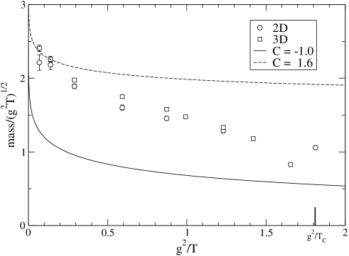
Figure 1: Screening masses from the 3D SU(3) theory on lattices with temporal extent $N_{\tau}=4$ compared to the predictions of SCPT(continuous lines) and to the 2D reduced model.

The two-dimensional adjoint Higgs model has not been solved analytically. We solve it non-perturbatively by a Monte Carlo lattice simulation.

We define a screening mass for $T>T_{c}$ by

$$\langle Re\left(L(0)L^{\dagger}(\vec{x})\right)\rangle\simeq\langle L\rangle^{2}+\frac{A}{\sqrt{m|\vec{x}|}}e^{-m|\vec{x}|}$$ (5)

In lowest order perturbation theory $m=2m_{g}$ for the correlations of $ReL(\bar{x})$ and $m=3m_{g}$ for the correlations of $Im\,L(\bar{x})$. In SCPT one has[3]

$$\frac{m^{2}_{g}}{g^{2}T}=\frac{3}{2\pi}\left(\log\frac{T}{m_{g}}+C\right)+{\cal O}\left(1/\log\frac{T}{m_{g}}\right),\quad C=-1.0.$$ (6)

In Fig. 1, we show $2m_{g}$ compared to the screening mass in the 2 + 1 dimensional SU(3) gauge theory. We have used the formula $T/T_{c}=(\beta-1.5)/3.3N_{\tau}$, derived from the condition $T_{c}/g^{2}=0.55$ for all $N_{\tau}$, and the values $\beta_{c}(N_{\tau})$ from[2]. Solving Eq. (6) where $m_{g}/T$ has been replaced by $(1-\exp(-m_{g}/T))$, we can get agreement only for $T/g^{2}>6$ ($T/T_{c}>12$), and this only by arbitrarily choosing $C=1.6$.

The dimensionally reduced model is in good agreement with the full theory already for $T>1.5T_{c}$ as can be seen in Fig. 1. A further investigation showed that the two exchanged states in the reduced model are simple poles, not 2 gluon and 3 gluon cuts respectively[5].

For the thermodynamics we use the lattice integral method introduced in [6].

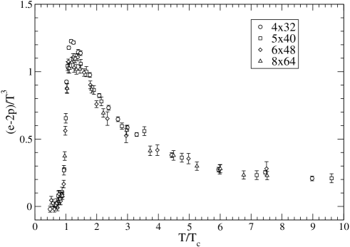
Figure 2: Trace anomaly $(\epsilon-2p)/T^{3}$, on lattices of various sizes.

The trace anomaly, $(\epsilon-2p)/T^{3}$, is presented in Fig. 2. It is qualitatively similar to the result in 3 + 1 dimensions.

Since the trace anomaly is zero for free massless gluons, we expect in perturbation theory that

$$\frac{\epsilon-2p}{T^{3}}\simeq\frac{g^{2}}{T}f\left(\log\frac{T}{g^{2}}\right).$$ (7)

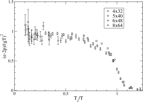
Figure 3: Check of the scaling formula (7).

In Fig. 3 we present $(\epsilon-2p)/T^{2}g^{2}$ as a function of $T_{c}/T$. One observes that this quantity is slowly varying at high temperature. A comparison with perturbation theory and dimensional reduction is in progress.

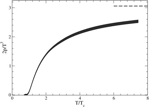
Figure 4: The pressure extrapolated to the infinite $N_{\tau}$ limit from the lattices of size $4\times 32^{2}$, $6\times 48^{2}$ and $8\times 64^{2}$ using a linear fit in $1/N^{2}_{\tau}$. The dashed line shows the Stefan-Boltzman limit.

In Fig. 4, we present the extrapolation of the pressure to the continuum.

This work is supported through ENRAGE (European Network on Random Geometry), a Marie Curie Research Training Network supported by the European Community’s Sixth Framework Programme, network contract MRTN-CT-2004-005616.

References

- [1] M. Teper, Phys. Rev D59 (1999) 014512.
- [2] C. Legeland, Thesis (Bielefeld 1998), J. Engels et al., Nucl. Phys. Proc. Suppl. 53 (1997) 430.
- [3] E. D’Hoker, Nucl. Phys. B201 (1982) 401.
- [4] P. Bialas et al., Nucl. Phys. B581 (2000) 471.
- [5] P. Bialas et al., Nucl. Phys. B603 (2001) 369.
- [6] J. Engels et al., Phys. Lett. B253 (1990) 625.