Moments of pseudoscalar meson distribution amplitudes from the lattice

Abstract

Based on lattice simulations with two flavours of dynamical, ${\cal O}(a)$-improved Wilson fermions we present results for the first two moments of the distribution amplitudes of pseudoscalar mesons at several values of the valence quark masses. By extrapolating our results to the physical masses of up/down and strange quarks, we find the first two moments of the $K^{+}$ distribution amplitude and the second moment of the $\pi^{+}$ distribution amplitude. We use nonperturbatively determined renormalisation coefficients to obtain results in the $\overline{\rm MS}$ scheme. At a scale of 4 GeV² we find $a_{2}^{\pi}=0.201(114)$ for the second Gegenbauer moment of the pion’s distribution amplitude, while for the kaon, $a_{1}^{K}=0.0453(9)(29)$ and $a_{2}^{K}=0.175(18)(47)$.

I Introduction

In recent years exclusive reactions with identified hadrons in the final and/or initial state are attracting increasing attention Brodsky and Lepage (1989). The reason for this interest is due to the fact that they are dominated by rare configurations of the hadrons’ constituents: either only valence-quark configurations contribute and all quarks have small transverse separation (hard mechanism) Chernyak and Zhitnitsky (1977, 1980); Efremov and Radyushkin (1980a, b); Lepage and Brodsky (1979, 1980); Chernyak et al. (1977, 1980), or one of the partons carries most of the hadron momentum (soft or Feynman mechanism). In both cases, the information about hadron structure is new and complementary to that in usual inclusive reactions, the prominent example being the deep-inelastic lepton hadron scattering.

Hard contributions are simpler to treat than their soft counterparts and their structure is well understood, see e.g. Ref. Stefanis et al. (2000) for a recent discussion. They can be calculated in terms of the hadron distribution amplitudes (DAs) which describe the momentum-fraction distribution of partons at zero transverse separation in a particular Fock state, with a fixed number of constituents. DAs are ordered by increasing twist; the leading twist-2 meson DA, $\phi_{\Pi}$, which describes the momentum distribution of the valence quarks in the meson $\Pi$, is related to the meson’s Bethe–Salpeter wave function $\phi_{\Pi,BS}$ by an integral over transverse momenta:

$$\phi_{\Pi}(x,\mu^{2})=Z_{2}(\mu^{2})\int^{|k_{\perp}|<\mu}\!\!d^{2}k_{\perp}\,\phi_{\Pi,BS}(x,k_{\perp}).$$

Here $x$ is the quark momentum fraction, $Z_{2}$ is the renormalisation factor (in the light-cone gauge) for the quark-field operators in the wave function, and $\mu$ denotes the renormalisation scale. In particular the leading-twist DA of the pion and of the nucleon have attracted much attention in the literature. Furthermore, $SU(3)$ flavour symmetry breaking effects in the DAs of strange mesons are important for predictions of the exclusive B-decay rates (e.g. $B\to K,K^{*}$) in the framework of QCD factorisation Beneke et al. (2000), perturbative QCD Keum and Li (2001), soft-collinear effective theory (SCET) Bauer et al. (2001, 2002) or light-cone sum rules, e.g. Ball and Braun (1998); Khodjamirian et al. (2000); Ball and Zwicky (2005a). In some cases, for instance weak radiative decays, $B\to\rho\gamma$ vs. $B\to K^{*}\gamma$, the uncertainty in $SU(3)$ breaking is actually the dominant source of theoretical error.

The theoretical description of DAs is based on their representation Chernyak and Zhitnitsky (1977, 1980); Efremov and Radyushkin (1980a, b); Lepage and Brodsky (1979, 1980); Chernyak et al. (1977, 1980) as matrix elements of a suitable nonlocal light-cone operator. For example, for positively charged pions or kaons one defines

$$\langle 0|\bar{q}(-z)\gamma_{\mu}\gamma_{5}[-z,z]u(z)|\Pi^{+}(p)\rangle=if_{\Pi}p_{\mu}\int_{-1}^{1}d\xi\,e^{-i\xi p\cdot z}\phi_{\Pi}(\xi,\mu^{2})\,,$$ (1)

where $q=d,s$, $z_{\mu}$ is a light-like vector, $z^{2}=0$, $[-z,z]$ is the straight-line-ordered Wilson line connecting the quark and the antiquark fields and $f_{\Pi}$ is the usual decay constant $f_{\pi}=132$ MeV, $f_{K}=160$ MeV Eidelman et al. (2004). The physical interpretation of the variable $\xi$ is that $x=(1+\xi)/2$ and $1-x=(1-\xi)/2$ are the fractions of the meson momentum carried by the quark and antiquark, respectively. The definition in (1) implies the normalisation

$$\int_{-1}^{1}d\xi\,\phi_{\Pi}(\xi,\mu^{2})=1\,.$$ (2)

For brevity, below we often drop the subscript and write $\phi$ instead of $\phi_{\Pi}$ unless we are referring to a specific meson.

A convenient tool to study DAs is provided by the conformal expansion Brodsky et al. (1980); Ohrndorf (1982); Braun et al. (2003); Makeenko (1981). The underlying idea is similar to the partial-wave decomposition in quantum mechanics and allows one to separate transverse and longitudinal variables in the Bethe–Salpeter wave–function. The dependence on transverse coordinates is formulated as a scale dependence of the relevant operators and is governed by renormalisation-group equations. The dependence on the longitudinal momentum fractions is described in terms of Gegenbauer polynomials $C^{3/2}_{n}(\xi)$ which are nothing but irreducible representations of the corresponding symmetry group, the collinear conformal group SL(2,$\mathbb{R}$).

In this way one obtains Makeenko (1981); Brodsky et al. (1980); Ohrndorf (1982); Efremov and Radyushkin (1980a, b); Lepage and Brodsky (1979, 1980)

$$\phi_{\Pi}(\xi,\mu^{2})=\frac{3}{4}(1-\xi^{2})\left(1+\sum\limits_{n=1}^{\infty}a^{\Pi}_{n}(\mu^{2})C_{n}^{3/2}(\xi)\right).$$ (3)

To leading-logarithmic accuracy (LO), the (non-perturbative) Gegenbauer moments $a_{n}$ renormalise multiplicatively with

$$a_{n}(\mu^{2})=L^{\gamma^{(0)}_{n}/(2\beta_{0})}\,a_{n}(\mu_{0}^{2}),$$ (4)

where $L\equiv\alpha_{s}(\mu^{2})/\alpha_{s}(\mu_{0}^{2})$, $\beta_{0}=11-2N_{f}/3$, and the anomalous dimensions $\gamma^{(0)}_{n}$ are given by

$$\gamma^{(0)}_{n}=8C_{F}\left(\sum_{k=1}^{n+1}\frac{1}{k}-\frac{3}{4}-\frac{1}{2(n+1)(n+2)}\right)$$ (5)

with $C_{F}=4/3$. Note that the multiplicative renormalisability in leading order is not an accident: It relies on the fact that the tree-level counterterms retain the symmetry properties of the Lagrangian Braun et al. (2003).

Since the anomalous dimensions increase with spin, the higher-order contributions in the Gegenbauer expansion are suppressed at large scales so that asymptotically only the leading term survives

$$\phi(\xi,\mu^{2}\to\infty)=\phi_{as}(\xi)=\frac{3}{4}(1-\xi^{2}).$$ (6)

For this reason, one usually assumes that the conformal expansion is well convergent at all scales of practical interest, and retaining the first few terms only in the conformal expansion provides one with a reasonable approximation for convolution integrals of the type $\int_{-1}^{1}d\xi\,\phi(\xi)/(1-\xi)$ that one encounters in many applications.

To next-to-leading order (NLO) accuracy, the scale dependence of the Gegenbauer moments is more complicated and reads Mikhailov and Radyushkin (1985); Mueller (1994, 1995)

$$a_{n}(\mu^{2})=a_{n}(\mu_{0}^{2})E_{n}^{\rm NLO}+\frac{\alpha_{s}(\mu^{2})}{4\pi}\sum_{k=0}^{n-2}a_{k}(\mu_{0}^{2})\,E_{k}^{\rm NLO}\,d^{(1)}_{nk}\,.$$ (7)

Here we adopt the usual convention that an empty sum is equal to zero. Moreover, $a_{0}=1$ and

$$E_{n}^{\rm NLO}=L^{\gamma^{(0)}_{n}/(2\beta_{0})}\left[1+\frac{\gamma^{(1)}_{n}\beta_{0}-\gamma_{n}^{(0)}\beta_{1}}{8\pi\beta_{0}^{2}}\Big{[}\alpha_{s}(\mu^{2})-\alpha_{s}(\mu_{0}^{2})\Big{]}\right]\,,$$ (8)

where $\gamma^{(1)}_{n}$ are the diagonal two-loop anomalous dimensions Mertig and van Neerven (1996), $\beta_{1}=102-(38/3)N_{f}$, and the mixing coefficients $d^{(1)}_{nk}$, $k\leq n-2$, are given in closed form in Ref. Mueller (1994, 1995), see also, for instance, Ref. Bakulev et al. (2004) for a recent compilation. For the lowest moments $n=0,1,2$ one needs

$$\gamma_{0}^{(1)}=0\,,\qquad\gamma_{1}^{(1)}=\frac{23488}{243}-\frac{512}{81}\,N_{f}\,,\qquad\gamma_{2}^{(1)}=\frac{34450}{243}-\frac{830}{81}\,N_{f}$$ (9)

and

$$d^{(1)}_{20}=\frac{7}{30}(5C_{F}-\beta_{0})\frac{\gamma^{(0)}_{2}}{\gamma^{(0)}_{2}-2\beta_{0}}\left[1-L^{-1+\gamma^{(0)}_{2}/(2\beta_{0})}\right].$$ (10)

If the mass difference between the $u$ and $d$ quarks is neglected, $G$-parity implies that the pion DA $\phi_{\pi}(\xi,\mu)$ is an even function of $\xi$, i.e all odd moments in $\xi$, $a^{\pi}_{2n+1}$, vanish. The K-meson DA need not be even, and the calculation of $a^{K}_{1}$ will be one of our goals.

The coefficients $a_{n}$ at some reference scale $\mu_{0}$ are nonperturbative quantities and have to be evaluated using a nonperturbative technique or must be extracted from experiment. In historic perspective, most of the discussion over the years was centered on a particular model of the pion DA proposed by Chernyak and Zhitnitsky in 1982 on the basis of their calculation of $a_{2}^{\pi}$ using QCD sum rules Chernyak and Zhitnitsky (1982). Using this model and assuming dominance of the hard rescattering mechanism in exclusive reactions, Chernyak and Zhitnitsky were able to describe an impressive amount of experimental data that were available at that time Chernyak and Zhitnitsky (1984).

Since then, the original argumentation by Chernyak and Zhitnitsky and the model itself have been largely discredited. Three different approaches have been used: direct calculations using QCD sum rules, pioneered in Chernyak and Zhitnitsky (1982); analysis of experimental data on the pion electromagnetic and transition form factors (e.g. Stefanis et al. (1999)) and the $B$ weak decay form factor, using light-cone sum rules; and lattice calculations. The summary of these results is presented in Table 2 of Ref. Ball et al. (2006); see also, for instance, Refs. Bakulev et al. (2003, 2004) for another recent compilation. It turns out that $a_{2}^{\pi}$ can only be determined with large errors, whatever approach is chosen. A fair average is probably

$$a_{2}^{\pi}(4\,{\rm GeV}^{2})=0.17\pm 0.15\,.$$ (11)

The $K$-meson DA has attracted comparatively less attention. The numerical value of the first moment $a^{K}_{1}$ was the subject of significant controversy until recently. The existing estimates are all obtained using different versions of QCD sum rules Khodjamirian et al. (2004); Braun and Lenz (2004); Ball and Zwicky (2006a, b) and yield an average Ball et al. (2006)

$$a_{1}^{K}(4\,{\rm GeV}^{2})=0.05\pm 0.03.$$ (12)

For the second moment, the old estimate by Chernyak and Zhitnitsky was $a_{2}^{K}/a_{2}^{\pi}=0.59\pm 0.04$. Two recent sum rule calculations Khodjamirian et al. (2004); Ball et al. (2006), including radiative corrections to the sum rules, give however $a_{2}^{K}/a_{2}^{\pi}\simeq 1$ pointing towards a very small $SU(3)$ violation in this coefficient.

Estimates of yet higher-order Gegenbauer coefficients are rather uncertain. The light-cone sum-rule calculations of the transition form factor $F_{\pi\gamma\gamma^{*}}$ in Refs. Schmedding and Yakovlev (2000); Bakulev et al. (2003, 2006); Agaev (2005) suggest a negative value for $a_{4}^{\pi}$, which is consistent with the result $a_{4}^{\pi}(1\,{\rm GeV}^{2})>-0.07$ obtained in Ref. Ball and Zwicky (2005b). However, this conclusion may be premature because yet higher moments have been omitted (however, in Ref. Bakulev et al. (2001) they are estimated to be small). Moreover, there does not seem to be any convincing method to estimate the uncertainty due to the model dependence of the analysis. While it seems that distribution amplitude moments beyond the second are extremely difficult to access on the lattice, it might be possible to estimate them using the transverse lattice approach Dalley and van de Sande (2003) or from the operator product expansion in lattice QCD Capitani et al. (1999); Detmold and Lin (2006).

Last but not least, we have to mention the estimate of the pion DA in the middle point where the momentum is shared equally between the quark and the antiquark Braun and Filyanov (1989)

$$\phi_{\pi}(\xi=0)=0.6\pm 0.15\ ,$$ (13)

and the measurement of the pion DA in diffractive dijet production by E791 Aitala et al. (2001). Unfortunately, it turns out that collinear factorisation is broken for dijet production Braun et al. (2001, 2002), so that the interpretation of this beautiful experiment is not straightforward, see also Chernyak (2001); Chernyak and Grozin (2001).

The lattice computation of DAs of pseudoscalar $\pi$ and $K$ mesons will be at the focus of this paper. On the lattice, we cannot compute non-local matrix elements of the form (1). However, via the light-cone operator product expansion (OPE), moments $\langle\xi^{n}\rangle$ of the DAs defined by

$$\langle\xi^{n}\rangle_{\Pi}(\mu^{2})=\int_{-1}^{1}d\xi\,\xi^{n}\phi_{\Pi}(\xi,\mu^{2})\ ,$$ (14)

are related to matrix elements of the local operators

$$\mathcal{O}^{M}_{\mu_{0}\ldots\mu_{n}}(0)=i^{n}\bar{q}(0)\gamma_{\mu_{0}}\gamma_{5}\stackrel{{\scriptstyle\leftrightarrow}}{{D}}_{\mu_{1}}\ldots\stackrel{{\scriptstyle\leftrightarrow}}{{D}}_{\mu_{n}}u(0)\ ,$$ (15)

by

$$\langle 0|\mathcal{O}^{M}_{\{\mu_{0}\ldots\mu_{n}\}}(0)|\Pi(p)\rangle=if_{\Pi}\,p_{\{\mu_{0}}\ldots p_{\mu_{n}\}}\,\langle\xi^{n}\rangle_{\Pi}\,.$$ (16)

Here $M$ refers to the fact that the operator is defined in Minkowski space, $D_{\mu}$ is the covariant derivative, $\stackrel{{\scriptstyle\leftrightarrow}}{{D}}=\stackrel{{\scriptstyle\rightarrow}}{{D}}\!-\!\stackrel{{\scriptstyle\leftarrow}}{{D}}$ and $\{\ldots\}$ denotes the symmetrisation of all indices and the subtraction of traces. The moments $\langle\xi^{n}\rangle$ are related to the Gegenbauer moments $a_{n}$ by simple algebraic relations:

$$a_{1}=\frac{5}{3}\langle\xi\rangle\,,\qquad a_{2}=\frac{7}{12}\left(5\langle\xi^{2}\rangle-1\right)\,,\qquad\mathrm{etc.}$$ (17)

Although the first lattice calculation of $\langle\xi^{2}\rangle_{\pi}$ appeared almost 20 years ago Kronfeld and Photiadis (1985); Martinelli and Sachrajda (1987), there has been surprisingly little activity in this area in recent times Daniel et al. (1991); Del Debbio et al. (2000, 2003) to complement other theoretical investigations. Our preliminary result for $\langle\xi^{2}\rangle_{\pi}$ was presented in Göckeler et al. (2005a) and we found in the $\overline{\rm MS}$ scheme at $\mu^{2}=5\,{\rm GeV}^{2}$, $\langle\xi^{2}\rangle_{\pi}^{\overline{\rm MS}}(\mu^{2}=5\,{\rm GeV}^{2})=0.281(28)$. This represents the most recent lattice result. The authors of Ref. Del Debbio et al. (2003), on the other hand, performed a simulation in quenched QCD and renormalised their results perturbatively to the $\overline{\rm MS}$ scheme at $\mu^{2}=7.1289$ GeV², $\langle\xi^{2}\rangle^{\overline{\rm MS}}_{\pi}(\mu^{2}=7.1289\,{\rm GeV}^{2})=0.280(49)^{+0.030}_{-0.013}\ .$

This paper is organised as follows. In Sec. II we describe our lattice technology including the operators and renormalisation prescriptions used. Section III contains our numerical results together with appropriate extrapolations towards the physical limits. Finally, in Sec. IV we summarise our findings by considering the results in terms of Gegenbauer moments. Here we also discuss the insights that we gain on the shape of the Pion and Kaon distribution amplitudes. We tabulate our results in Appendix A.

II Lattice techniques

We define a meson two-point correlation function in Euclidean space as

$$C^{\cal O}(t,\vec{p})=\sum_{\vec{x}}e^{-i\vec{p}\cdot\vec{x}}\left\langle{\cal O}_{\{\mu_{0}\dots\mu_{n}\}}(\vec{x},t)J(\vec{0},0)^{\dagger}\right\rangle\ ,$$ (18)

$$\rightarrow \frac{A}{2E}\langle 0|{\cal O}_{\{\mu_{0}\dots\mu_{n}\}}(0)|\Pi(p)\rangle\left[e^{-Et}+\tau_{\cal O}\tau_{J}e^{-E(L_{t}-t)}\right],\ \ 0\ll t\ll L_{t}\,,$$

where ${\cal O}_{\{\mu_{0}\dots\mu_{n}\}}$ is the Euclidean lattice transcription of Eq. (15),

$${\cal O}_{\{\mu_{0}\dots\mu_{n}\}}=\bar{q}\gamma_{\{\mu_{0}}\gamma_{5}\overset{\leftrightarrow}{D}_{\mu_{1}}\dots\overset{\leftrightarrow}{D}_{\mu_{n}\}}u\,,$$ (19)

$A=\langle\Pi(p)|J(0)^{\dagger}|0\rangle$, $E=\sqrt{m_{\Pi}^{2}+\vec{p}\,^{2}}$, $L_{t}$ is the temporal extent of the lattice and we use $J(x)\equiv\Pi(x)=\overline{q}(x)\gamma_{5}u(x)$ or $J(x)\equiv A_{4}(x)\equiv{\cal O}_{4}=\overline{q}(x)\gamma_{4}\gamma_{5}u(x)$ as the interpolating operator for the pseudoscalar mesons. The $\tau$ factor tells us how the operator behaves under time reversal, $t\to L_{t}-t$. We find that for $\tau_{J}$, $\tau_{\Pi}=-$ while $\tau_{A_{4}}=+$.

To increase the overlap of our interpolating operators with the ground state, we perform Jacobi smearing at the source Best et al. (1997), while the operators we use at the sink are local. Finally, we note that when working with operators involving derivatives, we perform the Fourier transform in Eq. (18) at the “centre-of-mass” of the operator Göckeler et al. (2006a).

II.1 Choice of operators

We need to choose the lattice operators to perform the matching of the appropriate representations of the H$(4)$ group — the group of Euclidean lattices relevant for our numerical computations — to the corresponding representations of the O$(4)$ group — the group of rotations and reflections in four Euclidean dimensions.

For the first moment of pseudoscalar mesons containing non-degenerate mass quarks we consider two types of operators which we denote generically by ${\cal O}^{a}_{\mu\nu}(\mu\neq\nu)$ and ${\cal O}^{b}_{\mu\mu}$, e.g.

$${\cal O}^{a}_{41}\!\! = \!\!{\cal O}_{\{41\}}\,,$$ (20)

$${\cal O}^{b}_{44}\!\! = \!\!{\cal O}_{\{44\}}-\frac{1}{3}\bigg{(}{\cal O}_{\{11\}}+{\cal O}_{\{22\}}+{\cal O}_{\{33\}}\bigg{)}\,.$$ (21)

The first operator, ${\cal O}^{a}_{41}$, requires a nonzero momentum component in the $1$-direction which we choose as small as possible, i.e., we take $\vec{p}=(p,0,0)$, where $p=2\pi/L_{s}$ and $L_{s}$ is the spatial extent of our lattice. Using rotational symmetry, we average over the momentum choices $\vec{p}=(0,p,0)$ and $\vec{p}=(0,0,p)$, using the operators in Eq. (20) with $\{41\}$ replaced with $\{42\}$ and $\{43\}$, respectively. The second operator, ${\cal O}^{b}_{\mu\mu}$, can be evaluated at $\vec{p}=(0,0,0)$.

In this situation, there will be no mixing with operators of equal or lower dimensions, however there are improvement terms that could be included Capitani et al. (2001). Unfortunately the improvement coefficients are not known, so we are forced to neglect their contribution, however they are expected to be small and as such are unlikely to affect our results.

For the case of the second moment, which appears for mesons with both degenerate and non-degenerate mass quarks, we also have two classes of operators ${\cal O}^{a}_{\mu\nu\rho}$, ${\cal O}^{b}_{\mu\nu\nu}$ Göckeler et al. (2005b), e.g.

$${\cal O}^{a}_{412} = {\cal O}_{\{412\}}\,,$$ (22)

$${\cal O}^{b}_{411} = {\cal O}_{\{411\}}-\frac{{\cal O}_{\{422\}}+{\cal O}_{\{433\}}}{2}\,.$$ (23)

From Eq. (16), we see that ${\cal O}^{a}_{\mu\nu\rho}$ requires two non-vanishing spatial components of momentum, $\vec{p}=(p,p,0)$, while ${\cal O}^{b}_{\mu\nu\nu}$ needs only one, $\vec{p}=(p,0,0)$. Consideration of this fact alone would lead one to choose ${\cal O}^{b}_{\mu\nu\nu}$, since momentum components in different directions on the lattice lead to a poorer signal. However, lattice operators with two or more covariant derivatives can mix with operators of the same or lower dimension. It turns out that for forward matrix elements, ${\cal O}^{b}_{\mu\nu\nu}$ suffers from such mixings while ${\cal O}^{a}_{\mu\nu\rho}$ does not.

For matrix elements involving a momentum transfer between the two states, i.e., nonforward matrix elements, both operators ${\cal O}^{a}_{\mu\nu\rho}$ and ${\cal O}^{b}_{\mu\nu\nu}$ can mix with operators involving external ordinary derivatives, i.e. operators of the form $\partial_{\mu}\partial_{\nu}\cdots(\bar{q}\cdots q)$. For example, ${\cal O}^{a}_{412}$ in Eq. (22) mixes only with the following operator Göckeler et al. (2005b)

$${\cal O}_{412}^{a,\,\partial\partial}=\partial_{\{4}\partial_{1}\left(\bar{q}\gamma_{2\}}\gamma_{5}q\right)\,.$$ (24)

The situation for ${\cal O}^{b}_{\mu\nu\nu}$ is a lot worse as it can potentially mix with up to seven different operators Göckeler et al. (2005b). While six of these operators may vanish in the continuum limit, there exists a mixing operator of lower dimension, and as such its contribution must be correctly taken into account non-perturbatively. Thus ${\cal O}^{a}_{\mu\nu\rho}$ offers the best possibility to extract a value of $\langle\xi^{2}\rangle$ from a lattice simulation.

II.2 Set of gauge fields

Our gauge field configurations have been generated with two flavours of dynamical fermions, $N_{f}=2$, using the Wilson gluon action and nonperturbatively ${\cal O}(a)$ improved Wilson fermions. For four different values $\beta=5.20$, $5.25$, $5.29$, $5.40$ and up to four different $\kappa$ values per $\beta$ we have generated ${\cal O}(2000-8000)$ trajectories. Lattice spacings and spatial volumes vary between 0.075-0.123 fm and (1.5-2.2 fm)³, respectively. A summary of the parameter space spanned by our dynamical configurations can be found in Table 1. We set the scale via the force parameter, with $r_{0}=0.467$ fm Aubin et al. (2004); Khan et al. (2006). For more details regarding our definitions and conventions, see Ref. Göckeler et al. (2006b).

Table 1: Lattice parameters: Gauge coupling $\beta$, sea quark hopping parameter $\kappa_{\rm sea}$, lattice volume, the force scale, $r_{0}$, and pion mass. The latter three are given in lattice units.

$\beta$	$\kappa_{\rm sea}$	Volume	$r_{0}/a$	$am_{\pi}$
5.20	0.13420	$16^{3}\times 32$	4.077(70)	0.5847(12)
5.20	0.13500	$16^{3}\times 32$	4.754(45)	0.4148(13)
5.20	0.13550	$16^{3}\times 32$	5.041(53)	0.2907(15)
5.25	0.13460	$16^{3}\times 32$	4.737(50)	0.4932(10)
5.25	0.13520	$16^{3}\times 32$	5.138(55)	0.3821(13)
5.25	0.13575	$24^{3}\times 48$	5.532(40)	0.25556(55)
5.29	0.13400	$16^{3}\times 32$	4.813(82)	0.5767(11)
5.29	0.13500	$16^{3}\times 32$	5.227(75)	0.42057(92)
5.29	0.13550	$24^{3}\times 48$	5.566(64)	0.32696(64)
5.29	0.13590	$24^{3}\times 48$	5.840(70)	0.23956(71)
5.40	0.13500	$24^{3}\times 48$	6.092(67)	0.40301(43)
5.40	0.13560	$24^{3}\times 48$	6.381(53)	0.31232(67)
5.40	0.13610	$24^{3}\times 48$	6.714(64)	0.22081(72)

Correlation functions are calculated on configurations taken at a distance of 10 trajectories using 4 different locations of the fermion source. We use binning to obtain an effective distance of 20 trajectories. The size of the bins has little effect on the error, which indicates residual auto-correlations are small.

Concerning the influence of the finite size of our lattices, our experience with other observables suggests that it is not significant for the ensembles considered here. However, in our simulations on smaller lattices (not included in the present analysis) finite size effects are to be expected, the study of which is under investigation.

II.3 Extracting the matrix elements

We calculate the average of matrix elements computed with the following choices of momenta

$${\cal O}^{a}_{\mu\nu}:\quad\vec{p} = (p,0,0)$$

$$\vec{p} = (0,p,0)$$

$$\vec{p} = (0,0,p)\,,$$

$${\cal O}^{b}_{\mu\mu}:\quad\vec{p} = (0,0,0)\,,$$

$${\cal O}^{a}_{\mu\nu\rho}:\quad\vec{p} = (p,p,0)$$

$$\vec{p} = (p,0,p)$$

$$\vec{p} = (0,p,p)\,,$$

with the indices of the operators chosen accordingly.

Figure 1: The imaginary part of $R^{1a}$ as defined in Eq. (26) using a $J(x)\equiv A_{4}(x)=\overline{q}(x)\gamma_{4}\gamma_{5}u(x)$ meson interpolating field, for $\beta=5.29,\ \kappa_{\rm sea}=0.13550$ and valence masses, $\kappa_{\rm val1}=0.13550,\ \kappa_{\rm val2}=0.13430$.

The matrix elements of the operators given in Eqs. (20), (21), (22) are then extracted from ratios of two-point functions. In forming the ratios from Eq. (18), we first need to determine $\tau_{\cal O}$ for the various operators. We find $\tau_{{\cal O}^{a}_{41}}=+,\ \tau_{{\cal O}^{b}_{44}}=-,\ \tau_{{\cal O}^{a}_{412}}=+$ and $\tau_{{\cal O}^{b}_{411}}=+$ .

This gives the ratios (for $0\ll t\ll L_{t}$)

$$R^{1a} = \frac{C^{{\cal O}^{a}_{4i}}(t)}{C^{{\cal O}_{4}}(t)}=-i\,p_{i}\ \langle\xi\rangle_{a}^{\text{bare}}\ ,$$ (26)

$$R^{1b} = \frac{C^{{\cal O}^{b}}(t)}{C^{{\cal O}_{4}}(t)}=-\frac{E_{\vec{p}}^{2}+\frac{1}{3}\vec{p}^{2}}{E_{\vec{p}}}\ \langle\xi\rangle_{b}^{\text{bare}}F(E_{\vec{p}},t),$$ (27)

$$R^{2a} = \frac{C^{{\cal O}^{a}_{4ij}}(t)}{C^{{\cal O}_{4}}(t)}=-p_{i}p_{j}\ \langle\xi^{2}\rangle_{a}^{\text{bare}}\ ,$$ (28)

where $i$ and $j$ are spatial indices, and ${\cal O}_{4}\equiv A_{4}(x)=\overline{q}(x)\gamma_{4}\gamma_{5}u(x)$ is the operator given in Eq. (19) with no derivatives and $\mu_{0}=4$. In Eq. (27), $F(E_{\vec{p}},t)=\coth{[E_{\vec{p}}(t-L_{t}/2)]}$ and $\tanh{[E_{\vec{p}}(t-L_{t}/2)]}$ for $J(x)\equiv\Pi(x)$ and $J(x)\equiv A_{4}(x)$ pseudoscalar mesons, respectively.

Figure 1 shows a typical example of the ratio in Eq. (26) using a $J(x)\equiv A_{4}(x)$ pseudoscalar meson ($\langle\xi\rangle_{a}^{45}$), where we observe a plateau between $t=7$ and $t=40$. After extracting $R^{1a}$ from the plateaus, we use Eq. (26) to extract $\langle\xi\rangle_{a}^{\text{bare}}$. Similarly, a hyperbolic tangent fit to the ratio $R^{1b}$ in Fig. 2 and a constant fit to $R^{2a}$ in Fig. 3 allow for the extraction of $\langle\xi\rangle_{b}^{\text{bare}}$ and $\langle\xi^{2}\rangle_{a}^{\text{bare}}$, respectively.

Here and in the following, we use the notation $\langle\xi^{n}\rangle^{5}$ and $\langle\xi^{n}\rangle^{45}$ to distinguish the results for $J(x)\equiv\Pi(x)$ and $J(x)\equiv A_{4}(x)$ pseudoscalar mesons, respectively.

Figure 2: $R^{1b}$ as defined in Eq. (27) using a $J(x)\equiv A_{4}(x)=\overline{q}(x)\gamma_{4}\gamma_{5}u(x)$ meson interpolating field, for $\beta=5.29,\ \kappa_{\rm sea}=0.13550$ and valence masses, $\kappa_{\rm val1}=0.13550,\ \kappa_{\rm val2}=0.13430$. Fit function is $y=A\tanh[b(t-L_{t}/2)]$, where A and $b$ are fit parameters.

Figure 3: $R^{2a}$ as defined in Eq. (28) using a $J(x)=\overline{q}(x)\gamma_{5}u(x)$ meson interpolating field, for $\beta=5.29,\ \kappa_{\rm sea}=0.13590$ and degenerate valence masses, $\kappa_{\rm val1}=0.13490,\ \kappa_{\rm val2}=0.13490$.

II.4 Operator Renormalisation and Mixing

In general, bare lattice operators must be renormalised in some scheme ${\cal S}$ and at a scale $M$. If the operator is multiplicatively renormalisable, which is the case for the operators (20) and (21), we have

$${\cal O}^{\cal S}(M^{2})=Z^{\cal S}_{\cal O}(M^{2}){\cal O}(a)\ ,$$ (29)

where ${\cal O}(a)$ denotes the bare operator at lattice spacing $a$. Since $\langle\xi^{n}\rangle$ is computed from a ratio of two-point functions with the operator $\cal O$ in the numerator and the 4-component of the axial vector current ${\cal O}_{4}$ in the denominator the renormalised value is given by

$$\langle\xi^{n}\rangle^{\cal S}(M^{2})=\frac{Z^{\cal S}_{\cal O}(M^{2})}{Z_{{\cal O}_{4}}}\langle\xi^{n}\rangle^{\rm bare}\ ,$$ (30)

if $\cal O$ is multiplicatively renormalisable.

In this work, we renormalise our operators non-perturbatively. Here we restrict ourselves to a short outline of the procedure. More details can be found in Section 5.2.3 of Ref. Göckeler et al. (2005c), and a fuller account will be given in a forthcoming publication.

We start from a MOM-like renormalisation condition imposed on the lattice Martinelli et al. (1995); Göckeler et al. (1999) and perform a chiral extrapolation of the non-perturbative renormalisation factors at fixed $\beta$ and fixed momentum. We then apply continuum perturbation theory to calculate the renormalisation group invariant renormalisation factor $Z^{\rm RGI}$ from the chirally extrapolated $Z$s Göckeler et al. (2005c). Our results for the operators (20) and (21), i.e. $Z_{1a}^{\text{RGI}}$ and $Z_{1b}^{\text{RGI}}$, can be found in Table 2, where also $Z_{{\cal O}_{4}}$ is given. Note that $Z$ and $Z^{\rm RGI}$ coincide for ${\cal O}_{4}$ because the anomalous dimension of the axial vector current vanishes.

Table 2: Results for the non-perturbative RGI renormalisation constants, $Z^{\text{RGI}}$, for the operators defined in Eqs. (20), (21) and (22) as well as for ${\cal O}_{4}$.

$\beta$	$Z_{1a}^{\text{RGI}}$	$Z_{1b}^{\text{RGI}}$	$Z_{2a}^{\text{RGI}}$	$Z_{{\cal O}_{4}}$
5.20	1.52(4)	1.55(5)	2.4(1)	0.765(5)
5.25	1.52(4)	1.55(5)	2.4(1)	0.769(4)
5.29	1.54(4)	1.56(5)	2.45(10)	0.772(4)
5.40	1.57(3)	1.60(4)	2.5(1)	0.783(4)

In the final step we have to convert $Z^{\rm RGI}$ to the $\overline{\rm MS}$ scheme at some renormalisation scale $M^{2}=\mu^{2}$. This is done perturbatively, and the result depends on the value of $\Lambda_{\overline{\rm MS}}$ in physical units. We use $r_{0}\Lambda_{\overline{\rm MS}}=0.617$ Aubin et al. (2004) and $r_{0}=0.467$ fm to obtain $\Lambda_{\overline{\rm MS}}=261$ MeV. For the operators (20) and (21) we find $Z^{\overline{\rm MS}}/Z^{\rm RGI}=0.7154$ at the scale $\mu^{2}=4\,\mbox{GeV}^{2}$.

If there are operators having the same quantum numbers and the same or lower dimension, they may mix with the operator we are interested in and we must renormalise our operator via

$${\cal O}^{\cal S}_{i}(M^{2})=\sum_{j}Z_{ij}^{\cal S}(M^{2},a){\cal O}_{j}(a)\,.$$ (31)

From Göckeler et al. (2005b) we know that ${\cal O}^{a}_{412}$ (Eq. (22)) mixes with ${\cal O}^{a,\,\partial\partial}_{412}$ (Eq. (24)) such that the renormalised operator can be written as

$${\mathcal{O}}^{\cal S}_{412}=Z^{\cal S}_{412}{\mathcal{O}}^{a}_{412}+Z^{\cal S}_{\text{mix}}{\mathcal{O}}^{a,\partial\partial}_{412}\,.$$ (32)

If we restrict ourselves to forward matrix elements, the operator ${\cal O}^{a,\,\partial\partial}_{412}$ cannot contribute and ${\cal O}^{a}_{412}$ becomes effectively multiplicatively renormalisable. Thus we can compute $Z^{\cal S}_{412}$ in Eq. (32) non-perturbatively as sketched above. A sample result is shown in Fig. 2 of Ref. Göckeler et al. (2005d), where $Z^{\mathrm{RGI}}_{2a}$ is called $Z^{\{5\}}_{\mathrm{RGI}}$. Our numbers for $Z_{2a}^{\text{RGI}}$ are also given in Table 2.

The mixing factor $Z^{\cal S}_{\text{mix}}$, on the other hand, has only been computed in one-loop tadpole-improved lattice perturbation theory Göckeler et al. (2006a). In order to avoid the logarithms in the perturbative expressions we work at the scale $\mu^{2}=1/a^{2}$, where $a$ is obtained from the value of $r_{0}/a$ in the chiral limit Göckeler et al. (2006b). In this way we find the numbers given in Table 3.

Table 3: Results for the renormalisation mixing coefficient, $Z^{\overline{\rm MS}}_{\text{mix}}$, computed in tadpole-improved perturbation theory in the $\overline{\rm MS}$ scheme at the scale $\mu^{2}=(1/a)^{2}$, where $a$ is obtained from the value of $r_{0}/a$ in the chiral limit Göckeler et al. (2006b).

$\beta$	$\mu^{2}=1/a^{2}$ [GeV2]	$Z^{\overline{\rm MS}}_{\text{mix}}$
5.20	5.3361	$-0.00258$
5.25	6.2001	$-0.00253$
5.29	6.9696	$-0.00250$
5.40	9.7344	$-0.00240$

The values of the conversion factor $Z^{\overline{\rm MS}}_{2a}/Z^{\rm RGI}_{2a}$ at the relevant scales are again computed in continuum perturbation theory and are collected in Table 4.

Table 4: Results for $Z^{\overline{\rm MS}}_{2a}/Z^{\rm RGI}_{2a}$ at $\mu^{2}=(1/a)^{2}$ for the lattice spacings $a$ in our simulations.

$\beta$	$\mu^{2}=(1/a)^{2}$ [GeV2]	$Z^{\overline{\rm MS}}_{2a}/Z^{\rm RGI}_{2a}$
5.20	5.3361	0.5650
5.25	6.2001	0.5545
5.29	6.9696	0.5465
5.40	9.7344	0.5262

Denoting the unrenormalised values of $f_{\Pi}$ and $\langle\xi^{2}\rangle$ by $f^{\mathrm{bare}}_{\Pi}$ and $\langle\xi^{2}\rangle^{\mathrm{bare}}$, respectively, we have from Eq. (16)

$$\langle 0|{\mathcal{O}}^{a}_{412}|\Pi(p)\rangle=f^{\mathrm{bare}}_{\Pi}p_{1}p_{2}p_{4}\langle\xi^{2}\rangle^{\mathrm{bare}}\ ,$$ (33)

and

$$\begin{array}[]{l}\displaystyle\langle 0|{\mathcal{O}}^{\cal S}_{412}|\Pi(p)\rangle=f^{\mathrm{bare}}_{\Pi}p_{1}p_{2}p_{4}\left(Z^{\cal S}_{412}\langle\xi^{2}\rangle^{\mathrm{bare}}+Z^{\cal S}_{\text{mix}}\right)\\ \displaystyle\hphantom{\langle 0|{\mathcal{O}}^{\mathrm{R}}_{412}|\Pi(p)\rangle}{}=f_{\Pi}p_{1}p_{2}p_{4}\left(\frac{Z^{\cal S}_{412}}{Z_{{\mathcal{O}}_{4}}}\langle\xi^{2}\rangle^{\mathrm{bare}}+\frac{Z^{\cal S}_{\text{mix}}}{Z_{{\mathcal{O}}_{4}}}\right)\,.\end{array}$$ (34)

Here the renormalised $f_{\Pi}$ is given by

$$f_{\Pi}=Z_{{\mathcal{O}}_{4}}f^{\mathrm{bare}}_{\Pi}\ ,$$ (35)

and for the renormalised $\langle\xi^{2}\rangle$ we get

$$\langle\xi^{2}\rangle=\frac{Z^{\cal S}_{412}}{Z_{{\mathcal{O}}_{4}}}\langle\xi^{2}\rangle^{\mathrm{bare}}+\frac{Z^{\cal S}_{\text{mix}}}{Z_{{\mathcal{O}}_{4}}}\,.$$ (36)

So we first obtain $\langle\xi^{2}\rangle$ at the scale $\mu^{2}_{0}=(1/a)^{2}$. Using the relation between $\langle\xi^{2}\rangle$ and the Gegenbauer moment $a_{2}$, Eq. (17), along with the NLO scale dependence of the latter, Eq. (7), we get $\langle\xi^{2}\rangle$ at the scale $\mu^{2}=4\,\mbox{GeV}^{2}$. We calculate the running coupling from the 4-loop approximation of the $\beta$-function in the $\overline{\mathrm{MS}}$ scheme with $\Lambda_{\overline{\mathrm{MS}}}=0.261\,\mbox{GeV}$ Aubin et al. (2004).

III Numerical results

III.1 Mesons with mass degenerate quarks

Investigating quark mass degenerate mesons, i.e., the matrix element Eq. (16) using the operator in Eq. (15) with identical masses for the fermion propagators, allows us to investigate the structure of the pions. In this case, all odd moments vanish, hence we focus on the lowest non-trivial moment, $\langle\xi^{2}\rangle$.

For each of our datasets, we extract a value for $\langle\xi^{2}\rangle^{\rm bare}$ from Eq. (28) and renormalise using Eq. (36). In Table 5 we present our results for $\langle\xi^{2}\rangle^{\rm bare}$. We find that the results for $\langle\xi^{2}\rangle$ using the $A_{4}$ meson interpolating operator lead to very poorly constrained chiral and continuum extrapolations for operators involving 2 derivatives. Hence in the following we only discuss the results for $\langle\xi^{2}\rangle$ obtained using the $\Pi$ interpolating field.

In order to obtain a result in the continuum limit at the physical pion mass, we first extrapolate our results at constant $\beta$ to the physical pion mass. In Fig. 4 we display the chiral extrapolations for $\beta=5.40$ (top) and 5.29 (bottom), while Fig. 5 contains the corresponding extrapolations for $\beta=5.25$ (top) and 5.20 (bottom). These results exhibit only a mild dependence on the quark mass and their values at the physical pion mass agree within errors. The smooth linear behaviour of $\langle\xi^{2}\rangle$ was predicted in Ref. Chen and Stewart (2004); Chen et al. (2006) where it was shown that at next-to-leading order in chiral perturbation theory, all possible non-analytic corrections to the matrix elements (16) are contained in $f_{\Pi}$.

Table 5: Bare results for $\langle\xi^{2}\rangle^{5}_{a}$ and $\langle\xi^{2}\rangle^{45}_{a}$ calculated on each dataset with degenerate valence quark masses $\kappa_{\text{val}}=\kappa_{\text{sea}}$.

$\beta$	$\kappa_{\rm sea}$	$\langle\xi^{2}\rangle_{a}^{5}$	$\langle\xi^{2}\rangle_{a}^{45}$
5.20	0.13420	0.1353(47)	0.1447(46)
5.20	0.13500	0.1296(77)	0.1575(62)
5.20	0.13550	0.1518(65)	0.140(10)
5.25	0.13460	0.1380(55)	0.1328(82)
5.25	0.13520	0.1450(67)	0.1706(57)
5.25	0.13575	0.1371(82)	0.1541(93)
5.29	0.13400	0.1434(54)	0.1537(47)
5.29	0.13500	0.1346(37)	0.1587(35)
5.29	0.13550	0.1578(76)	0.1737(68)
5.29	0.13590	0.1401(94)	0.1769(77)
5.40	0.13500	0.1488(42)	0.1516(58)
5.40	0.13560	0.1581(86)	0.1780(74)
5.40	0.13610	0.1495(83)	0.172(11)

Now that we have calculated results at the physical pion mass for each choice of $\beta$, we are in a position to examine the behaviour of our results as a function of the lattice spacing. In Fig. 6 we use the values of $r_{0}/a$ extrapolated to the chiral limit for each $\beta$ (see Table 3 of Ref. Göckeler et al. (2006b)) to study the dependence of our results on the lattice spacing. Even though our operators are not ${\cal O}(a)$-improved, we find a negligible dependence on the lattice spacing, at least when compared to the statistical errors.

Employing a linear extrapolation to the continuum limit at the physical pion mass, we find the second moment of the pion’s distribution amplitude to be

$$\langle\xi^{2}\rangle^{\overline{\rm MS}}_{\pi}(\mu^{2}=4\,{\rm GeV}^{2})=0.269(39)\ ,$$ (37)

with an acceptable $\chi^{2}/dof=0.5$, which is close to the value $\langle\xi^{2}\rangle^{\overline{\rm MS}}_{\pi}(\mu^{2}=4\,{\rm GeV}^{2})=0.286(49)^{+0.030}_{-0.013}$ found in Ref. Del Debbio et al. (2003), and larger than the asymptotic value, $\langle\xi^{2}\rangle_{\mbox{\tiny as}}=0.2$.

Figure 4: Chiral extrapolation of $\langle\xi^{2}\rangle_{\pi}$ at constant $\beta$ for $\beta=5.40$ (top) and $\beta=5.29$ (bottom) for ${\cal O}^{a}_{412}$ from Eq. (22) in the $\overline{\rm MS}$ scheme at $\mu^{2}=4\,\text{GeV}^{2}$.

Figure 5: Chiral extrapolation of $\langle\xi^{2}\rangle_{\pi}$ at constant $\beta$ for $\beta=5.25$ (top) and $\beta=5.20$ (bottom) for ${\cal O}^{a}_{412}$ from Eq. (22) in the $\overline{\rm MS}$ scheme at $\mu^{2}=4\,\text{GeV}^{2}$.

Figure 6: Results for $\langle\xi^{2}\rangle_{\pi}$ for each value of $\beta$ at the physical pion mass as a function of $a^{2}$ for ${\cal O}^{a}_{412}$ from Eq. (22) in the $\overline{\rm MS}$ scheme at $\mu^{2}=4\,\text{GeV}^{2}$.

Figure 7: $\langle\xi^{2}\rangle_{K}$, extracted from Eq. (28) at the working point, $\beta=5.29$, $\kappa_{\text{sea}}=0.13500$, as a function of the squared Kaon mass, $m_{K}^{2}$, for various choices of the valence quark masses. Results are quoted in the $\overline{\rm MS}$ scheme at $\mu^{2}=4\,\text{GeV}^{2}$. The vertical dotted line corresponds to the physical Kaon mass.

Figure 8: Results of fit in Eq. (38) for $m_{\pi}=m_{\pi}^{\text{physical}}$, together with our results for $\langle\xi^{2}\rangle_{K}$ from all four values of $\kappa_{\text{sea}}$ at $\beta=5.29$ considered. Results are quoted in the $\overline{\rm MS}$ scheme at $\mu^{2}=4\,\text{GeV}^{2}$. The vertical dotted line corresponds to the physical Kaon mass.

III.2 Mesons with mass non-degenerate quarks

When the masses of the quark and the antiquark in Eq. (16) become unequal, the odd moments will no longer vanish and — with appropriate adjustment of the quark masses — we can directly obtain the corresponding moments of the Kaon. The results that will be discussed in this section are tabulated in Tables 7, 8, 9 and 10. Due to the large amount of resources required to calculate these partially quenched results, we simulate at a fixed value of $\beta=5.29$ where we have four different sea quark masses at our disposal. As a result, we are not able to examine the lattice spacing dependence of these results. However, we take encouragement from our results in the previous section, where we found that discretisation effects are small for $\langle\xi^{2}\rangle$, and neglect the extrapolation to the continuum limit.

Occasionally the raw data is so noisy that it is not possible to perform a stable fit to one or more of the ratios in Eqs. (26), (27) and (28). In such instances, we are unable to report a result and hence gaps are present in Tables 7, 8, 9 and 10.

III.2.1 Second moment

Figure 7 shows the second moment, $\langle\xi^{2}\rangle_{K}$, extracted from Eq. (28) at the working point, $\beta=5.29$, $\kappa_{\text{sea}}=0.13500$, as a function of the squared Kaon mass, $m_{K}^{2}$, for various choices of the valence quark masses. Here when we refer to the Kaon mass, we mean a pseudoscalar mass which is a function of two valence quarks, $m_{K}=m_{\text{ps}}(\kappa_{\text{val1}},\,\kappa_{\text{val2}})$, where $\kappa_{\text{val1}}\geq\kappa_{\text{val2}}$. (These masses are provided in the third columns of Tables 7–10.) A solid symbol indicates the point where $\kappa_{\text{val1}}=\kappa_{\text{val2}}=\kappa_{\text{sea}}$. The behaviour towards the chiral limit of the available data points suggests that indeed a linear extrapolation is possible. The vertical dotted line indicates the physical kaon mass, $m_{K}=0.494$ GeV.

In order to obtain a result at the physical $\pi$ and $K$ masses, we performed similar fits at all available sea quark masses corresponding to $\kappa_{\text{sea}}=0.13400,0.13500,0.13550,0.13590$, and then tried to extrapolate in the sea quark mass (or $m_{\pi}=m_{\text{ps}}(\kappa_{\text{sea}},\,\kappa_{\text{sea}})$) to $m_{\pi}=0.140$ GeV. This final extrapolation, however, turns out to be unreliable (large $\chi^{2}/dof$). Hence we attempt to fit to all the data available with the global ansatz

$$\langle\xi^{2}\rangle_{K}=\alpha+\beta m_{\pi}^{2}(\kappa_{\text{sea}},\,\kappa_{\text{sea}})+\gamma m_{K}^{2}(\kappa_{\text{val1}},\,\kappa_{\text{val2}})\ ,$$ (38)

with three fit parameters, $\alpha,\,\beta,\,\gamma$. After performing such a fit we find

$$\alpha=0.264(7),\ \beta=-0.00005(841),\ \gamma=-0.016(9)\ ,$$ (39)

with a $\chi^{2}/dof=1.06$. The fit results indicate that the dependence of $\langle\xi^{2}\rangle_{K}$ on the sea quark mass is negligible, while the dependence on the valence quarks is very small.

In Fig. 8 we display all our results for $\langle\xi^{2}\rangle_{K}$ for all four sea quark masses, together with the fitted ansatz, Eq. (38), at the physical pion mass, i.e. $\alpha+\beta m^{2}_{\pi,\text{phys}}+\gamma m_{K}^{2}(\kappa_{\text{val1}},\,\kappa_{\text{val2}})$, given by the solid line. For further clarification, the result of this fit is also shown in Fig. 9 for each value of $\kappa_{\text{sea}}$ separately. In this figure, each solid line corresponds to the fitted ansatz, Eq. (38), for $m_{\pi}(\kappa_{\text{sea}},\,\kappa_{\text{sea}})$ evaluated at, going from top to bottom, $\kappa_{\text{sea}}=0.13400$, $\kappa_{\text{sea}}=0.13500$, $\kappa_{\text{sea}}=0.13550$ and $\kappa_{\text{sea}}=0.13590$. For example, in the top figure, the solid line refers to $\alpha+\beta m^{2}_{\pi}(0.13400,0.13400)+\gamma m_{K}^{2}(\kappa_{\text{val1}},\,\kappa_{\text{val2}})$, where $m^{2}_{\pi}(0.13400,0.13400)$ is taken from Table 1.

To obtain our final result, we insert the physical values for $m_{\pi}$ and $m_{K}$, together with the fitted parameters in Eq. (39), into Eq. (38) and we find in the $\overline{\mbox{\rm MS}}\$scheme at $\mu^{2}=4$ GeV²

$$\langle\xi^{2}\rangle_{K}^{\overline{\rm MS}}(\mu^{2}=4\,{\rm GeV}^{2})=0.260(6)\ .$$ (40)

Since we only have results with non-degenerate quark masses at one value of $\beta=5.29$, we are not able to perform a continuum extrapolation of $\langle\xi^{2}\rangle_{K}$. We are, however, able to gain an estimate of the systematic error due to discretisation effects by comparing the result for $\langle\xi^{2}\rangle_{\pi}$ at $\beta=5.29$ with that in the continuum limit (37). Such a comparison suggests that there is a systematic error of roughly $6\%$ due to discretisation effects.

Comparing the results in Eqs. (37) and (40), we see that second moments for the Kaon and pion coincide within errors, in agreement with findings in Refs. Ball et al. (2006); Khodjamirian et al. (2004).

Figure 9: Results for $\langle\xi^{2}\rangle_{K}$ as in Fig. 8 but with all four values of $\kappa_{\text{sea}}$ separated for clarity. Each solid line corresponds to the fitted ansatz, Eq. (38), for $m_{\pi}(\kappa_{\text{sea}},\,\kappa_{\text{sea}})$ evaluated at, going from top to bottom, $\kappa_{\text{sea}}=0.13400$, $\kappa_{\text{sea}}=0.13500$, $\kappa_{\text{sea}}=0.13550$ and $\kappa_{\text{sea}}=0.13590$. The vertical dotted lines correspond to the physical Kaon mass.

III.2.2 First moment

Figure 10: Result for $\langle\xi\rangle_{a}^{5}$ and $\langle\xi\rangle_{b}^{5}$ for $\beta=5.29,\ \kappa_{\rm sea}=0.13500$, in the $\overline{\mbox{\rm MS}}\$scheme at $\mu^{2}=4\,\text{GeV}^{2}$. The vertical dotted line corresponds to the physical $m_{K}^{2}-m_{\pi}^{2}$ mass difference.

Figure 11: Result for $\langle\xi\rangle_{a}^{5}$ and $\langle\xi\rangle_{b}^{5}$ for $\beta=5.29,\ \kappa_{\rm sea}=0.13590$, in the $\overline{\mbox{\rm MS}}\$scheme at $\mu^{2}=4\,\text{GeV}^{2}$. The vertical dotted line corresponds to the physical $m_{K}^{2}-m_{\pi}^{2}$ mass difference.

Table 6: $\langle\xi\rangle_{K}$ at the physical $m_{K}^{2}-m_{\pi}^{2}$ mass splitting together with the slope, $B$, of the fit in Eq. (41) for $\beta=5.29$, in the $\overline{\mbox{\rm MS}}\$scheme at $\mu^{2}=4\,\text{GeV}^{2}$. The last row contains the values for $\langle\xi\rangle_{K}$ chirally extrapolated in the sea quark mass to the physical point.

$\kappa_{\rm sea}$	$\langle\xi\rangle_{a}^{5}$	$B_{a}^{5}$	$\langle\xi\rangle_{a}^{45}$	$B_{a}^{45}$	$\langle\xi\rangle_{b}^{5}$	$B_{b}^{5}$	$\langle\xi\rangle_{b}^{45}$	$B_{b}^{45}$
0.13400	0.0215(5)	0.098(4)	0.0222(8)	0.099(6)	0.0231(4)	0.104(3)	0.0223(19)	0.121(18)
0.13500	0.0234(2)	0.102(1)	0.0231(2)	0.102(1)	0.0247(2)	0.110(1)	0.0248(1)	0.110(1)
0.13550	0.0240(5)	0.120(3)	0.0246(3)	0.121(2)	0.0276(3)	0.123(2)	0.0277(3)	0.124(2)
0.13590	0.0251(6)	0.123(4)	0.0237(4)	0.126(3)	0.0271(1)	0.121(1)	0.0267(2)	0.119(1)
	0.0261(3)		0.0252(11)		0.0287(9)		0.0289(16)

Figures 10 and 11 show the first moment, $\langle\xi\rangle_{K}$, for the working points $\beta=5.29,\kappa_{\text{sea}}=0.13500$ and $\beta=5.29,\kappa_{\text{sea}}=0.13590$, respectively, as obtained from the two operators ${\cal O}^{a}_{\mu\nu}$ (20) and ${\cal O}^{b}_{\mu\mu}$ (21). The results are plotted as a function of the mass splitting of the two quarks making up the meson, or more specifically $m_{K}^{2}-m_{\pi}^{2}$. Here $m_{K}$ is the mass of a pseudoscalar meson constructed with one heavy and one light quark, while $m_{\pi}$ is the mass of a pseudoscalar meson constructed with two light quarks, i.e. $m_{K}(\kappa_{\text{val1}},\,\kappa_{\text{val2}}),\ m_{\pi}(\kappa_{\text{val1}},\,\kappa_{\text{val1}})$ with $\kappa_{\text{val1}}\geq\kappa_{\text{val2}}$. The points lie on a straight line, once again as predicted in Ref. Chen and Stewart (2004); Chen et al. (2006).

The vertical lines in Figs. 10 and 11 show the location of the physical $K$-$\pi$ mass splitting and it is here that we extract our results for $\langle\xi\rangle_{K}$ at each sea quark mass. These results are given in Table 6 together with slopes obtained from the simple fit

$$\langle\xi\rangle_{K}=B(m_{K}^{2}-m_{\pi}^{2})\,.$$ (41)

We observe that at each $\kappa_{\text{sea}}$, the four sets of results obtained with two different operators and two different Kaon interpolating fields all agree well.

Figure 12: Sea quark mass dependence of $\langle\xi\rangle_{a}^{5}$ for $\beta=5.29$, in the $\overline{\mbox{\rm MS}}\$scheme at $\mu^{2}=4\,\text{GeV}^{2}$. The vertical dotted lines correspond to the physical $\pi$ mass.

In order to extract a result at the physical pion mass, we examine the sea quark mass dependence of our results by plotting them as a function of the pion mass calculated with $\kappa_{\text{val}}=\kappa_{\text{sea}}$ (Table 1) in Figs. 12 and 13 for the operators ${\cal O}^{a}_{\mu\nu}$ (20) and ${\cal O}^{b}_{\mu\mu}$ (21), respectively. We extrapolate linearly in the mass of the light quark to the physical pion mass and quote the results in the last row of Table 6. Averaging over the four results, we find

$$\langle\xi\rangle^{\overline{\rm MS}}_{K}(\mu^{2}=4\,{\rm GeV}^{2})=0.0272(5)\ .$$ (42)

Similar to the result for $\langle\xi^{2}\rangle_{K}$ in Eq. (40), we expect that there is a systematic error of roughly $6\%$ due to discretisation effects.

Figure 13: Sea quark mass dependence of $\langle\xi\rangle_{b}^{5}$ for $\beta=5.29$, in the $\overline{\mbox{\rm MS}}\$scheme at $\mu^{2}=4\,\text{GeV}^{2}$. The vertical dotted lines correspond to the physical $\pi$ mass.

IV Summary and Conclusions

We have presented results for the second moment of the pion’s distribution amplitide and the first two moments of the Kaon’s distribution amplitude, calculated on lattices generated by the QCDSF/UKQCD collaboration with two flavours of dynamical fermions. We use nonperturbatively determined renormalization coefficients (apart from the mixing with the operators containing total derivatives, which is calculated perturbatively) to convert our result to the $\overline{\rm MS}$ scheme at 4 GeV². Our results give model-independent insights into the distribution amplitude of pseudoscalar mesons with degenerate and non-degenerate quark masses.

We find for the pion $\langle\xi^{2}\rangle_{\pi}=0.269(39)$, which is in agreement with other results appearing in the literature and larger than the asymptotic value. For the $K$-meson we obtain $\langle\xi\rangle_{K}=0.0272(5)(17)$ and $\langle\xi^{2}\rangle_{K}=0.260(6)(16)$, where the first error is statistical and the second is an estimate of the systematic error due to the fact that we have results with non-degenerate quarks at one value of $\beta=5.29$ only, i.e., no continuum extrapolation.

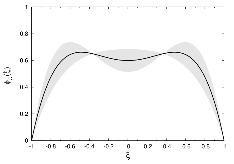
Figure 14: Distribution amplitude of the pion using the expansion in Eq. (3) with our result for $a_{2}^{\pi}=0.201(114)$ and $a_{4}^{\pi}=0$. This result is obtained in the $\overline{\rm MS}$ scheme at $\mu^{2}=4\,\text{GeV}^{2}$. The shaded area indicates the results obtained when $a_{2}^{\pi}$ varies between the maximum and minimum values allowed by its error.

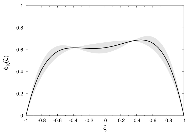
Figure 15: Distribution amplitude of the Kaon using the expansion in Eq. (3) with our results for $a_{1}^{K}=0.0453(9)(29)$ and $a_{2}^{K}=0.175(18)(47)$. These results are obtained in the $\overline{\rm MS}$ scheme at $\mu^{2}=4\,\text{GeV}^{2}$. The shaded area indicates the results obtained when $a_{1}^{K}$ and $a_{2}^{K}$ vary between the maximum and minimum values allowed by their errors.

The coefficients $a_{n}$ in the Gegenbauer expansion of the DAs in Eq. (3) are related to the moments $\langle\xi^{n}\rangle$ by simple agebraic relations (17). Using our result in Eq. (37) we obtain, for the $\pi$-meson

$$a_{2}^{\pi}(\mu^{2}=4~{}\mbox{GeV}^{2})=0.201(114)\,,$$ (43)

and from Eqs. (40) and (42) for the $K$-meson:

$$a_{1}^{K}(\mu^{2} = 4~{}\mbox{GeV}^{2})=0.0453(9)(29)\,,$$ (44)

$$a_{2}^{K}(\mu^{2} = 4~{}\mbox{GeV}^{2})=0.175(18)(47)\,.$$ (45)

While our result for $a_{2}^{\pi}$ is larger than the transverse lattice result Dalley and van de Sande (2003), all three numbers are well within the range suggested by QCD sum rule estimates and supported (for the pion) by the analysis of CLEO data on the $\pi\gamma^{*}\gamma$ transition form factor, cf. Eqs. (11) and (12). Also the $SU(3)$ breaking in the second Gegenbauer coefficient turns out to be small, in agreement with Ball et al. (2006); Khodjamirian et al. (2004). We note that in the context of SU(3) flavour violation, one might be worried about the absence of a dynamical strange quark in our simulations, however there has recently appeared a $N_{f}=2+1$ lattice calculation of $a_{1}^{K}$ Boyle et al. (2006) which is in good agreement with our result, giving us confidence that the effects of a dynamical strange quark are probably small.

Our results indicate that it is important to consider not only the chiral extrapolation of the lattice results to the physical quark masses, but also to perform simulations at small enough lattice spacings to allow for a reliable extrapolation to the continuum limit.

The corresponding DAs obtained by the truncation of the general expression in Eq. (3) after the second term are shown in Fig. 14 and Fig. 15 for the $\pi$ and the $K$-mesons, respectively. Note that the $K$-meson DA is tilted towards larger momentum fractions carried by the heavier strange quark, which is in agreement with general expectations.

In order to illustrate the possible effect of higher-order terms in the Gegenbauer expansion, we also show in Fig. 16 the pion DA obtained with the addition of the fourth-order polynomial with the coefficient $a_{4}^{\pi}=-0.10(5)$ taken from Ref. Bakulev et al. (2006). In both cases (with and without $a_{4}^{\pi}$) the value of the DA in the middle point agrees well with the estimate in Eq. (13). The question whether the “camel-hump” structure of the DA is present in the physical DA depends on the contribution of yet higher-order polynomials that are beyond the reach of the present analysis.

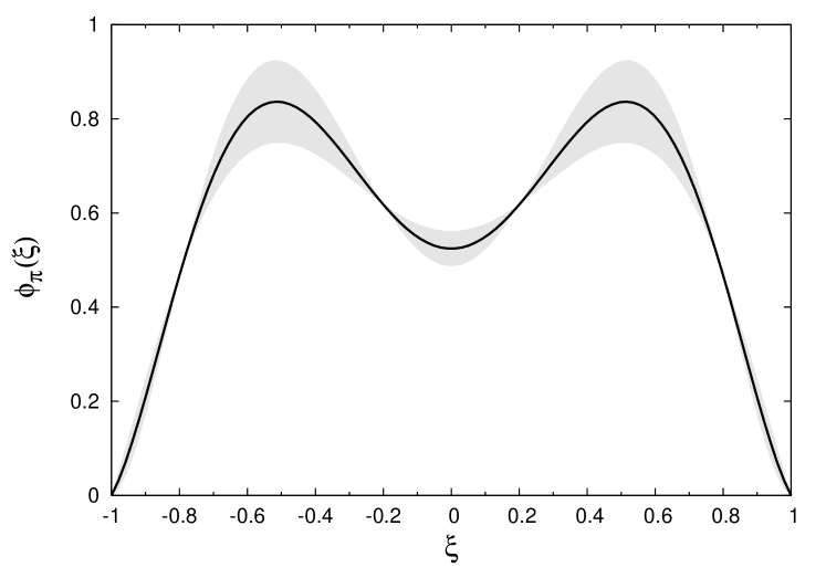
Figure 16: Distribution amplitude of the pion using the expansion in Eq. (3) with $a_{2}^{\pi}=0.201(114)$ and $a_{4}^{\pi}=-0.10(5)$. This result is obtained in the $\overline{\rm MS}$ scheme at $\mu^{2}=4\,\text{GeV}^{2}$. The shaded area indicates the results obtained when we fix $a_{2}^{\pi}$ at its central value and let $a_{4}^{\pi}$ vary between the maximum and minimum values allowed by its error.

Appendix A Lattice results by working point

The following tables summarize our findings at individual working points.

Table 7: Bare results for $\langle\xi\rangle$ and $\langle\xi^{2}\rangle$ for various choices of valences quarks with $\kappa_{\text{val1}}\geq\kappa_{\text{val2}}$, together with the corresponding pseudoscalar mass, $m_{\text{ps}}(\kappa_{\text{val1}},\,\kappa_{\text{val2}})$. Here $\beta=5.29$ and $\kappa_{\text{sea}}=0.13400$.

$\beta=5.29,\ \kappa_{\rm sea}=0.13400$
$\kappa_{\rm val1}$	$\kappa_{\rm val2}$	$am_{\rm ps}$	$\langle\xi\rangle_{a}^{5}$	$\langle\xi\rangle_{a}^{45}$	$\langle\xi\rangle_{b}^{5}$	$\langle\xi\rangle_{b}^{45}$	$\langle\xi^{2}\rangle_{a}^{5}$	$\langle\xi^{2}\rangle_{a}^{45}$
0.13400	0.13400	0.5767(11)	-0.00027(99)	0.0001(11)			0.1434(54)	0.1537(47)
0.13440	0.13400	0.5583(10)	0.0053(10)	0.0059(11)	0.005873(71)	0.005989(92)	0.1445(58)	0.1552(50)
0.13525	0.13400	0.5179(11)	0.0179(14)	0.0190(15)	0.01844(30)	0.01888(40)	0.1468(70)	0.1586(60)
0.13525	0.13440	0.4981(11)	0.0121(14)	0.0131(15)	0.01257(24)	0.01290(32)	0.1475(76)	0.1600(64)
0.13525	0.13525	0.4541(11)					0.1490(94)	0.1636(77)
0.13580	0.13400	0.4906(11)	0.0259(15)	0.0270(17)	0.02666(58)	0.02741(78)	0.1480(83)	0.1607(70)
0.13580	0.13440	0.4700(11)	0.0201(16)	0.0210(18)	0.02080(53)	0.02146(73)	0.1485(90)	0.1621(75)
0.13580	0.13525	0.4237(12)	0.0076(19)	0.0083(20)	0.00826(33)	0.00867(50)	0.149(11)	0.1656(90)
0.13580	0.13580	0.3913(14)					0.150(14)	0.169(11)
0.13630	0.13400	0.4639(15)	0.0332(19)	0.0337(21)	0.0352(14)	0.0367(19)	0.151(11)	0.1633(91)
0.13630	0.13440	0.4423(16)	0.0275(19)	0.0277(22)	0.0294(15)	0.0311(20)	0.153(13)	0.1651(99)
0.13630	0.13525	0.3929(21)	0.0154(23)	0.0150(25)	0.0172(16)	0.0191(27)	0.159(18)	0.171(13)
0.13630	0.13580	0.3569(32)	0.0081(28)	0.0072(29)	0.0093(18)	-0.0009(17)	0.165(35)	0.178(18)
0.13630	0.13630	0.305(14)					0.17(15)	0.183(36)

Table 8: Bare results for $\langle\xi\rangle$ and $\langle\xi^{2}\rangle$ for various choices of valences quarks with $\kappa_{\text{val1}}\geq\kappa_{\text{val2}}$, together with the corresponding pseudoscalar mass, $m_{\text{ps}}(\kappa_{\text{val1}},\,\kappa_{\text{val2}})$. Here $\beta=5.29$ and $\kappa_{\text{sea}}=0.13500$.

$\beta=5.29,\ \kappa_{\rm sea}=0.13500$
$\kappa_{\rm val1}$	$\kappa_{\rm val2}$	$am_{\rm ps}$	$\langle\xi\rangle_{a}^{5}$	$\langle\xi\rangle_{a}^{45}$	$\langle\xi\rangle_{b}^{5}$	$\langle\xi\rangle_{b}^{45}$	$\langle\xi^{2}\rangle_{a}^{5}$	$\langle\xi^{2}\rangle_{a}^{45}$
0.13390	0.13390	0.53134(84)	0.00035(68)	0.00028(78)			0.1332(29)	0.1521(32)
0.13430	0.13390	0.51236(86)	0.00622(70)	0.00647(81)	0.006642(76)	0.006706(75)	0.1336(31)	0.1532(34)
0.13430	0.13430	0.49293(76)	0.00040(73)	0.00028(85)			0.1339(28)	0.1544(28)
0.13500	0.13390	0.47803(88)	0.01731(94)	0.01713(92)	0.01838(28)	0.01850(27)	0.1342(35)	0.1555(38)
0.13500	0.13430	0.45771(90)	0.01078(80)	0.01100(96)	0.01163(20)	0.01179(20)	0.1344(37)	0.1566(40)
0.13500	0.13500	0.42053(82)	0.00049(92)	0.0002(10)			0.1346(37)	0.1587(35)
0.13550	0.13390	0.45254(91)	0.0253(11)	0.02527(98)	0.02657(50)	0.02686(51)	0.1345(40)	0.1573(43)
0.13550	0.13430	0.43142(93)	0.0191(11)	0.0188(10)	0.01996(45)	0.02013(45)	0.1345(42)	0.1587(45)
0.13550	0.13500	0.39249(98)	0.0080(10)	0.0078(12)	0.00833(27)	0.00832(27)	0.1344(47)	0.1602(50)
0.13550	0.13550	0.36283(91)	0.0006(12)	0.0001(13)			0.1344(50)	0.1619(44)
0.13600	0.13390	0.42603(97)	0.0335(13)	0.0335(15)	0.03505(92)	0.03518(93)	0.1346(46)	0.1590(49)
0.13600	0.13430	0.40392(99)	0.0274(14)	0.0271(15)	0.02846(90)	0.02842(92)	0.1344(49)	0.1598(52)
0.13600	0.13500	0.3628(10)	0.0159(12)	0.0157(13)	0.01690(79)	0.01658(86)	0.1339(56)	0.1617(58)
0.13600	0.13550	0.3309(11)	0.0085(14)	0.0079(15)	0.00864(57)	0.00827(71)	0.1332(64)	0.1637(64)
0.13600	0.13600	0.2962(11)	0.0010(18)	0.0006(19)			0.1320(81)	0.1665(65)

Table 9: Bare results for $\langle\xi\rangle$ and $\langle\xi^{2}\rangle$ for various choices of valences quarks with $\kappa_{\text{val1}}\geq\kappa_{\text{val2}}$, together with the corresponding pseudoscalar mass, $m_{\text{ps}}(\kappa_{\text{val1}},\,\kappa_{\text{val2}})$. Here $\beta=5.29$ and $\kappa_{\text{sea}}=0.13550$.

$\beta=5.29,\ \kappa_{\rm sea}=0.13550$
$\kappa_{\rm val1}$	$\kappa_{\rm val2}$	$am_{\rm ps}$	$\langle\xi\rangle_{a}^{5}$	$\langle\xi\rangle_{a}^{45}$	$\langle\xi\rangle_{b}^{5}$	$\langle\xi\rangle_{b}^{45}$	$\langle\xi^{2}\rangle_{a}^{5}$	$\langle\xi^{2}\rangle_{a}^{45}$
0.13430	0.13430	0.46159(55)	-0.0006(8)	-0.0005(10)			0.1484(37)	0.1579(37)
0.13490	0.13430	0.43065(56)	0.0109(9)	0.0110(12)	0.0115(1)	0.0116(2)	0.1510(41)	0.1617(40)
0.13490	0.13490	0.39820(58)	-0.0008(11)	-0.0008(14)			0.1525(45)	0.1645(45)
0.13550	0.13430	0.39837(59)	0.0226(11)	0.0228(14)	0.0234(4)	0.0236(4)	0.1546(47)	0.1670(46)
0.13550	0.13490	0.36397(60)	0.0106(14)	0.0106(17)	0.0118(2)	0.0120(3)	0.1559(52)	0.1698(52)
0.13550	0.13550	0.32696(64)	-0.0020(16)	-0.0019(20)			0.1578(76)	0.1737(68)
0.13585	0.13430	0.37873(62)	0.0293(13)	0.0296(16)	0.0304(6)	0.0306(8)	0.1574(52)	0.1713(53)
0.13585	0.13490	0.34288(64)	0.0166(18)	0.0166(21)	0.0190(5)	0.0190(7)	0.1594(71)	0.1739(66)
0.13585	0.13550	0.30381(67)	0.0045(19)	0.0049(23)	0.0071(3)	0.0071(6)	0.1610(88)	0.1791(78)
0.13585	0.13585	0.27895(72)	-0.0034(22)	-0.0026(27)			0.162(10)	0.1841(91)
0.13620	0.13430	0.35835(74)	0.0355(17)	0.0362(21)	0.0380(13)	0.0382(17)	0.1613(64)	0.1770(66)
0.13620	0.13490	0.32065(78)	0.0220(24)	0.0226(27)	0.0266(13)	0.0269(21)	0.1646(88)	0.1812(83)
0.13620	0.13550	0.27880(88)	0.0098(26)	0.0112(30)	0.0147(12)		0.167(11)	0.1870(97)
0.13620	0.13585	0.2515(11)	0.0038(27)	0.0051(33)			0.168(13)	0.193(11)
0.13620	0.13620	0.2198(26)	-0.0081(56)	-0.0044(51)			0.173(33)	0.201(18)

Table 10: Bare results for $\langle\xi\rangle$ and $\langle\xi^{2}\rangle$ for various choices of valences quarks with $\kappa_{\text{val1}}\geq\kappa_{\text{val2}}$, together with the corresponding pseudoscalar mass, $m_{\text{ps}}(\kappa_{\text{val1}},\,\kappa_{\text{val2}})$. Here $\beta=5.29$ and $\kappa_{\text{sea}}=0.13590$.

$\beta=5.29,\ \kappa_{\rm sea}=0.13590$
$\kappa_{\rm val1}$	$\kappa_{\rm val2}$	$am_{\rm ps}$	$\langle\xi\rangle_{a}^{5}$	$\langle\xi\rangle_{a}^{45}$	$\langle\xi\rangle_{b}^{5}$	$\langle\xi\rangle_{b}^{45}$	$\langle\xi^{2}\rangle_{a}^{5}$	$\langle\xi^{2}\rangle_{a}^{45}$
0.13490	0.13490	0.37239(65)	-0.0005(8)	-0.0021(10)			0.1437(43)	0.1605(38)
0.13530	0.13490	0.34894(67)	0.0078(0)	0.0062(11)	0.0084(1)	0.0084(2)	0.1438(48)	0.1628(42)
0.13530	0.13530	0.32430(69)	-0.0008(12)	-0.0029(14)			0.1441(54)	0.1661(46)
0.13575	0.13490	0.32121(71)	0.0168(12)	0.0156(13)	0.0176(4)	0.0176(6)	0.1434(57)	0.1660(49)
0.13575	0.13530	0.29483(73)	0.0081(14)	0.0066(15)	0.0092(3)	0.0092(4)	0.1432(65)	0.1693(55)
0.13575	0.13575	0.26270(77)	-0.0018(20)	-0.0038(21)			0.1420(79)	0.1740(65)
0.13590	0.13490	0.31158(74)	0.0197(13)	0.0186(15)	0.0205(6)	0.0204(8)	0.1449(74)	0.1672(53)
0.13590	0.13530	0.28450(75)	0.0110(15)	0.0097(17)	0.0121(5)	0.0120(7)	0.1427(71)	0.1705(59)
0.13590	0.13575	0.25123(80)	0.0008(19)	-0.0005(21)	0.0029(2)	0.0028(3)	0.1411(86)	0.1751(71)
0.13590	0.13590	0.23925(82)	-0.0024(25)	-0.0042(26)			0.1401(94)	0.1769(77)
0.13617	0.13490	0.29364(80)	0.0244(17)	0.0238(20)	0.0255(12)	0.0251(16)	0.1447(93)	0.1692(65)
0.13617	0.13530	0.26503(81)	0.0157(19)	0.0149(22)	0.0170(13)	0.0162(17)	0.1407(87)	0.1725(73)
0.13617	0.13575	0.22921(86)	0.0054(25)	0.0047(28)	0.0077(13)		0.139(11)	0.1770(88)
0.13617	0.13590	0.21603(89)	0.0019(28)	0.0013(30)			0.138(12)	0.1787(96)
0.13617	0.13617	0.1897(10)	-0.0042(44)	-0.0044(44)			0.134(15)	0.182(12)

References

- Brodsky and Lepage (1989) S. J. Brodsky and G. P. Lepage, Adv. Ser. Direct. High Energy Phys. 5, 93 (1989).
- Chernyak and Zhitnitsky (1977) V. L. Chernyak and A. R. Zhitnitsky, JETP Lett. 25, 510 (1977).
- Chernyak and Zhitnitsky (1980) V. L. Chernyak and A. R. Zhitnitsky, Sov. J. Nucl. Phys. 31, 544 (1980).
- Efremov and Radyushkin (1980a) A. V. Efremov and A. V. Radyushkin, Phys. Lett. B94, 245 (1980a).
- Efremov and Radyushkin (1980b) A. V. Efremov and A. V. Radyushkin, Theor. Math. Phys. 42, 97 (1980b).
- Lepage and Brodsky (1979) G. P. Lepage and S. J. Brodsky, Phys. Lett. B87, 359 (1979).
- Lepage and Brodsky (1980) G. P. Lepage and S. J. Brodsky, Phys. Rev. D22, 2157 (1980).
- Chernyak et al. (1977) V. L. Chernyak, A. R. Zhitnitsky, and V. G. Serbo, JETP Lett. 26, 594 (1977).
- Chernyak et al. (1980) V. L. Chernyak, V. G. Serbo, and A. R. Zhitnitsky, Sov. J. Nucl. Phys. 31, 552 (1980).
- Stefanis et al. (2000) N. G. Stefanis, W. Schroers, and H.-C. Kim, Eur. Phys. J. C18, 137 (2000), eprint hep-ph/0005218.
- Beneke et al. (2000) M. Beneke, G. Buchalla, M. Neubert, and C. T. Sachrajda, Nucl. Phys. B591, 313 (2000), eprint hep-ph/0006124.
- Keum and Li (2001) Y.-Y. Keum and H.-n. Li, Phys. Rev. D63, 074006 (2001), eprint hep-ph/0006001.
- Bauer et al. (2001) C. W. Bauer, S. Fleming, D. Pirjol, and I. W. Stewart, Phys. Rev. D63, 114020 (2001), eprint hep-ph/0011336.
- Bauer et al. (2002) C. W. Bauer, D. Pirjol, and I. W. Stewart, Phys. Rev. D65, 054022 (2002), eprint hep-ph/0109045.
- Ball and Braun (1998) P. Ball and V. M. Braun, Phys. Rev. D58, 094016 (1998), eprint hep-ph/9805422.
- Khodjamirian et al. (2000) A. Khodjamirian, R. Ruckl, S. Weinzierl, C. W. Winhart, and O. I. Yakovlev, Phys. Rev. D62, 114002 (2000), eprint hep-ph/0001297.
- Ball and Zwicky (2005a) P. Ball and R. Zwicky, Phys. Rev. D71, 014029 (2005a), eprint hep-ph/0412079.
- Eidelman et al. (2004) S. Eidelman et al. (Particle Data Group), Phys. Lett. B592, 1 (2004).
- Brodsky et al. (1980) S. J. Brodsky, Y. Frishman, G. P. Lepage, and C. T. Sachrajda, Phys. Lett. B91, 239 (1980).
- Ohrndorf (1982) T. Ohrndorf, Nucl. Phys. B198, 26 (1982).
- Braun et al. (2003) V. M. Braun, G. P. Korchemsky, and D. Müller, Prog. Part. Nucl. Phys. 51, 311 (2003), eprint hep-ph/0306057.
- Makeenko (1981) Y. M. Makeenko, Sov. J. Nucl. Phys. 33, 440 (1981).
- Mikhailov and Radyushkin (1985) S. V. Mikhailov and A. V. Radyushkin, Nucl. Phys. B254, 89 (1985).
- Mueller (1994) D. Mueller, Phys. Rev. D49, 2525 (1994).
- Mueller (1995) D. Mueller, Phys. Rev. D51, 3855 (1995), eprint hep-ph/9411338.
- Mertig and van Neerven (1996) R. Mertig and W. L. van Neerven, Z. Phys. C70, 637 (1996), eprint hep-ph/9506451.
- Bakulev et al. (2004) A. P. Bakulev, K. Passek-Kumericki, W. Schroers, and N. G. Stefanis, Phys. Rev. D70, 033014 (2004), eprint hep-ph/0405062.
- Chernyak and Zhitnitsky (1982) V. L. Chernyak and A. R. Zhitnitsky, Nucl. Phys. B201, 492 (1982).
- Chernyak and Zhitnitsky (1984) V. L. Chernyak and A. R. Zhitnitsky, Phys. Rept. 112, 173 (1984).
- Stefanis et al. (1999) N. G. Stefanis, W. Schroers, and H.-C. Kim, Phys. Lett. B449, 299 (1999), eprint hep-ph/9807298.
- Ball et al. (2006) P. Ball, V. M. Braun, and A. Lenz (2006), eprint hep-ph/0603063.
- Bakulev et al. (2003) A. P. Bakulev, S. V. Mikhailov, and N. G. Stefanis, Phys. Rev. D67, 074012 (2003), eprint hep-ph/0212250.
- Khodjamirian et al. (2004) A. Khodjamirian, T. Mannel, and M. Melcher, Phys. Rev. D70, 094002 (2004), eprint hep-ph/0407226.
- Braun and Lenz (2004) V. M. Braun and A. Lenz, Phys. Rev. D70, 074020 (2004), eprint hep-ph/0407282.
- Ball and Zwicky (2006a) P. Ball and R. Zwicky, Phys. Lett. B633, 289 (2006a), eprint hep-ph/0510338.
- Ball and Zwicky (2006b) P. Ball and R. Zwicky, JHEP 02, 034 (2006b), eprint hep-ph/0601086.
- Schmedding and Yakovlev (2000) A. Schmedding and O. I. Yakovlev, Phys. Rev. D62, 116002 (2000), eprint hep-ph/9905392.
- Bakulev et al. (2006) A. P. Bakulev, S. V. Mikhailov, and N. G. Stefanis, Phys. Rev. D73, 056002 (2006), eprint hep-ph/0512119.
- Agaev (2005) S. S. Agaev, Phys. Rev. D72, 114010 (2005), eprint hep-ph/0511192.
- Ball and Zwicky (2005b) P. Ball and R. Zwicky, Phys. Lett. B625, 225 (2005b), eprint hep-ph/0507076.
- Bakulev et al. (2001) A. P. Bakulev, S. V. Mikhailov, and N. G. Stefanis, Phys. Lett. B508, 279 (2001), eprint hep-ph/0103119.
- Dalley and van de Sande (2003) S. Dalley and B. van de Sande, Phys. Rev. D67, 114507 (2003), eprint hep-ph/0212086.
- Capitani et al. (1999) S. Capitani et al., Nucl. Phys. Proc. Suppl. 79, 173 (1999), eprint hep-ph/9906320.
- Detmold and Lin (2006) W. Detmold and C. J. D. Lin, Phys. Rev. D73, 014501 (2006), eprint hep-lat/0507007.
- Braun and Filyanov (1989) V. M. Braun and I. E. Filyanov, Z. Phys. C44, 157 (1989).
- Aitala et al. (2001) E. M. Aitala et al. (E791), Phys. Rev. Lett. 86, 4768 (2001), eprint hep-ex/0010043.
- Braun et al. (2001) V. M. Braun, D. Y. Ivanov, A. Schäfer, and L. Szymanowski, Phys. Lett. B509, 43 (2001), eprint hep-ph/0103275.
- Braun et al. (2002) V. M. Braun, D. Y. Ivanov, A. Schäfer, and L. Szymanowski, Nucl. Phys. B638, 111 (2002), eprint hep-ph/0204191.
- Chernyak (2001) V. Chernyak, Phys. Lett. B516, 116 (2001), eprint hep-ph/0103295.
- Chernyak and Grozin (2001) V. L. Chernyak and A. G. Grozin, Phys. Lett. B517, 119 (2001), eprint hep-ph/0106162.
- Kronfeld and Photiadis (1985) A. S. Kronfeld and D. M. Photiadis, Phys. Rev. D31, 2939 (1985).
- Martinelli and Sachrajda (1987) G. Martinelli and C. T. Sachrajda, Phys. Lett. B190, 151 (1987).
- Daniel et al. (1991) D. Daniel, R. Gupta, and D. G. Richards, Phys. Rev. D43, 3715 (1991).
- Del Debbio et al. (2000) L. Del Debbio, M. Di Pierro, A. Dougall, and C. T. Sachrajda (UKQCD), Nucl. Phys. Proc. Suppl. 83, 235 (2000), eprint hep-lat/9909147.
- Del Debbio et al. (2003) L. Del Debbio, M. Di Pierro, and A. Dougall, Nucl. Phys. Proc. Suppl. 119, 416 (2003), eprint hep-lat/0211037.
- Göckeler et al. (2005a) M. Göckeler et al. (2005a), eprint hep-lat/0510089.
- Best et al. (1997) C. Best et al., Phys. Rev. D56, 2743 (1997), eprint hep-lat/9703014.
- Göckeler et al. (2006a) M. Göckeler et al. (2006a), eprint hep-lat/0605002.
- Capitani et al. (2001) S. Capitani et al., Nucl. Phys. B593, 183 (2001), eprint hep-lat/0007004.
- Göckeler et al. (2005b) M. Göckeler et al., Nucl. Phys. B717, 304 (2005b), eprint hep-lat/0410009.
- Aubin et al. (2004) C. Aubin et al., Phys. Rev. D70, 094505 (2004), eprint hep-lat/0402030.
- Khan et al. (2006) A. A. Khan et al. (2006), eprint hep-lat/0603028.
- Göckeler et al. (2006b) M. Göckeler et al., Phys. Rev. D73, 014513 (2006b), eprint hep-ph/0502212.
- Göckeler et al. (2005c) M. Göckeler, R. Horsley, D. Pleiter, P. E. L. Rakow, and G. Schierholz (QCDSF), Phys. Rev. D71, 114511 (2005c), eprint hep-ph/0410187.
- Martinelli et al. (1995) G. Martinelli, C. Pittori, C. T. Sachrajda, M. Testa, and A. Vladikas, Nucl. Phys. B445, 81 (1995), eprint hep-lat/9411010.
- Göckeler et al. (1999) M. Göckeler et al., Nucl. Phys. B544, 699 (1999), eprint hep-lat/9807044.
- Göckeler et al. (2005d) M. Göckeler et al., Phys. Rev. D72, 054507 (2005d), eprint hep-lat/0506017.
- Chen and Stewart (2004) J.-W. Chen and I. W. Stewart, Phys. Rev. Lett. 92, 202001 (2004), eprint hep-ph/0311285.
- Chen et al. (2006) J.-W. Chen, H.-M. Tsai, and K.-C. Weng, Phys. Rev. D73, 054010 (2006), eprint hep-ph/0511036.
- Boyle et al. (2006) P. A. Boyle et al. (2006), eprint hep-lat/0607018.
- Allton et al. (2002) C. R. Allton et al. (UKQCD), Phys. Rev. D65, 054502 (2002), eprint hep-lat/0107021.