DESY-06-080

HU-EP-06/14

SFB/CPP-06-26

Exploring the HMC trajectory-length dependence
of autocorrelation times in lattice QCD

Harvey Meyer, Hubert Simma, Rainer Sommer

Deutsches Elektronen Synchrotron DESY

Platanenallee 6

D-15738 Zeuthen

Michele Della Morte, Oliver Witzel, Ulli Wolff

Humboldt-Universität, Institut für Physik

Newtonstrasse 15

D-12489 Berlin

Abstract
We study autocorrelation times of physical observables in lattice QCD as a function of the molecular dynamics trajectory length in the hybrid Monte-Carlo algorithm. In an interval of trajectory lengths where energy and reversibility violations can be kept under control, we find a variation of the integrated autocorrelation times by a factor of about two in the quantities of interest. Trajectories longer than conventionally used are found to be superior both in the $\mathop{N_{\rm f}=0}$ and $\mathop{N_{\rm f}=2}$ examples considered here. We also provide evidence that they lead to faster thermalization of systems with light quarks.

1 Introduction

Hybrid Monte-Carlo (HMC) [1] is the most widely used algorithm to simulate non-Abelian gauge theories in the presence of $N_{f}>0$ quark flavours. For Wilson-type quark actions it was found, in its most straightforward application, to become prohibitively expensive in the regime of phenomenological interest (with two very light quarks) [2]. Recent advances [3, 4, 5, 6] however have led to a substantial lowering of the CPU time of simulations. These more sophisticated forms of HMC typically have a number of parameters that have to be tuned to guarantee an efficient simulation. One parameter that is however common to all HMC algorithms is the length $\tau$ of the trajectories of ‘molecular dynamics’ evolution, at the end of which an accept/reject step is performed to correct for any finite-step-size errors.

The algorithm efficiency’s dependence on $\tau$ has only been rarely and partially studied in the literature [7, 8, 9, 10]. The reason for this is easy to understand. If we neglect the cost of evaluating the Hamiltonian, performing trajectories of length $\tau=2$ represents the same computational cost as twice as many trajectories of length $1$: indeed, as discussed in the appendix, the average energy violations along a trajectory at fixed step-size are weakly dependent on the length within a reasonable range, and the reversibility violations increase rather slowly (see however [12]). Hence, with a high acceptance rate in both cases, to discriminate between these two running modes one has to determine the autocorrelation times of the observables of interest with some accuracy and reliability. This in turn requires very high statistics, which one is normally not ready to invest into parameter optimization. In this letter we study this question in various situations where high statistics can be achieved, and yet some realistic features of difficult simulations are present.

Whether in the end our conclusions carry over to other forms of HMC algorithms will require direct testing. However we show that the dependence of the algorithm’s efficiency on $\tau$ can be significant, and a factor around two in computing time can easily be wasted in the case of an unfortunate choice of trajectory length.

2 Data

We employ the hybrid Monte-Carlo algorithm [1]. The Hamiltonian governing the evolution of the molecular dynamics is

$$H={\textstyle{\frac{1}{2}}}\sum_{\mu,x}{\rm Tr\,}\{\Pi_{\mu}(x)\Pi_{\mu}(x)\}+S[U].$$ (1)

where the momenta $\Pi_{\mu}$ are traceless Hermitian matrices. The gauge fields are thus updated according to $U^{\prime}_{\mu}(x)=\exp[i\Pi_{\mu}(x)d\tau]U_{\mu}(x)$. In the $\mathop{N_{\rm f}=2}$ simulations, two pseudofermions are used to stochastically represent the determinant of the O($a$) improved Wilson fermions: the fermionic part of $S$ results from even-odd- [11] and mass-preconditioning [4] the Hermitian Dirac operator. The gauge part of $S$ is the Wilson plaquette action.

When $\mathop{N_{\rm f}=2}$, we use the Sexton-Weingarten integration scheme [13], with a step-size four times larger for the fermionic forces; the quoted step-size $d\tau$ always denotes the largest one. A complete update cycle with trajectory length $\tau$ performs an integer number $\tau/d\tau$ of such steps followed by the Metropolis decision. The system has then advanced by $\tau$ molecular dynamics (MD) units, and in the rest of this paper all quantities referring to Monte Carlo time are given in MD units. If for instance successive measurements of observables are separated by $M$ trajectories, an autocorrelation function $\Gamma(i)$ arises where $i$ refers to successive measurements. From it we define the integrated autocorrelation time, that is directly relevant for the statistical error, in our MD units as

$$\mathop{\tau_{\rm int}}=M\tau{\textstyle\left[\frac{1}{2}+\sum_{i\geq 1}\rho(i)\right]},\qquad\rho(i)=\Gamma(i)/\Gamma(0).$$ (2)

In numerical estimates the sum has to be truncated. If we specify a window $W$ (in MD units) this amounts to the restriction $i\leq W/(M\tau)$. We refer the reader to [14] for the definition of $\Gamma(i)$, in particular for derived quantities, such as an effective mass. The error bars shown in plots of $\rho$ are computed using Eq. (E.11) of reference [3].

We investigate the trajectory length dependence of autocorrelation times in three different systems (A,B,C: see Tab. 1). All simulations were done in 32-bit arithmetic, except for system C (64-bit). The system D will be used as a playground for thermalization. The lattice spacing is known in units of $r_{0}$ [17] at $1\%$ level for the $N_{f}=0$ runs and $5\%$ for the $\mathop{N_{\rm f}=2}$ runs. All lattices have Schrödinger functional boundary conditions. Since we will be using somewhat longer trajectories than is usual, the question of reversibility violations arises. We check for this in the standard way (see e.g. [7]) by monitoring the Hamiltonian variation $\langle|\delta H|_{\leftrightarrow}\rangle$ under the following operations : a trajectory ‘forward’, reversing the sign of the momenta, and integrating back to the starting point.

	$L^{3}\times T$	BF	$N_{\rm f}$	$1/d\tau$	$\beta$	$\kappa$	$a/r_{0}$ [ref]	$a\mathop{M_{\rm PS}}$
A	$8^{4}$	$A$	0	30	$6.086$	-	0.16 [21]	-
	$12^{4}$	$A$	0	30	$6.364$	-	0.11 [21]	-
	$16^{4}$	$A$	0	30	$6.57$	-	0.08 [21]	-
B	$8^{3}\times 32$	0	0	50	6.0	0.1338	0.19 [21]	0.38(2)
C	$24^{3}\times 32$	0	2	32	5.3	0.1355	0.16 [23]	0.325(10)
D	$12^{4}$	$A\to 0$	2	32	5.6215	0.136665	0.11 [22]	-

Table 1: The parameters of the physical systems considered. A boundary field (BF) 0 means that it is vanishing, while $A$ refers to ‘point $A$’ of Ref. [16].

The observables we will focus on are those which typically have autocorrelation times much larger than that of the plaquette. One observable (defined already in the pure gauge theory) is $dS/d\eta$; the inverse of its expectation value defines the Schrödinger functional renormalized coupling constant [16]. The others are fermionic: the correlators $f_{\rm A}(x_{0})$ and $f_{\rm P}(x_{0})$ correspond to the propagation of a quark and an antiquark from a boundary to a point in the bulk of the lattice where the axial current or pseudoscalar density annihilates them [15]. Finally we also consider $f_{1}$, which is the amplitude for boundary-to-boundary propagation through the lattice. It serves to normalize the other correlators. In particular, $Z_{\rm A}f_{\rm A}(x_{0})/\sqrt{f_{1}}\sim\mathop{F_{\rm PS}}e^{-(x_{0}-T/2)\mathop{M_{\rm PS}}}$ holds far from the boundaries, where $\mathop{M_{\rm PS}}$ and $\mathop{F_{\rm PS}}$ correspond to the pseudoscalar mass and decay constant [15].

2.1 HMC in the pure gauge theory

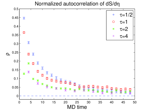
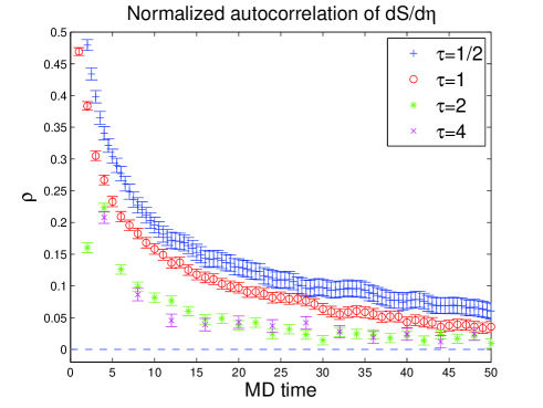
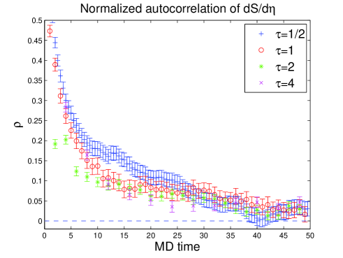
Figure 1: Autocorrelation function of $dS/d\eta$ in a pure gauge HMC (system A), for different trajectory lengths (from top to bottom: $L=8,12$ and 16).

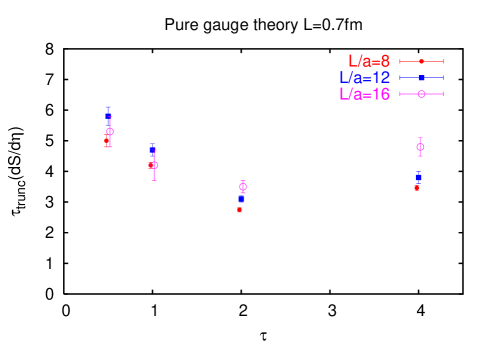
Figure 2: The truncated autocorrelation time of $dS/d\eta$ in the pure gauge system (A), as a function of the trajectory length $\tau$ and for different lattice spacings.

A: pure gauge	$\tau=1/2$	$\tau=1$	$\tau=2$	$\tau=4$
$L=8$ $\tau_{\rm int}[dS/d\eta]$	$6.10(35)_{W=64}$	$5.90(30)_{W=36}$	$3.14(10)_{W=36}$	$3.92(12)_{W=44}$
$\tau_{\rm trunc}[dS/d\eta]_{W=25}$	5.0(2)	4.2(1)	2.75(7)	3.46(9)
Acceptance $[\%]$	97	97	97	96
$\langle\delta H^{2}\rangle/(Ld\tau)^{4}$	0.789(6)	0.953(6)	1.221(8)	1.71(1)
$10^{4}\cdot\langle|\delta H|_{\leftrightarrow}\rangle$	2.0	2.6	3.5	4.9
$L=12$ $\tau_{\rm int}[dS/d\eta]$	$9.5(1.0)_{W=86}$	$6.4(5)_{W=63}$	$3.34(18)_{W=34}$	$4.36(24)_{W=44}$
$\tau_{\rm trunc}[dS/d\eta]_{W=25}$	5.8(3)	4.7(2)	3.1(1)	3.8(2)
Acceptance $[\%]$	94	93	93	91
$\langle\delta H^{2}\rangle/(Ld\tau)^{4}$	0.941(6)	1.134(8)	1.40(1)	1.92(3)
$10^{4}\cdot\langle|\delta H|_{\leftrightarrow}\rangle$	5.1	6.4	8.8	12.2
$L=16$ $\tau_{\rm int}[dS/d\eta]$	$6.5(1.0)_{W=52}$	$5.8(6)_{W=52}$	$4.2(4)_{W=40}$	$6.0(4)_{W=68}$
$\tau_{\rm trunc}[dS/d\eta]_{W=25}$	5.3(5)	4.2(5)	3.5(2)	4.8(3)
Acceptance $[\%]$	89	88	86	84
$\langle\delta H^{2}\rangle/(Ld\tau)^{4}$	1.08(1)	1.31(2)	1.58(2)	2.10(4)
$10^{4}\cdot\langle|\delta H|_{\leftrightarrow}\rangle$	9.1	12	16	21

Table 2: The autocorrelation times (in units of MD time) for $dS/d\eta$, the acceptance, the energy and reversibility violations for different choices of trajectory length. $W$ is the window in MD time over which the autocorrelation time has been accumulated. From top to bottom: $L=8,12$ and 16, while $La/r_{0}$=const. Runs in single precision.

We start by investigating autocorrelation times for gluonic quantities in the pure-gauge HMC (system A), where we have three different lattice spacings at constant physical parameters (see Tab. 2). The acceptance rates, as well as $\langle\delta H^{2}\rangle$, are given (the step-size is the same in all these runs); we are clearly in the regime of high acceptance $P_{A}$ where $\langle\delta H^{2}\rangle\simeq 2\pi(1-P_{A})^{2}$ [26]. The dependence of $\langle\delta H^{2}\rangle$ on $\tau$ is moderate. Therefore the dependence of $P_{A}$ is even weaker, but note that the effect of lower acceptance at larger $\tau$ is automatically taken into account in the autocorrelation of observables. The reversibility violations as measured by $\langle|\delta H|_{\leftrightarrow}\rangle$ grow as $\sqrt{\tau}$ here, or even more slowly; the reader is referred to the appendix for a more detailed discussion of $\langle\delta H^{2}\rangle$ and $\langle|\delta H|_{\leftrightarrow}\rangle$. We now focus on the observable $dS/d\eta$ defined in [16]. We emphasize that, unlike the plaquette, this is an observable dominated by long-distance fluctuations and it typically has an autocorrelation time significantly larger than one.

The most direct way to evaluate the performance of different $\tau$-choices for a given observable is to compare the corresponding normalized autocorrelation function, $\rho(t)$. This is done on Fig. 1, for trajectory lengths $1/2$, 1, 2, 4. There is a marked difference between, say, $\tau=1/2$ and $\tau=2$ in favour of the latter, at all MD-time separations. The choice $\tau=4$ is slightly superior to $\tau=2$ at short MD-time separation at the largest lattice spacing, while the opposite is true at the finest lattice spacing. Note in particular that at the shortest time separation, $\rho$ is much smaller for $\tau=2$ than for $\tau\leq 1$. In fact, the $\tau=2$ autocorrelation function shows a significant non-monotonic behaviour, as we have observed previously only for hybrid overrelaxation algorithms.

For a run of given MD-time length and measurement frequency, the error squared of the observable is proportional to $1/\tau_{\rm int}$. When $\tau_{\rm int}$ is large compared to the measurement frequency, it corresponds to the area under the curves shown in Fig. 1. In practice, a window $W$ must be chosen where to stop the summation. This may be chosen in a self-consistent way which balances statistical against systematic errors. We use by default the prescription described in [14]. However, to rate relative performances of algorithms, we also compute here an integrated autocorrelation time $\tau_{\rm trunc}$ where the summation is truncated at a fixed window $W=25$. It turns out that typically $80\%$ of the true $\tau_{\rm int}$ has by then been accumulated; the uncertainty on $\tau_{\rm trunc}$ is almost half of that on the full $\tau_{\rm int}$ and the hierarchy between the different trajectory lengths is at any rate maintained (Tab. 2).

Fig. 2 then illustrates the dependence of the truncated autocorrelation time on the trajectory length $\tau$. One sees that this quantity is minimized somewhere around $\tau=2$, and this conclusion is largely independent of the lattice spacing in the range considered. Overall we see a variation by a factor two of $\tau_{\rm trunc}$ for $1/2\leq\tau\leq 4$. Generally speaking this is a substantial variation which translates directly into a corresponding speed-up of simulations whose cost is dominated by the HMC.

2.2 HMC in quenched QCD

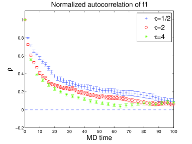
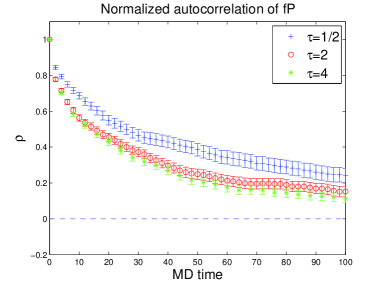
Figure 3: Autocorrelation function of the correlators $f_{1}$ and $f_{\rm P}$ in quenched QCD (system B), for different trajectory lengths.

B: quenched, $8^{3}\times 32$	$\tau=1/2$	$\tau=2$	$\tau=4$
$\tau_{\rm int}[f_{1}]$	$40(5)_{W=270}$	$24(4)_{W=184}$	$20(3)_{W=172}$
$\tau_{\rm int}[f_{\rm P}]$	$75(20)_{W=245}$	$44(8)_{W=316}$	$32(4)_{W=256}$
$\tau_{\rm int}[m_{\rm PS}^{\rm eff}(T/2)]$	25(4)	13.5(1.6)	12.1(1.2)
$\tau_{\rm int}[f_{\rm PS}^{\rm eff}(T/2)]$	33(6)	19.0(2.6)	14.7(1.6)
Acceptance $[\%]$	98	98	97
$\langle\delta H^{2}\rangle/(L^{3}Td\tau^{4})$	0.827(5)	1.32(1)	1.87(3)
$10^{4}\cdot\langle|\delta H|_{\leftrightarrow}\rangle$	4.9	9.9	11

Table 3: The autocorrelations time (in units of MD time) of two primary observables ($f_{1}$ and $f_{\rm P}$) and of the effective pseudoscalar mass and decay constant in the middle of the lattice, the acceptance, the energy and reversibility violations for different choices of trajectory length. Runs in single precision.

As our next observables we now consider fermionic correlators. Although we are ultimately interested in dynamical, large-volume simulations (system C), we first investigate the autocorrelation times in system B, which, roughly speaking, is a quenched version of system C with in addition the spatial extent divided by 3. The computing time is now dominated by the measurements. The run-length is $t_{\rm run}\simeq 32000$ in total (four independent lattices, called ‘replica’, were simulated). We investigate the range $\tau=1/2$ to $\tau=4$, within which we see hardly any variation of the acceptance, and $\langle|\delta H|_{\leftrightarrow}\rangle$ scales roughly with $\sqrt{\tau}$: Tab. 3 shows this, as well as some relevant autocorrelation times.

The comparison of autocorrelation functions for $f_{1}$ and $f_{\rm P}$ is done on Fig. 3. The advantage of $\tau=4$ and $\tau=2$ over $\tau=1/2$ is both substantial and statistically significant. This is reflected in a factor of about two in the integrated autocorrelation times. This gain is at least as marked in physical quantities such as the effective pseudoscalar mass and decay constant.

2.3 Mass-preconditioned HMC in $\mathop{N_{\rm f}=2}$ QCD

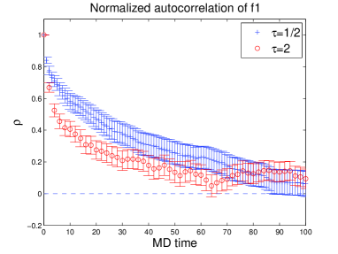
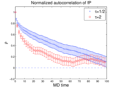
Figure 4: Autocorrelation function of the correlators $f_{1}$ and $f_{\rm P}$ in $\mathop{N_{\rm f}=2}$ QCD (system C), for different trajectory lengths.

C: $\mathop{N_{\rm f}=2},~{}\kappa=0.1355$	$\tau=1/2$	$\tau=2$
$\tau_{\rm int}[f_{1}]$	$30(15)_{W=145}$	$24(8)_{W=134}$
$\tau_{\rm trunc}[f_{1}]_{W=50}$	23(5)	15(3)
$\tau_{\rm int}[f_{\rm P}]$	$45(20)_{W=185}$	$26(10)_{W=134}$
$\tau_{\rm trunc}[f_{\rm P}]_{W=50}$	28(7)	18(4)
$\tau_{\rm int}[m_{\rm PS}^{\rm eff}(T/2)]$	9.5(2.5)	6.8(1.5)
$\tau_{\rm int}[f_{\rm PS}^{\rm eff}(T/2)]$	14(4)	4.2(8)
Acceptance $[\%]$	90	91
$\langle\delta H^{2}\rangle/(L^{3}Td\tau^{4})$	$0.147(4)^{*}$	0.164(6)
$10^{4}\cdot\langle|\delta H|_{\leftrightarrow}\rangle$	1.0	2.5

Table 4: The autocorrelations time (in units of MD time) of two primary observables ($f_{1}$ and $f_{\rm P}$) and of the effective pseudoscalar mass and decay constant in the middle of the lattice, the acceptance, the energy and reversibility violations for different choices of trajectory length. The value of $\langle\delta H^{2}\rangle/(L^{3}Td\tau^{4})$ marked by a ^∗ was obtained for one of the replica; the other had one spike of $\delta H\simeq 2000$. Runs in double precision.

We now come to $\mathop{N_{\rm f}=2}$ dynamical simulations in a spatial volume of $(2{\rm fm})^{3}$, and consider the same fermionic correlators as in the previous section. The quark mass is around $m_{s}$, the strange quark mass, and we have two values of $\tau$, $1/2$ and 2. The total statistics in each case is about $t_{\rm run}=4000$ (2 replica were simulated).

Note that the acceptance is practically the same in both runs. The autocorrelation functions of $f_{1}$ and $f_{\rm P}$ are compared on Fig. 4. Naturally the error bars are now larger; nonetheless a statistically significant advantage of the run at $\tau=2$ is seen at MD-time separations up to about 30. This is confirmed when one looks at the truncated autocorrelation time with a window of $W=50$. The autocorrelation function of $f_{1}$ is in fact surprisingly similar with that in the quenched simulation, Fig. 3. The resulting autocorrelation times are given in Tab. 4. In spite of large uncertainties, there is a significant reduction of $\tau_{\rm int}[f_{\rm PS}^{\rm eff}(T/2)]$ when going from $\tau=1/2$ to $\tau=2$.

2.3.1 Thermalization with light quarks

Since we observe that autocorrelation times of long-distance observables are reduced by the use of longer trajectories, we also expect their thermalization to be accelerated by the latter. Consider the thermalization of system D (see Tab. 1). The exercise here is to

1. start from the ensemble with non-zero boundary field (‘point A’ of [16]);

2. revert to homogeneous Dirichlet boundary conditions, and hence vanishing background field [16];

3. let the system rethermalize under the HMC evolution, for two different choices of trajectory length;

4. track how fast quantities whose expectation values vanish by symmetry in the homogeneous Dirichlet case relax to zero.

Fig. 5 shows the relaxation of the observables $dS/d\eta$ and $f_{\rm P}-f_{\rm P}^{\prime}$. The latter is the asymmetry between the correlator emanating from one boundary and the other. A data point at time $t$ shows the value of the observable averaged over 16 independent replica (corresponding to independent starting configurations), and averaged over the MD time interval $]t-6,t+6]$. The $dS/d\eta$ measurements were done after every trajectory and $f_{\rm P}-f_{\rm P}^{\prime}$ every other trajectory.

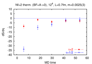
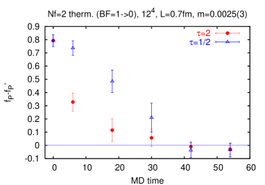
Figure 5: Thermalization of two long-distance observables ($dS/d\eta$ and $f_{\rm P}-f_{\rm P}^{\prime}$) having zero as expectation value. The starting configurations are taken from an ensemble where these expectation values are non-zero (system D).

The thermalization takes place faster with the choice of trajectory length $\tau=2$, at least in the relatively early stages. In difficult simulations the time-consuming part is presumably the tail of the thermalization, but it would require very large statistics to demonstrate an algorithmic advantage in that regime.

3 Conclusion

We have investigated the dependence of autocorrelation times on the HMC trajectory length, focusing on long-distance observables, in a variety of different physical situations. We find this dependence to be substantial (a factor around 2) and statistically significant. The reduced correlation of successive measurements, done at fixed intervals of molecular dynamics time, is most clearly seen in the autocorrelation functions themselves. This means that a reasonable tuning of the trajectory length may save a factor of about 2 in computing time.

The optimal choice of $\tau$ is observable dependent. However we have observed that trajectories longer than the ones conventionally used provide an advantage in computing standard physical quantities such as the pseudoscalar mass and decay constant. It will be interesting to see whether this conclusion also holds for HMC algorithms that use a different preconditioning of the pseudofermion action, for a different number of flavours, etc.

Naturally, other criteria are relevant in the final choice of trajectory length; the issues of stability and reversibility violations have been addressed in the appendix (see also Ref. [7, 12, 24] to name a few). We are currently performing a simulation at a quark mass of $m_{s}/2$ with $\tau=2$ that shows good stability and controlled reversibility violations.

Appendix: Stability and reversibility violations

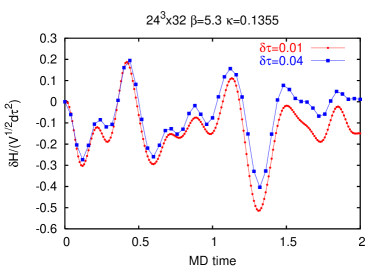
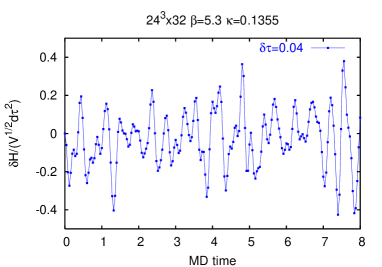
Figure 6: Variation of the Hamiltonian along one MD trajectory on lattice C, in units of $\sqrt{V}d\tau^{2}$, where $V$ is the number of lattice points.

In this appendix we discuss some important issues that one might worry about if one increases the length of MD trajectories. Most of what follows is not new but we find it useful to gather here the relevant points.

Energy violations along a trajectory

Fig. 6 shows the variation of the Hamiltonian along one MD trajectory on lattice C, for two different step sizes (here the leap-frog integrator was used with a ratio of 5 between the time-steps of the two pseudo-fermion forces [5]). The right plot illustrates the fact that the fluctuations of $\delta H(t)$ around zero do not grow very fast with MD time $t$.

Although a symplectic integrator such as leap-frog has discretization errors, there is a Hamiltonian which differs by O$(d\tau^{2})$ terms from the MD Hamiltonian, and which is exactly conserved by the MD evolution [18, 25]:

$$H_{\rm o}=H(t)+d\tau^{2}h_{1}(t)+d\tau^{4}h_{2}(t)+\dots$$ (3)

Hence, for a given start configuration and momenta,

$$-\frac{\delta H(t)}{d\tau^{2}}=\delta h_{1}(t)+d\tau^{2}\delta h_{2}(t)+\dots$$ (4)

In words, the curve $\delta H(t)/d\tau^{2}$ is independent of $d\tau$, up to O$(d\tau^{2})$ corrections. This is clearly what is seen on the left plot of Fig. 6. Note that since in equilibrium $\langle\delta H\rangle\simeq 1/2\langle\delta H^{2}\rangle={\rm O}(d\tau^{4})>0$ holds, we have $\langle\delta h_{1}(t)\rangle=0$ and $\langle\delta h_{2}(t)\rangle<0$ for any fixed $t$.

Scaling of energy violations

The scaling law $\langle\delta H^{2}\rangle\sim Vd\tau^{4}$ was proposed in [18, 19]. Indeed, since $\delta H$ is O$(d\tau^{2})$ for one trajectory, $\delta H^{2}$ is O$(d\tau^{4})$ and so is its average. As to the volume dependence, we confirm that $\langle\delta H^{2}\rangle$ depends mainly on the number of lattice points $V$ [20], while the dependence on the coupling $\beta$ is very weak. The values of $\langle\delta H^{2}\rangle$ in Tab. 2 are consistent with $\langle\delta H^{2}\rangle\propto V^{\eta(\tau)}$, where $\eta\in[1.07,1.11]$.

The dependence of $\langle\delta H^{2}\rangle$ on the trajectory length $\tau$ is very moderate but follows no obvious formula (see Tab. 2). Nevertheless, the trend is reasonably well described by $\tau^{\alpha}$, $0.3<\alpha<0.4$.

Stability

Of course the statements made in the previous paragraph hold for exact arithmetics, and in practice it must be checked empirically at what trajectory length rounding errors introduce instabilities in the integration [24]. The other source of instability can be the occurrence of an exceptionally large force, which spoils the expansion in $d\tau$. In the simulation C (see Tab. 1), $|\delta H|$ was bounded by 1 in the $\tau=2$ run, while one replicum experienced one spike of $\delta H\simeq 2000$ in the $\tau=1/2$ run (the simulation then continued normally).

Reversibility violations

Reversibility violations in our simulations come from rounding errors, and from the non-zero residuals of the inversions in the MD evolution. These effects of course accumulate with the length of the trajectory. However Tab. 2, 3 and 4 show that the increase of $\langle|\delta H_{\leftrightarrow}|\rangle$ with $\tau$ in simulations where $|\delta H|$ is bounded by one and is typically much smaller, is rather slow, roughly like $\sim\sqrt{\tau}$. Therefore it should not present a serious problem. In the trajectory of Fig. 6 with $d\tau=0.04$, $10^{4}\cdot\langle|\delta H|_{\leftrightarrow}\rangle$ is 0.06, 0.3, 1.4 and 1.4 for $\tau=0.08$, 0.8, 1.6 and 8 respectively.

How a small reversibility violation influences the ensemble generated is not known (to us); it may lead to an incorrect sampling. The influence on expectation values of observables is even harder to pin down. The study [7] showed that even with $\langle|\delta H_{\leftrightarrow}|\rangle=0.01$ one does not see an effect in a number of observables computed at the sub-percent level.

References

- [1] S. Duane, A. D. Kennedy, B. J. Pendleton and D. Roweth, Phys. Lett. B 195 (1987) 216.
- [2] A. Ukawa [CP-PACS and JLQCD Collaborations], Nucl. Phys. Proc. Suppl. 106 (2002) 195; T. Lippert, ibid. 193; H. Wittig, ibid. 197.
- [3] M. Lüscher, Comput. Phys. Commun. 165 (2005) 199 [arXiv:hep-lat/0409106].
- [4] M. Hasenbusch, Phys. Lett. B 519 (2001) 177 [arXiv:hep-lat/0107019]; M. Hasenbusch and K. Jansen, Nucl. Phys. B 659 (2003) 299 [arXiv:hep-lat/0211042].
- [5] A. Ali Khan et al. [QCDSF Collaboration], Phys. Lett. B 564 (2003) 235 [arXiv:hep-lat/0303026]; C. Urbach, K. Jansen, A. Shindler and U. Wenger, Comput. Phys. Commun. 174, 87 (2006) [arXiv:hep-lat/0506011].
- [6] M. A. Clark, P. de Forcrand and A. D. Kennedy, PoS LAT2005 (2005) 115 [arXiv:hep-lat/0510004].
- [7] M. Della Morte, F. Knechtli, J. Rolf, R. Sommer, I. Wetzorke and U. Wolff [ALPHA Collaboration], Comput. Phys. Commun. 156 (2003) 62 [arXiv:hep-lat/0307008].
- [8] B. Gehrmann and U. Wolff, Nucl. Phys. Proc. Suppl. 83 (2000) 801 [arXiv:hep-lat/9908003]; B. Gehrmann, Ph.D. Thesis, arXiv:hep-lat/0207016.
- [9] A. D. Kennedy and B. Pendleton, Nucl. Phys. Proc. Suppl. 20 (1991) 118.
- [10] P. B. Mackenzie, Phys. Lett. B 226 (1989) 369.
- [11] K. Jansen and C. Liu, Comput. Phys. Commun. 99 (1997) 221, hep-lat/9603008; JLQCD, S. Aoki et al., Phys. Rev. D65 (2002) 094507, hep-lat/0112051.
- [12] C. Liu, A. Jaster and K. Jansen, Nucl. Phys. B 524 (1998) 603 [arXiv:hep-lat/9708017].
- [13] J. C. Sexton and D. H. Weingarten, Nucl. Phys. B 380 (1992) 665.
- [14] U. Wolff [ALPHA Collaboration], Comput. Phys. Commun. 156 (2004) 143 [arXiv:hep-lat/0306017].
- [15] M. Guagnelli, J. Heitger, R. Sommer and H. Wittig [ALPHA Collaboration], Nucl. Phys. B 560 (1999) 465 [arXiv:hep-lat/9903040].
- [16] M. Lüscher, R. Sommer, P. Weisz and U. Wolff, Nucl. Phys. B 413 (1994) 481 [arXiv:hep-lat/9309005].
- [17] R. Sommer, Nucl. Phys. B 411 (1994) 839 [arXiv:hep-lat/9310022].
- [18] R. Gupta, G. W. Kilcup and S. R. Sharpe, Phys. Rev. D 38 (1988) 1278.
- [19] M. Creutz, Phys. Rev. D 38 (1988) 1228.
- [20] S. Gupta, A. Irback, F. Karsch and B. Petersson, Phys. Lett. B 242 (1990) 437.
- [21] S. Necco and R. Sommer, Nucl. Phys. B 622 (2002) 328 [arXiv:hep-lat/0108008].
- [22] M. Della Morte, R. Frezzotti, J. Heitger, J. Rolf, R. Sommer and U. Wolff [ALPHA Collaboration], Nucl. Phys. B 713 (2005) 378 [arXiv:hep-lat/0411025].
- [23] M. Göckeler, R. Horsley, A. C. Irving, D. Pleiter, P. E. L. Rakow, G. Schierholz and H. Stuben [QCDSF Collaboration], arXiv:hep-ph/0409312.
- [24] B. Joo, B. Pendleton, A. D. Kennedy, A. C. Irving, J. C. Sexton, S. M. Pickles and S. P. Booth [UKQCD Collaboration], Phys. Rev. D 62 (2000) 114501 [arXiv:hep-lat/0005023].
- [25] A.D. Kennedy, Lectures at Nara Workshop on Perspectives in Lattice QCD, 2005.
- [26] I. Montvay and G. Münster, “Quantum fields on a lattice,” Cambridge, UK: Univ. Pr. (1994).