Discretization errors in the spectrum of the Hermitian Wilson-Dirac operator

Abstract

I study the leading effects of discretization errors on the low-energy part of the spectrum of the Hermitian Wilson-Dirac operator in infinite volume. The method generalizes that used to study the spectrum of the Dirac operator in the continuum, and uses partially quenched chiral perturbation theory for Wilson fermions. The leading-order corrections are proportional to $a^{2}$ ($a$ being the lattice spacing). At this order I find that the method works only for one choice of sign of one of the three low-energy constants describing discretization errors. If these constants have the relative magnitudes expected from large $N_{c}$ arguments, then the method works if the theory has an Aoki phase for $m\sim a^{2}$, but fails if there is a first-order transition. In the former case, the dependence of the gap and the spectral density on $m$ and $a^{2}$ are determined. In particular, the gap is found to vanish more quickly as $m_{\pi}^{2}\to 0$ than in the continuum. This reduces the region where simulations are safe from fluctuations in the gap.

I Introduction

Simulations of lattice QCD using Wilson fermions are now able to enter into the chiral regime Wilsonchiral , in large part due to recent advances in algorithms SAP ; Hasenbusch ; Urbach . An obstacle to further reduction is the possible presence of arbitrarily small eigenvalues of the Wilson-Dirac operator, due to the breaking of chiral symmetry. Such small eigenvalues can lead to algorithmic instabilities and slowing down. This issue has been investigated numerically in Ref. DD , where it is found that the average spectral gap is approximately proportional to the quark mass, with a distribution whose width is $\approx a/\sqrt{V}$, with $a$ the lattice spacing and $V$ the four-volume of the lattice. This allows one to estimate the parameters for which simulations are safe from instabilities.

These results are encouraging, but raise further questions. In particular, what are the leading-order (LO) effects of discretization on the spectrum which survive in infinite volume? Do such effects impact the regime in which light quarks can be safely simulated? This paper aims to address these questions, at least in part, by determining the leading effect of discretization errors on the infinite volume spectral density.

In fact, it is already known that the spectral density in infinite volume is distorted by discretization errors proportional to $a^{2}$. Such errors lead to a non-trivial phase structure in the regime where $m\sim a^{2}\Lambda_{\rm QCD}^{3}$ Creutz ; ShSi , in which there is competition between chiral symmetry breaking due to quark masses (generically denoted $m$) and the Wilson term. In the scenario with an Aoki phase Aoki , it is found that the gap vanishes throughout the Aoki phase, and thus for a range of quark masses, rather than for a single value ($m=0$) as in the continuum ShSi . The results obtained here quantify this further, by showing how the gap approaches zero as one approaches the Aoki-phase end points, and determining the distortion of the spectral density from its continuum form.

The above-mentioned competition between quark mass and $a^{2}$ effects can lead to another scenario, in which there is no Aoki phase, but instead a first-order phase transition at a non-zero pion mass Creutz ; ShSi . Pions lighter than this minimal mass are not accessible. One does not know a priori which scenario holds for a particular choice of action. Numerical simulations find, however, that the first-order scenario appears to apply for simulations with (unimproved) Wilson fermions and the Wilson gauge action for $a\mathrel{\hbox to0.0pt{\lower 3.0pt\hbox{$\mathchar 536\relax$}\hss}\raise 2.0pt\hbox{$\mathchar 316\relax$}}0.2\;$fm firstorder . The resulting minimal pion mass is surprisingly large, roughly $500\;$MeV at $a\approx 0.2\;$fm. In terms of the leading-order prediction, $(m_{\pi}^{\rm min})^{2}=a^{2}\Lambda^{4}$, this corresponds to a non-perturbative scale $\Lambda\approx 700\;$MeV, a large but not unreasonable value. The large size of this effect provides further motivation for studying the discretization errors in the spectral density.

I use two methods to study the spectral density and gap. Both rely on partially quenched (PQ) chiral perturbation theory ($\chi$PT) including the effects of discretization errors. The first method (which I call the “primary method”) makes less use of partial quenching, and appears to be on more solid theoretical ground. It turns out, however, that it fails at leading-order (the order I work at here) for certain choices of the parameters (“low-energy constants” or LECs) in the chiral Lagrangian. These correspond approximately to the parameters for which there is a first-order transition. Thus the method works predominantly if the theory is in the scenario with an Aoki phase. Due to this limitation, it will probably not be applicable to simulations with unimproved Wilson quarks and the Wilson gauge action. It may, however, be applicable to simulations involving improved Wilson fermions and/or improved gauge actions, where the nature of the phase diagram is not yet clear.

Because of the limitations of the primary method, and as a check, I have repeated the calculation using a different method (which I call the “alternate method”). This method requires more extensive use of the properties of PQ chiral theories, properties I study using the replica trick. I find that the successes of the first method are reproduced, but that, in general, its failures are not resolved, although some avenues for further study are suggested.

The remainder of this paper is organized as follows. In the next section I give an overview of the methods I use to determine the spectral density. In sec. III, I review PQ$\chi$PT including discretization effects. The derivation of the primary method is given in sec. IV, and the results of this method are presented in sec. V. Discussion and conclusions appear in sec. VI. Appendix A gives a derivation of a key result used in sec. IV. Appendix B describes the calculation using the alternate method.

II Overview of Methods

The low-energy part of the spectrum of the Wilson-Dirac operator is related to long-distance physics, the classic example in the continuum being the Banks-Casher relation between the density of zero eigenvalues and the quark condensate BanksCasher . The basic idea of the method used here is to represent long-distance physics by the effective chiral Lagrangian, into which the effects of discretization can be systematically introduced ShSi ; RuSh ; BRS . The aim is then to convert results from the chiral Lagrangian concerning the long-distance behavior of correlators of bilinear operators into a prediction for the spectral density of the lattice operator.

A tool for doing so was developed for the continuum theory by Refs. Osborn ; Damgaard . One introduces a valence quark, the condensate for which has the spectral decomposition:

$$\langle\bar{q}_{V}q_{V}\rangle(m_{V})=-\int d\lambda\frac{\rho_{{\rm D}\!\!\!\!/\,}(\lambda)}{i\lambda+m_{V}}\,,$$ (1)

where $\rho_{{\rm D}\!\!\!\!/\,}(\lambda)$ is the spectral density of the hermitian continuum operator $-i{\rm D}\!\!\!\!/\,$. The key point is that this spectral density is independent of the valence quark mass, since it does not enter the quark determinant. Thus the relation can be inverted (unlike the corresponding expression for the sea-quark determinant):

$${\rm Disc}[\langle\bar{q}_{V}q_{V}\rangle]\bigg{|}_{m_{V}=-i\lambda}=-2\pi\rho_{{\rm D}\!\!\!\!/\,}(\lambda)\,,$$ (2)

so that one needs to calculate the valence condensate for complex valence quark mass. This can be done by analytically continuing the expressions obtained using PQ$\chi$PT BGPQ for real masses.

The leading-order analysis is very simple Osborn . Assume that the sea-quark masses are small and positive, so the sea-quark condensate $\langle\bar{q}_{S}q_{S}\rangle$ is negative. Then, for real $m_{V}$, the valence condensate has the same magnitude as that of the sea-quark, but with a sign given by that of $m_{V}$. Analytically continuing to complex $m_{V}$ gives

$$\langle\bar{q}_{V}q_{V}\rangle=\langle\bar{q}_{S}q_{S}\rangle\sqrt{m_{V}^{2}}/m_{V}\,.$$ (3)

The discontinuity for imaginary $m_{V}$ gives, using eq. (2), the Banks-Casher relation

$$\rho_{{\rm D}\!\!\!\!/\,}(\lambda)=-\frac{\langle\bar{q}_{S}q_{S}\rangle}{\pi}\left[1+O(|\lambda|/\Lambda_{\rm QCD})\right]\,.$$ (4)

The NLO correction (the term linear in $|\lambda|$) was also obtained in Ref. Osborn (reproducing and extending earlier results of Ref. SternSmilga ), and the calculation was extended to the $\epsilon$-regime in Ref. Damgaard , giving the microscopic spectral density.

My aim in this paper is to generalize this simple continuum LO analysis to the lattice theory. This turns out to be more involved than one might have anticipated. Using the most direct generalization of eq. (2) leads to complications which I only partly resolve in Appendix B. This approach I name the “alternate method”. Instead, in the main text I follow a different, though related, approach, which I call the “primary method”. In the following, I first present the key equation of the alternate method since this provides useful background for the subsequent development of the primary method.

To generalize eq. (2), one cannot simply replace ${\rm D}\!\!\!\!/\,$ with the Wilson-Dirac operator $D_{W}$, since the latter is not anti-hermitian, and has complex eigenvalues. Instead, the spectrum of interest is that of the hermitian Wilson-Dirac operator

$$Q_{m}=\gamma_{5}(D_{W}+m_{0})=Q_{m}^{\dagger}\,,$$ (5)

with $m_{0}$ the bare quark mass. To generalize eq. (1) I note that to introduce the $\gamma_{5}$ needed to convert the propagator $(D_{W}+m_{0})^{-1}$ to the desired $Q_{m}^{-1}$, one should consider the valence pseudoscalar condensate. Furthermore, the extra $\gamma_{5}$ in $Q_{m}$ means that the analog of $m_{V}$ in (1) is a valence twisted mass. I find it convenient to introduce a degenerate pair of valence quarks, for which one can write a flavor non-singlet twisted mass term as $i\mu\bar{q}_{V}\gamma_{5}\tau_{3}q_{V}$. It is then straightforward to derive an analog of (1), namely

$$\langle\bar{q}_{V}\gamma_{5}\tau_{3}q_{V}\rangle(\mu)=-\int d\lambda\frac{\left[\rho_{Q}(\lambda)+\rho_{Q}(-\lambda)\right]}{\lambda+i\mu}\,,$$ (6)

where $\rho_{Q}(\lambda)$ is the spectral density of $Q_{m}$. As before, the use of a valence quark allows one to invert this relationship, yielding

$${\rm Disc}[\langle\bar{q}_{V}\gamma_{5}\tau_{3}q_{V}\rangle]\bigg{|}_{\mu=i\lambda}=2i\pi\left[\rho_{Q}(\lambda)+\rho_{Q}(-\lambda)\right]\,.$$ (7)

Note that the untwisted part of the bare valence quark mass is to be kept at the same value as the mass in $Q_{m}$, namely $m_{0}$. The result (7) is very similar to the equation used in Ref. mobilityedge to investigate $\rho_{Q}(\lambda)$ numerically.

To use eq. (7) one needs to determine the PQ twisted condensate for real twisted mass and analytically continue to complex values. For an unquenched theory, and working at leading-order in $\chi$PT, this would simply require minimizing the potential for real masses and analytically continuing the resulting expression. This minimization has been worked out in Refs. Munster ; Scorzato ; ShWuphase ; AokiBartm , and analytic continuation is straightforward as the equation to be solved is a quartic polynomial. For a PQ theory, however, the methodology is less straightforward. If one uses the graded-symmetry method BGPQ , the complications are largely due to the presence of ghosts. The similar problem of studying the phase structure in quenched QCD with Wilson fermions was considered in Ref. GSS , and it was only after making a number of assumptions beyond those of $\chi$PT that a result could be obtained.

Because of this complication, I decided to study eq. (7) using the replica approach to PQ$\chi$PT replica . This replaces the complication of ghosts with the need to analytically continue in the number of valence quarks, $N_{V}$. This continuation becomes non-trivial if there is phase structure which depends on $N_{V}$, as might be the case here. My analysis of these issues is preliminary, and I have only pursued the method far enough to determine the assumptions necessary to reproduce the results of the primary method, and to obtain some hints for possible problems with that method. Because this alternate analysis is incomplete, I relegate it to appendix B.

The primary method I use makes use of the formulation given in Ref. DD . In this one considers the spectrum of $Q_{m}^{2}$, the square of the Hermitian Wilson-Dirac operator, whose spectral density is denoted $\rho(\alpha)$ (without a subscript). The eigenvalues of $Q_{m}^{2}$ are both real and positive, with $\bar{\alpha}$ the smallest. To get a feel for $\rho(\alpha)$, it is useful to see the form it attains in the continuum limit. Then $Q_{m}^{2}=-{\rm D}\!\!\!\!/\,^{2}+m^{2}$, so the spectral gap is $m^{2}$, and the spectral density is given in terms of that of $-i{\rm D}\!\!\!\!/\,$ by

$$\rho(\alpha)^{\rm cont}=\left\{\begin{array}[]{lr}\frac{\rho_{{\rm D}\!\!\!\!/\,}(\sqrt{\alpha-m^{2}})}{\sqrt{\alpha-m^{2}}}&\alpha\geq m^{2}\\ 0&0<\alpha<m^{2}.\end{array}\right.\,.$$ (8)

Here I have used the results that the spectrum of $-i{\rm D}\!\!\!\!/\,$ is symmetric under $\lambda\leftrightarrow-\lambda$, and that exact zero modes give vanishing contributions in infinite volume. Using the Banks-Casher relation, eq. (4), one sees that $\rho(\alpha)^{\rm cont}$ has an integrable square-root singularity at the position of the gap

$$\rho(\alpha)^{\rm cont}\approx-\frac{\langle\bar{q}_{S}q_{S}\rangle}{\pi\sqrt{\alpha-m^{2}}}+O(\Lambda_{\rm QCD}^{2})\qquad\qquad\alpha\geq m^{2}\,.$$ (9)

Note the first term on the right-hand-side (which is the LO contribution in $\chi$PT) dominates for eigenvalues satisfying $m^{2}\leq\alpha\ll\Lambda_{\rm QCD}^{2}$, since for them $\rho(\alpha)\gg\Lambda_{\rm QCD}^{2}$. It is for such eigenvalues that the discussion in this paper applies.

In order to discuss the renormalization of the spectral density, Ref. DD introduces a resolvent

$$R(z)=\int_{\bar{\alpha}}^{\infty}d\alpha\,\frac{\rho(\alpha)}{\alpha^{2}(z-\alpha)}\,.$$ (10)

The factor of $\alpha^{-2}$ insures convergence in the ultra-violet (where $\rho$ approaches its free field form). Thus $R(z)$ defines an analytic function of $z$ with a cut along the real axis beginning at $\bar{\alpha}$, across which there is a discontinuity

$${\rm Disc}[R]\bigg{|}_{z=\alpha}=\frac{-2i\pi\rho(\alpha)}{\alpha^{2}}\,.$$ (11)

Assuming a non-vanishing gap, i.e. $\bar{\alpha}>0$, $R$ can be expanded about $z=0$:

$$R(z)=\sum_{k=0}^{\infty}z^{k}M_{k}\,,\qquad\qquad M_{k}=-\int_{\bar{\alpha}}^{\infty}d\alpha\frac{\rho(\alpha)}{\alpha^{3+k}}\,.$$ (12)

This expansion is convergent for $|z|<\bar{\alpha}$. It is useful thanks to the fact that each term in the sum can be written as a partially quenched expectation value DD

$$M_{k}=\sum_{x_{1},\dots,x_{n-1}}a^{4n-4}\langle P_{12}(x_{1})P_{23}(x_{2})\dots P_{n-1n}(x_{n-1})P_{n1}(0)\rangle_{PQ}\equiv\langle P^{n}\rangle_{PQ}\,,\qquad n=2k+6\,.$$ (13)

The notation here is as follows. There are at least $n$ flavors of valence quarks, and $P_{jk}$ is a local bare flavor non-singlet pseudoscalar density: $P_{jk}(x)=\bar{q}_{j}\gamma_{5}q_{k}(x)$. The flavors are all degenerate, with the same bare mass, $m_{0}$, as the sea-quarks of interest. The $x_{i}$ represent lattice sites, and are summed over, so that all insertions are at zero 4-momentum. The choice of flavor indices implies that the quark contractions form a single cycle, so that, upon insertion of the eigenvalue expansion of the quark propagator, one recovers the form of $M_{k}$ in eq. (12). The shorthand notation $\langle P^{n}\rangle_{PQ}$ is for later convenience.

In order that the spectral density has a well-defined continuum limit, it must be renormalized. This is accomplished straightforwardly by renormalizing the coefficients in the expansion of the resolvent DD :

$$R_{R}(z)=\sum_{k=0}^{\infty}z^{k}M_{k,R}\,,\qquad\qquad M_{k,R}=Z_{P}^{2k+6}M_{k}\equiv\langle P_{R}^{2k+6}\rangle_{PQ}\,.$$ (14)

Here $Z_{P}$ is the renormalization factor for the non-singlet pseudoscalar density (defined in a convenient scheme), and $P_{R}=Z_{P}P$. It then follows that the renormalized resolvent is given in terms of the renormalized spectral density by an equation of the same form as eq. (10), and has a discontinuity of the same form as eq. (11), but with $\rho(\alpha)\to\rho_{R}(\alpha)$, where

$$\rho_{R}(\alpha)=Z_{P}^{2}\ \rho(Z_{P}^{2}\alpha)\,.$$ (15)

The point of this result is that it shows how to rescale the argument and normalization of the lattice spectral density $\rho(\alpha)$ in order to obtain a quantity which has a good continuum limit. In particular, when $a\to 0$, $\rho_{R}(\alpha)$ becomes the $\rho(\alpha)^{\rm cont}$ discussed above. This completes the review of the results of Ref. DD .

The strategy of my primary method is straightforward. First, calculate the correlation functions $\langle P_{R}^{n}\rangle_{PQ}$ using PQ$\chi$PT for Wilson fermions (PQW$\chi$PT), and thus obtain the coefficients $M_{k,R}$. Second, sum the series in eq. (14) within its domain of convergence. Third, analytically continue the result and determine the discontinuity across the real axis, thus obtaining the renormalized spectral density and its gap. One can relate the result back to the bare lattice spectral density and gap using eq. (15).

In practice, one can work only to a given order in chiral perturbation theory. Here I work only at leading-order—tree-level—which is simple enough that one can sum the series. As I show, this order reproduces the Banks-Casher result in the continuum, i.e. it gives the dominant contribution for low eigenvalues. The new feature here is the extension of this result by the inclusion of discretization effects.

In order to facilitate the calculation, it is useful to introduce an auxiliary function,

$$F(z)=\sum_{\ell=1}^{\infty}\frac{z^{\ell}}{\ell}\langle P_{R}^{2\ell}\rangle_{PQ}\,,$$ (16)

which includes contributions from $\langle P_{R}^{n}\rangle_{PQ}$ starting at $n=2$ rather than $n=6$, and in which there is an additional power of $\ell$ in the denominator. Given $F(z)$, the resolvent can be obtained from

$$R_{R}(z)=\frac{F^{\prime}(z)-F^{\prime}(0)-zF^{\prime\prime}(0)}{z^{2}}\,.$$ (17)

Thus the definition of the resolvent, eq. (10), can be viewed as a twice subtracted dispersion relation for $F^{\prime}(z)$. It follows from eq. (17) and (11) that $F^{\prime}(z)$ has a cut along the real axis in the same position as $R_{R}(z)$, but with discontinuity

$${\rm Disc}[F^{\prime}]\bigg{|}_{z=\alpha}=-2i\pi\rho_{R}(\alpha)\,.$$ (18)

$F(z)$ can be obtained from $F^{\prime}$ by integrating radially outward from the origin. It follows that $F$ is analytic except along the same cut on the real axis, with its discontinuity being

$${\rm Disc}[F]\bigg{|}_{z=\alpha}=-2i\pi N_{R}(\alpha)\equiv-2i\pi\int_{\bar{\alpha}}^{\alpha}d\alpha^{\prime}\rho_{R}(\alpha)\,,$$ (19)

as long as the integral exists, as will be the case here. The quantity $N_{R}(\alpha)$ is the integrated spectral density: the number of eigenvalues per unit volume with eigenvalue less than $\alpha$. Thus, if one can calculate $F(z)$ by summing the series in eq. (16), and analytically continue to determine its cut, one directly obtains $N_{R}(\alpha)$.

III Partially Quenched Chiral Perturbation Theory for Wilson fermions

In this section I review the ingredients needed for a calculation of the correlation functions $\langle P_{R}^{n}\rangle_{PQ}$ using PQW$\chi$PT. I work in the regime in which the expansion parameters $p^{2}/\Lambda_{\chi}^{2}$ (with $\Lambda_{\chi}=4\pi f_{\pi}$), $m/\Lambda_{\rm QCD}$ (with $m$ a renormalized valence or sea-quark mass) and $a^{2}\Lambda_{\rm QCD}^{2}$ are all comparable. I assume these quantities are small compared to unity, so that it is reasonable to keep only the leading term in the joint chiral-continuum expansion.

I use the graded-symmetry formulation of PQ$\chi$PT, although, as will become apparent, the calculation is step-by-step equivalent to that using the replica trick. The partially quenched chiral Lagrangian including discretization effects up to $O(a^{2})$ has been given in Ref. BRS . The LO terms are

$${\cal L}_{\chi} = \frac{f^{2}}{4}\mathrm{Str}\left(\partial_{\mu}\Sigma\partial_{\mu}\Sigma^{\dagger}\right)-\frac{f^{2}}{4}\mathrm{Str}\left(\chi^{\prime}_{+}\Sigma^{\dagger}+\Sigma\chi^{\prime}_{-}\right)$$ (20)

$$\mbox{}-\widehat{a}^{2}W^{\prime\prime}_{6}\ \left[\mathrm{Str}\left(\Sigma+\Sigma^{\dagger}\right)\right]^{2}-\widehat{a}^{2}W^{\prime\prime}_{7}\ \left[\mathrm{Str}\left(\Sigma-\Sigma^{\dagger}\right)\right]^{2}-\widehat{a}^{2}W^{\prime\prime}_{8}\ \mathrm{Str}\left(\Sigma^{2}+[\Sigma^{\dagger}]^{2}\right)$$

Here the field $\Sigma\in SU(N_{S}+N_{V}|N_{V})$ contains the pseudo-Goldstone bosons and fermions of the graded-symmetry group $SU(N_{S}+N_{V}|N_{V})_{L}\times SU(N_{S}+N_{V}|N_{V})_{R}$ BGPQ ; ShShPhi0 , and “$\mathrm{Str}$” indicates supertrace. The LECs which appear are as follows: $f$, the decay constant in the chiral limit, normalized so that $f_{\pi}=93\;$MeV; $W_{0}\sim\Lambda_{\rm QCD}^{3}$, which appears in the definition $\widehat{a}\equiv 2W_{0}a$, and represents the generic size of discretization effects; and the dimensionless constants $W^{\prime\prime}_{6-8}$, which describe variations from this generic size.

The quantities $\chi^{\prime}_{\pm}$ in eq. (20) contain the renormalized quark mass matrix and the (matrix) source for the renormalized pseudoscalar density:

$$\chi^{\prime}_{\pm}=2B_{0}(M^{\prime}\pm p)\,,$$ (21)

Here $B_{0}$ is the standard continuum LEC. The primes on $\chi^{\prime}$ and $M^{\prime}$ follow the notation of Ref. tmNLO and indicate that the $O(a)$ term has been absorbed by a shift of the quark mass. The expressions (21) are somewhat unconventional—usually one has $\chi^{\prime}_{+}=2B_{0}(s+ip)$ and $\chi^{\prime}_{-}=(\chi^{\prime}_{+})^{\dagger}$, with $s$ and $p$ hermitian matrix sources, the former ultimately set to $M^{\prime}$. This corresponds at the quark-level in the continuum effective Lagrangian to using ${\cal L}_{q}=\bar{q}(s+i\gamma_{5}p)q$, which is the natural choice of the source in an operator treatment since it is hermitian. What is of interest here, however, are matrix elements of $\bar{q}_{j}\gamma_{5}q_{k}$ without the factor of $i$. These are obtained if the source term in the continuum quark-level Lagrangian has the form ${\cal L}_{q}=\bar{q}(M+\gamma_{5}p)q$ (with $p$ not necessarily hermitian). A standard spurion analysis then leads to the result of eq. (21). No problems are caused by having a complex action since the sources are being used as a tool to develop perturbation theory. Note that one obtains the desired pseudoscalar density using

$$P_{jk,R}(x)=\frac{\delta}{\delta p_{jk}(x)}{\cal S}=-\frac{f^{2}B_{0}}{2}(\Sigma^{\dagger}-\Sigma)_{kj}\,,$$ (22)

where ${\cal S}$ is the action. This is the same form as in the continuum—discretization errors lead to corrections suppressed by powers of $a$. As in the continuum, one automatically obtains at LO the renormalized pseudoscalar density from the $\chi$PT calculation, with the scheme dependence implicitly contained in that of the constant $B_{0}$.

The quark mass matrix is given by

$$M^{\prime}={\rm diag}(m_{u},m_{d},m_{s},\underbrace{m_{V},m_{V},\dots}_{N_{V}terms},\underbrace{m_{V},m_{V},\dots}_{N_{V}terms})\,,$$ (23)

where I have specialized to $N_{S}=3$ light sea-quarks. All masses are renormalized, and are related to the corresponding bare quark masses by an additive shift of size $1/a$, an overall renormalization, and the further additive shift of $O(a)$ mentioned above ShSi . To obtain the spectral density for one of the hermitian Wilson-Dirac operators entering into the determinant $m_{V}$ must equal one of the sea-quark masses. Since it is the light quark determinant that has the smallest gap, and since almost all simulations to date work in the isospin-symmetric limit (“2+1 flavors”), I choose $m_{V}=m_{u}=m_{d}\ll m_{s}$. I imagine the strange quark mass held fixed (at or near its physical value), while the common light quark mass is extrapolated towards its physical value. In fact, this choice allows the strange quark to be integrated out of the chiral theory, avoiding concerns about the convergence of $\chi$PT if it is kept. In the following I assume that this has been done. Thus I will be considering the effective theory with 2 light degenerate sea-quarks, for which the effective Lagrangian has exactly the same form as eq. (20), except that (i) all matrices lose one row and column, (ii) $m_{s}$ does not appear in $M^{\prime}$, and (iii) all the LECs have an implicit, unknown dependence on $m_{s}$. Since $m_{s}$ is ultimately to be fixed to its physical value, and since the constants are unknown, the dependence on $m_{s}$ does not add further uncertainty. Note that the subsequent considerations will also apply directly for a two-flavor theory (i.e. one in which the strange quark is quenched)—the only change being that the LECs will have different values.

This completes the description of the PQ chiral theory. Before proceeding to the calculation, I make some general comments on the set-up. First, the result that the LO term linear in $a$ can be absorbed into the quark mass immediately implies that the discretization errors in the spectral density will be of $O(a^{2})$. Note that this does not mean there will be no errors linear in $a$: such errors are present, but of next-to-leading-order (NLO), because they are multiplied by $m$ or $p^{2}$.

Second, the LECs, and in particular $W^{\prime\prime}_{6-8}$, are independent of $N_{V}$. This is clear for those linear combinations that remain when one considers the unquenched $SU(2)$ subgroup (discussed in more detail below). The effective theory in this subgroup is independent of $N_{V}$ BGPQ ; ShSh ; ShShPhi0 . For other linear combinations, which contribute only to PQ correlation functions, the argument is more indirect. These combinations give the LO contribution to particular amputated PQ correlation functions (which can be chosen so as to cancel the contributions of the physical LECs, along the lines followed in Ref. ShVdW ). At the quark-level, these correlation functions are independent of $N_{V}$, by construction. Since one can, in principle, make LO $\chi$PT be arbitrarily accurate by sending $m,a^{2}\to 0$, the “unphysical” combinations of LECs must also be independent of $N_{V}$. One can also understand this a posteriori: the spectrum of $Q_{m}$, which knows nothing about $N_{V}$, depends on these combinations.

The third general comment concerns the relative magnitude of $W^{\prime\prime}_{6-8}$. It is straightforward to show that, for $N_{c}$ (the number of colors) large, $W^{\prime\prime}_{6}/W^{\prime\prime}_{8}\sim W^{\prime\prime}_{7}/W^{\prime\prime}_{8}\sim 1/N_{c}$. Thus one expects, even for $N_{c}=3$, that the dominant LEC describing discretization errors will be $W^{\prime\prime}_{8}$. I will make use of this expectation when describing the implications of subsequent results, although the results themselves will be general.

Finally, I note that the partial quenching needed for this calculation is, in some sense, “minimal”. For one thing, since $m_{V}=m_{S}$, there are no double-pole contributions to propagators. While these would not appear until NLO in the present calculation, their absence removes the most unphysical aspect of PQ$\chi$PT. In addition, in the LO calculation I carry out below, the ghosts (or replicas if using the replica trick) play no role. The information that PQ$\chi$PT is “supplying” is that (a) the mass of pseudo-Goldstone bosons (PGBs) composed of valence quark and antiquark is the same as that of PGBs composed of sea-quarks [which follows from the exact $SU(N_{S}+N_{V})$ vector symmetry, assuming this is unbroken] and (b) that one can separate the contributions from individual contractions in an effective field theory framework. One cannot avoid partial quenching, however, because it is not possible with sea-quark correlators alone to pick out the quark-connected contractions that contribute to $\langle P_{R}^{n}\rangle_{PQ}$.

I close this section by recalling the essentials of the phase structure in the two flavor theory caused by the $a^{2}$ terms. The phase structure is determined by minimizing the potential in the physical sub-sector of the theory, i.e. that involving only the two sea-quarks. Restricting $\Sigma$ to this sector, and setting the source $p$ to zero, one finds

$${\cal V}_{UQ}=-\frac{f^{2}B_{0}m}{2}\mathrm{Tr}(\Sigma^{\dagger}+\Sigma)-\widehat{a}^{2}W^{\prime}\left[\mathrm{Tr}(\Sigma^{\dagger}+\Sigma)\right]^{2}\,.$$ (24)

Here I have used the fact that $\Sigma\in SU(2)$ to simplify terms, defined $W^{\prime}=W^{\prime\prime}_{6}+W^{\prime\prime}_{8}/2$ (following Ref. tmNLO ), and dropped an irrelevant constant.

At this stage it is useful to introduce a more compact notation. Extending the notation of Ref. observations , I define

$$\widehat{m}=2B_{0}m\,,\quad w_{6}=\frac{16\widehat{a}^{2}W^{\prime\prime}_{6}}{f^{2}}\,,\quad w_{8}=\frac{16\widehat{a}^{2}W^{\prime\prime}_{8}}{f^{2}}\,,\quad w^{\prime}=\frac{16\widehat{a}^{2}W^{\prime}}{f^{2}}=w_{6}+\frac{w_{8}}{2}\,.$$ (25)

The phase structure depends on the sign of $w^{\prime}$ ShSi . (The relation to the notation of Ref. ShSi is $w^{\prime}=-f^{2}c_{2}$.) For $w^{\prime}<0$ there is an Aoki phase, running between end points at $\widehat{m}=\pm 2|w^{\prime}|$. The presence of a non-zero twisted condensate inside the Aoki phase implies that the gap in the spectrum of $Q_{m}$ vanishes ShSi . Thus the methodology developed here applies only away from the Aoki phase. In this region, the pion mass is given by

$$m_{\pi}^{2}=|\widehat{m}|+2w^{\prime}\,,$$ (26)

which vanishes at the end points.

For $w^{\prime}>0$ there is a first-order transition at $m=0$. The result (26) still holds, showing that there is a minimum pion mass proportional to $a$. The twisted condensate vanishes along the entire Wilson axis, implying that the gap is non-zero for all $m$.

IV Derivation of Primary Method

The aim in this section is to use PQW$\chi$PT to obtain an explicit expression for the auxiliary function $F(z)$, defined in eq. (16). To do so, one needs to determine $\langle P^{n}_{R}\rangle_{PQ}$ in a sufficiently explicit form that one can sum the series defining $F$. I will be able to do this at LO in the chiral expansion, with the result, after a rather extended saga, being given in eq. (50).

The first step is to map the lattice correlation function into one in the continuum effective theory. The former involves products of sums of the form $a^{4}\sum_{x}P_{ij,R}(x)$. These map into integrals $\int d^{4}x\;P_{ij,R}(x)$, up to corrections which I will now argue are suppressed by powers of $a$, and thus are of higher order. Corrections arise from three sources: (I) in the mapping of the local operators from the lattice to continuum effective theory (i.e. the usual $O(a)$ corrections to local operators in the Symanzik improvement program); (II) in the mapping of sums into integrals; and (III) from a mismatch between contact terms in the lattice and continuum theories. (I) and (II) lead to corrections to the local continuum operators of the form $P_{R}(x)\to P_{R}(x)[1+O(am)]+a^{2}O_{5}(x)$ where $O_{5}$ is a dimension 5 operator transforming as a pseudoscalar (e.g. $\bar{q}\gamma_{5}D^{2}q$). Since there is no chiral suppression of the coupling of the pseudoscalar density to pions, and correspondingly no enhancement of the coupling of $O_{5}$, the corrections are suppressed by the explicit factors of $a$. The third source is more subtle, but can be seen to be suppressed by $O(am_{\pi}^{2})$. The conclusion is that, at LO, I can use the naive transcription

$$\langle P^{n}_{R}\rangle_{PQ}=\int d^{4}x_{1}\dots d^{4}x_{n-1}\langle P_{12,R}(x_{1})\dots P_{n-1n,R}(x_{n-1})P_{n1,R}(0)\rangle_{PQ,{\rm cont}}\,,$$ (27)

and calculate the right-hand-side in PQW$\chi$PT. I will drop the subscript “cont”, as the subsequent calculation is entirely in the continuum.

From now on, without loss of generality, I take the quark mass to be positive. It must be large enough to avoid a possible Aoki phase (where we know that the gap closes and the method breaks down). The condensate in the sea sector (which I will also refer to as the unquenched [UQ] sector) is then aligned in the standard way, $\langle\Sigma_{UQ}\rangle=1$, and, in particular, parity and flavor are not spontaneously broken. Assuming the graded vector symmetries are unbroken this further implies that $\langle\Sigma_{PQ}\rangle=1$, i.e. that the partially quenched condensate is unity ShShPhi0 . One then expands in pseudo-Goldstone bosons and fermions in the usual way, $\Sigma=\exp(2i\Phi/f)$. Since parity and flavor symmetries are unbroken, $\langle\Phi^{n}\rangle=0$ for $n$ odd.

It is useful to look at low-order examples to understand the structure of the contributions. For brevity, I refer to all pseudo-Goldstone particles as pions. The diagrams contributing at tree-level to $\langle P^{n}_{R}\rangle_{PQ}$ for $n=4$ and $6$ are shown in Figs. 1 and 2, respectively. The cyclic arrangement of flavor indices in eq. (13) implies that there are no disconnected contractions. Since all external 4-momenta vanish, the propagators are simply $1/m_{\pi}^{2}$ [with $m_{\pi}^{2}$ given in eq. (26)], while the vertices arise from the terms in the LO potential [all but the first term in eq. (20)]. Note that the pseudoscalar operator, given in eq. (22), can produce any odd number of particles.

Figure 1: Diagrams contributing to $\langle P^{n}_{R}\rangle_{PQ}$ with $n=4$ at tree-level in chiral perturbation theory. Filled circles represent the pseudoscalar operators.

Figure 2: Diagrams contributing to $\langle P^{n}_{R}\rangle_{PQ}$ with $n=6$ at tree-level in chiral perturbation theory.

The cyclic arrangement of flavor indices impacts the calculation in two other ways. First, it constrains the contribution from the two-supertrace operators. In order to get a non-vanishing result, each vertex can only contain a single-supertrace, as illustrated by the examples in fig. 3. This happens automatically for the single-supertrace terms (those proportional to $\chi^{\prime}_{\pm}$ and $W^{\prime\prime}_{8}$), but not for those with two supertraces (those proportional to $W^{\prime\prime}_{6}$ and $W^{\prime\prime}_{7}$). For the latter, quark-level contractions such as those in fig. 4(a-b) are not allowed by the external flavor indices. Only one of the two supertraces in each such vertex can be contracted with pions; in the other supertrace, $\Sigma$ and $\Sigma^{\dagger}$ must be replaced by unity. This implies that the $W^{\prime\prime}_{7}$ term does not contribute, and that the effect of $W^{\prime\prime}_{6}$ can be included by shifting the mass term. In particular, to calculate $\langle P^{n}_{R}\rangle_{PQ}$ one can replace ${\cal L}_{\chi}$ with

$${\cal V}^{{\rm aux}}_{\chi}=-f^{2}\left\{\frac{\mathrm{Str}\left([\widehat{m}^{\rm eff}+\widehat{p}]\;\Sigma^{\dagger}+\Sigma\;[\widehat{m}^{\rm eff}-\widehat{p}]\right)}{4}+w_{8}\;\frac{\mathrm{Str}\left(\Sigma^{2}+[\Sigma^{\dagger}]^{2}\right)}{16}\right\}\,,$$ (28)

where

$$\widehat{m}^{\rm eff}=\widehat{m}+2w_{6}\,,$$ (29)

and $\widehat{p}=2B_{0}p$. The kinetic term has been excluded because all momenta vanish in the tree-level computation. This prescription of replacing ${\cal L}_{\chi}$ with ${\cal V}^{\rm aux}_{\chi}$ works for all $n$, including the two-point pseudoscalar correlation function (i.e. $n=2$).

Figure 3: Examples of allowed quark-flow diagrams, with filled circles representing the pseudoscalar fields. (a) Quark-flow diagram corresponding to fig. 1a. (b-d) The three types of quark-flow diagram corresponding to fig. 2c. Examples of flavor labels are shown; they can also be cyclically permuted ($1\to 2$, $2\to 3$, etc.).

Figure 4: Examples of quark-flow diagrams containing vertices with two-supertrace operators, in which both supertraces are contracted with pion fields. Filled circles represent pseudoscalar fields and dashed boxes the vertices. (a) Disallowed contribution to $\langle P_{R}^{2}\rangle_{PQ}$. (b) Disallowed contribution to $\langle P_{R}^{4}\rangle_{PQ}$ corresponding to the diagram in fig. 1(a). (c) Allowed one-loop contribution to $\langle P_{R}^{2}\rangle_{PQ}$.

I note in passing that the use of the shifted mass $\widehat{m}^{\rm eff}$ does not simply generalize beyond tree-level. At NLO, two-supertrace operators have contributions in which both supertraces are connected to pions. An example for the two-point function is shown in fig. 4(c).

It is useful as a check of subsequent manipulations to determine the explicit result for $\langle P_{R}^{n}\rangle_{PQ}$ at LO for the simplest cases. I find

$$\langle P_{R}^{2}\rangle_{PQ,LO} = -f^{2}(B_{0})^{2}\frac{2}{m_{\pi}^{2}}$$ (30)

$$\langle P_{R}^{4}\rangle_{PQ,LO} = -f^{2}(B_{0})^{4}\frac{4\;\widehat{m}^{\rm eff}}{(m_{\pi}^{2})^{4}}$$ (31)

$$\langle P_{R}^{6}\rangle_{PQ,LO} = -f^{2}(B_{0})^{6}\frac{12\;\widehat{m}^{\rm eff}(\widehat{m}^{\rm eff}-w_{8})}{(m_{\pi}^{2})^{7}}\,,$$ (32)

with $m_{\pi}^{2}=\widehat{m}^{\rm eff}+w_{8}$, consistent with eq. (26).

In the Aoki-phase power counting, $\widehat{m}\sim\widehat{m}^{\rm eff}\sim w_{8}\sim m_{\pi}^{2}$, and it is easy to see that

$$\langle P_{R}^{n}\rangle_{PQ}\sim f^{2}(B_{0})^{n}\widehat{m}^{1-n}[1+O(\widehat{m}/\Lambda_{\chi}^{2})]\,.$$ (33)

The fact that the order of the infra-red divergence increases with $n$ shows that the convergence of the sum defining $F(z)$ [eq. (16)] appears to break down when $z\sim m^{2}$, corresponding to the appearance of non-analyticity. Note that the NLO chiral corrections from all terms in the sum are equally sub-dominant in this regime. For example, although the NLO correction to, say, $\langle P_{R}^{6}\rangle_{PQ}$ is of the same absolute size as the LO contribution to $\langle P_{R}^{4}\rangle_{PQ}$, the overall factors of $z$ make the LO contributions to $F(z)$ of these two quantities comparable in the range of interest. The only exception to the dominance of the LO contributions is if they turn out not to give a non-analyticity, while the NLO terms do. This may in fact be the case here for certain values of the LECs.

Further analytic progress is facilitated by observing that the PQ correlation functions can be expressed in terms of simpler unquenched correlators, if one works only at LO in the chiral expansion. Explicitly, I claim that

$$2(n-1)!\langle P_{R}^{n}\rangle_{PQ,LO}=\langle(P_{R,12}+P_{R,21})^{n}\rangle_{CONN,LO}\,,\qquad(n\geq 1)\,,$$ (34)

where I use the shorthand notation

$$\langle(P_{R,12}+P_{R,21})^{n}\rangle_{CONN,LO}\equiv\frac{1}{V}\langle\left\{\int d^{4}x[P_{R,12}(x)+P_{R,21}(x)]\right\}^{n}\rangle_{CONN,LO}\,.$$ (35)

In words, the new correlation function involves $n$ insertions of the same operator. This operator contains only two flavors, which can be chosen to be the flavors of the sea-quarks since the masses are the same. Thus it is an unquenched correlation function. It is to be evaluated at tree-level, using the auxiliary chiral potential ${\cal V}^{\rm aux}_{\chi}$ of eq. (28), keeping only the connected contributions. In this calculation, one can replace the supertraces with traces, since only two flavors enter. Finally, note that I have integrated all $n$ of the operators over space-time, rather than just the first $n-1$, as in eq. (27), and compensated by the overall factor of $1/V$, with $V$ the space-time volume. This makes the expression more symmetric, which is useful below. The use of a finite, rather than infinite, volume has no impact on the correlation functions as long as the box size is much larger than the pion Compton wavelength. This is because the correlation function is connected, and thus falls off exponentially as the separation between operators grows. Since the volume can be taken arbitrarily large, finite volume effects can be made arbitrarily small.

I give a demonstration of eq. (34) in appendix A. Here I attempt to make the result plausible. One should keep in mind that it is a useful trick, and not a fundamental result. In particular, the equality does not hold either if there are terms in the Lagrangian with two (super)traces, or beyond tree-level.

The result is trivially true for odd $n$, since both sides of (34) vanish. It is also trivially true for $n=2$, as the two sides are identical, taking into account that, on the right-hand side, only the cross-terms $\langle P_{R,12}P_{R,21}\rangle_{LO}$ contribute, and there are two of these. The first non-trivial case is for $n=4$. At this order there are potential disconnected contributions to the right-hand side (schematically of the form $\langle P_{R,12}P_{R,21}\rangle_{LO}^{2}$), which have no correspondents on the left-hand side, but these are to be removed by definition. As for the connected contributions, the key point is that, even though the flavor indices on the right-hand side do not themselves force the contractions to form a single quark-loop, the fact that the vertices have a single (super)trace does enforce this. For example, the quark-flow diagram for fig. 1a is given by that of fig. 3a, with flavor labels changed as follows: $3\to 1$ and $4\to 2$. The lack of two-(super)trace vertices is crucial here: such vertices would lead to contractions such as that of fig. 4b on the right-hand side of eq.(34), but not on the left-hand side. The counting of contractions is, of course, different in the two expectation values. On the right-hand side of (34), one has an extra choice not available on the left-hand side (whether to start with $P_{R,12}$ or $P_{R,21}$ in a particular term), leading to the overall factor of $2$. In addition, the subsequent choices of which $P$ to contract with are fixed by the flavor indices on the left-hand side, there is no such constraint on the right-hand side, so that there are (for $n=4$) an additional $3!$ contractions. This is most clear for fig. 1a, but also holds for fig. 1b.

This argument generalizes straightforwardly for the simplest diagram at each order, that with a single vertex producing $n$ pions (e.g. figs. 1a and 2a): the relative contraction factor is $2(n-1)!$. I show in appendix A that this result holds for all diagrams.

Another check on the relative factor can be obtained as follows. Assuming that the two sides of eq. (34) are proportional (which is established in the appendix), and that one is working at small enough $m_{\pi}^{2}$ so that the LO result is accurate, one can calculate the relative size of the two sides at the quark-level. Since the PQ correlator involves only a single, cyclic contraction, it must be that taking the connected part of the unquenched correlator (which, recall, is to be done at the pion-level) is equivalent to taking the connected part at the quark-level (again, when working at LO in $\chi$PT). This is because the quark-connected contractions are identical on the two sides, while quark-disconnected contractions contributing to the unquenched correlator have different dependences on the volume. However, the number of quark-connected contractions for the unquenched correlator is $2(n-1)!$, compared to only one for the PQ correlator, and so the relative factor is as claimed.

To proceed it is useful to introduce a further auxiliary function:

$$G(\mu)=\sum_{n=1}^{\infty}\frac{(-i\mu)^{n}}{n!}\langle(P_{R,12}+P_{R,21})^{n}\rangle_{CONN}\,.$$ (36)

Both even and odd powers of $n$ are included in the sum, even though the latter vanish. This implies that $G$ is really a function of $\mu^{2}$ rather than $\mu$. The connected correlation functions in the sum are to be evaluated with the auxiliary Lagrangian ${\cal L}^{\rm aux}_{\chi}$ rather than ${\cal L}_{\chi}$. Note that they are not truncated at LO in the definition of $G$, although in practice I will work only at LO. For this reason I do not need to specify counterterms.

Given the result (34) the functions $G$ and $F$ are related at LO as follows:

$$G(\mu)_{LO} = \sum_{n=1}^{\infty}\frac{(-i\mu)^{n}}{n!}2(n-1)!\;\langle P_{R}^{n}\rangle_{PQ,LO}$$ (37)

$$= \sum_{n=1}^{\infty}\frac{(-i\mu)^{n}}{n/2}\;\langle P_{R}^{n}\rangle_{PQ,LO}$$ (38)

$$= \sum_{\ell=1}^{\infty}\frac{(-\mu^{2})^{\ell}}{\ell}\;\langle P_{R}^{n}\rangle_{PQ,LO}$$ (39)

$$= F(-\mu^{2})_{LO}\,.$$ (40)

On the penultimate line I have used the fact that terms with odd powers of $\mu$ vanish. Thus if one can sum the series defining $G(\mu)$ at LO in the chiral expansion, then, by continuing from positive to negative $\mu^{2}$ (i.e. from real to imaginary $\mu$) one can obtain the desired function $F$ in the regime where its discontinuity gives the integrated spectral density.

Summation of the series defining $G(\mu)$ is straightforward, using the fact that the log of the partition function generates connected correlation functions:

$$G(\mu) = \sum_{n=1}^{\infty}\frac{(-i\mu)^{n}}{n!}\langle(P_{R,12}+P_{R,21})^{n}\rangle_{CONN}$$ (41)

$$= \sum_{n=1}^{\infty}\frac{(-i\mu)^{n}}{n!}\frac{1}{V}\left[-\int(\frac{\delta}{\delta p_{12}}+\frac{\delta}{\delta p_{21}})\right]^{n}\ln Z_{\chi}^{\rm aux}(p)\bigg{|}_{p=0}$$ (42)

$$= \frac{1}{V}\ln\left[Z_{\chi}^{{\rm aux}}(\mu)/Z_{\chi}^{{\rm aux}}(0)\right]\,,$$ (43)

where $Z_{\chi}^{{\rm aux}}(\mu)$ is the partition function evaluated using the auxiliary chiral Lagrangian but now with the addition of a twisted mass

$${\cal L}^{{\rm aux}}_{\chi}(\mu) = \frac{f^{2}}{4}\mathrm{Tr}(\partial_{\mu}\Sigma\partial_{\mu}\Sigma^{\dagger})+{\cal V}^{\rm aux}(\mu)$$ (44)

$${\cal V}^{\rm aux}(\mu) = -f^{2}\left\{\frac{\mathrm{Tr}\left([\widehat{m}^{\rm eff}+i\widehat{\mu}\tau_{1}]\;\Sigma^{\dagger}+\Sigma\;[\widehat{m}^{\rm eff}-i\widehat{\mu}\tau_{1}]\right)}{4}+w_{8}\;\frac{\mathrm{Tr}\left(\Sigma^{2}+[\Sigma^{\dagger}]^{2}\right)}{16}\right\}\,.$$ (45)

Here $\widehat{\mu}=2B_{0}\mu$. Again, counterterms are not shown since I will evaluate this partition function only at LO. Note that the twist is in the $\tau_{1}$ direction, because of the choice of flavor indices in eq. (34).

The final step uses the result that the LO partition function is given by the classical result:

$$Z_{\chi}^{{\rm aux}}(\mu)_{LO}=\exp\left[-S_{\rm min}(\mu)\right]\,,$$ (46)

assuming that $\mu$ is real so that the action, $S$, is real. Thus one obtains

$$F(-\mu^{2})_{LO} = G(\mu)_{LO}$$ (47)

$$= \frac{1}{V}\ln\left[Z_{\chi}^{{\rm aux}}(\mu)/Z_{\chi}^{\rm aux}(0)\right]$$ (48)

$$= -{\cal V}^{\rm aux}_{\rm min}(\mu)+{\cal V}^{\rm aux}_{\rm min}(0)\,.$$ (49)

The second term is $\mu$-independent constant which does not contribute to the discontinuity and will henceforth be dropped.

In summary, the method I arrive at is as follows. First, minimize the auxiliary unquenched potential ${\cal V}^{\rm aux}(\mu)$ of eq. (45) for real $\mu$. Due to parity, the result in fact depends on $\mu^{2}$. Second, analytically continue the result to complex $z=-\mu^{2}$. Finally, determine the discontinuity for positive real $z$ (negative $\mu^{2}$), which, using eq. (19), gives the integrated spectral density and along with this the gap:

$${\rm Disc}\ [{\cal V}^{\rm aux}_{\rm min}(\mu^{2}=-z)]\bigg{|}_{z=\alpha}=-2i\pi N_{R}(\alpha)\,.$$ (50)

I show in appendix B how, under certain assumptions, one obtains an equivalent result using the alternate method based on eq. (7).

V Results

In order to test the method, I first check that it reproduces the LO continuum result. Setting $w_{6}=w_{8}=0$, the auxiliary potential is identical to that of the unquenched continuum theory with a twisted mass, i.e.

$${\cal V}^{\rm cont}(\mu)=-f^{2}\frac{\mathrm{Tr}\left([\widehat{m}+i\widehat{\mu}\tau_{1}]\;\Sigma^{\dagger}+\Sigma\;[\widehat{m}-i\widehat{\mu}\tau_{1}]\right)}{4}\,.$$ (51)

This is minimized by

$$\Sigma_{0}=\frac{\widehat{m}+i\widehat{\mu}\tau_{1}}{\sqrt{\widehat{m}^{2}+\widehat{\mu}^{2}}}\,,$$ (52)

so that the minimum of the potential is

$${\cal V}^{\rm cont}(\mu)_{\rm min}=-f^{2}\sqrt{\widehat{m}^{2}+\widehat{\mu}^{2}}=-2f^{2}B_{0}\sqrt{m^{2}+\mu^{2}}\,.$$ (53)

As claimed above, this is a function of $\mu^{2}$ which can be analytically continued to give, up to an irrelevant constant,

$$F(z)=2f^{2}B_{0}\sqrt{m^{2}-z}\,.$$ (54)

This function has the expected analytic form, i.e. it is analytic except for a cut along the real axis, starting at the gap $\bar{\alpha}=m^{2}$, with a discontinuity $-4if^{2}B_{0}\sqrt{\alpha-m^{2}}$. Using eq. (19) one thus finds that

$$N_{R}(\alpha)=\frac{2B_{0}f^{2}}{\pi}\sqrt{\alpha-m^{2}}\qquad\Rightarrow\qquad\rho_{R}(\alpha)=\frac{B_{0}f^{2}}{\pi\sqrt{\alpha-m^{2}}}\,,$$ (55)

which agrees with the Banks-Casher result, eq. (9), since $\langle\bar{q}q\rangle=-B_{0}f^{2}$ at LO in $\chi$PT. One can also expand $F$ in powers of $z$ and, using eq. (16), reproduce the results for $\langle P_{R}^{n}\rangle_{PQ}$ in eqs. (30-32) for $w_{8}=0$.

Now I apply the method for $a\neq 0$. Mathematically, the auxiliary potential is identical to that which arises when studying the phase structure of twisted mass QCD, although the coefficients are different. This problem has been studied in Refs. Munster ; Scorzato ; ShWuphase ; AokiBartm . In particular, it is shown in Ref. ShWuphase that the minimum of the potential (for real $\mu$) occurs when the condensate is aligned in the same direction as the twist in the mass term. In the present case this means that $\Sigma=\exp(i\omega\tau_{1})$ and the auxiliary potential becomes

$$\frac{{\cal V}^{\rm aux}(\mu)}{f^{2}}=-\widehat{m}^{\rm eff}\cos\omega-\widehat{\mu}\sin\omega-\frac{w_{8}}{4}\cos(2\omega)$$ (56)

Extremizing leads to the quartic

$$w_{8}^{2}c^{4}+2w_{8}\widehat{m}^{\rm eff}c^{3}+[(\widehat{m}^{\rm eff})^{2}+\widehat{\mu}^{2}-w_{8}^{2}]c^{2}-2w_{8}\widehat{m}^{\rm eff}c=(\widehat{m}^{\rm eff})^{2}\,,$$ (57)

where $c\equiv\cos\omega$, and I recall that a “hat” implies multiplication by $2B_{0}$. The extrema of the potential are given in terms of the roots, which I label $\bar{c}$, by

$$\frac{{\cal V}^{\rm aux}(\mu)_{\rm ext}}{f^{2}}=-\widehat{m}^{\rm eff}\bar{c}-\frac{\widehat{\mu}^{2}\bar{c}}{\widehat{m}^{\rm eff}+w_{8}\bar{c}}-\frac{w_{8}}{4}(2\bar{c}^{2}-1)\,.$$ (58)

Note that, as claimed above, both these extrema and the roots themselves depend on $\mu^{2}$, despite the fact that the potential itself is linear in $\mu$.

In order to interpret the subsequent results, it is useful to study the physical meaning of the parameters than can be varied. Recall that the original PQ chiral Lagrangian depended on two parameters describing discretization errors ($w_{6}$ and $w_{8}$), the quark mass (conveniently packaged into $\widehat{m}=2B_{0}m$), and the decay constant $f$. The latter enters only as an overall factor and does not play a role in determining the size of the gap or the shape of the spectral density. Different linear combinations of the three other parameters enter into the physics of the unquenched (sea-quark) theory and the spectral density. The phase structure and pion properties in the unquenched theory are determined by $w^{\prime}=w_{6}+w_{8}/2$ and $\widehat{m}$, as explained at the end of sec. III, while the spectral density depends on $w_{8}$ and $\widehat{m}^{\rm eff}=\widehat{m}+2w_{6}$. The situation is potentially confusing because to study the spectral density one uses the auxiliary Lagrangian, and this is identical in structure to that describing the unquenched theory, but with different LECs.

Figure 5: Dependence of phase structure and spectral density on LECs describing discretization errors, for fixed $\widehat{m}$, and at LO in $\chi$PT. The Aoki phase in the unquenched (sea-quark) theory occurs in the hatched [red] region. Lines of constant $m_{\pi}^{2}$ are parallel to its boundary, with the dot-dashed line corresponding to the continuum result $m_{\pi}^{2}=\widehat{m}$. This line also marks the boundary between Aoki-phase and first-order scenarios for the unquenched theory. For a given gauge and fermion action, the continuum limit is taken by approaching the origin at fixed $2w_{6}/w_{8}$, as in the example shown by the thick arrow. The method used here is inapplicable in the Aoki phase, and fails for $w_{8}>0$ (light [yellow] shading). Thus it works only in the unshaded triangular region.

I try here to provide a guide to the parameter space. The dependence of properties of the unquenched theory on the parameters is shown in fig. 5. The method I use breaks down in the Aoki phase ($2w^{\prime}<-\widehat{m}$). If $-\widehat{m}<2w^{\prime}<0$ one is in the Aoki-phase scenario (though away from the Aoki phase itself), while if $0<w^{\prime}$ one is in the first-order scenario. If one takes the continuum limit using a particular choice of gauge and fermion action, and holding $\widehat{m}$ fixed, then $2w_{6}$ and $w_{8}$ will both decrease as $a^{2}$, but their ratio $r_{68}=2w_{6}/w_{8}$ will be fixed up to logarithmic corrections. Thus one approaches the origin in the figure along a line of slope $r_{68}$ (so that one remains in one or other of the scenarios). The issue is what happens to the gap and spectral density as one does so. The actual value of the slope depends on the actions, but one expects from large $N_{c}$ arguments that $|r_{68}|<1$, as in the example in the figure.

It turns out that the primary method developed in this paper only yields a prediction if $w_{8}\leq 0$, as will be explained below. One way to phrase this result is that the method works only if theory described by the auxiliary Lagrangian is in its Aoki-phase scenario. Conversely, the method fails if the auxiliary theory is in its first-order scenario. Combining the constraints, one finds, as shown in fig. 5, that the method only works in a triangular wedge of parameter space. This allowed wedge contains regions of both the Aoki-phase and first-order scenarios of the original, unquenched theory. If one assumes that the LECs take their most likely values such that $|r_{68}|<1$, then the allowed wedge contains only the Aoki-phase scenario of the unquenched theory. In other words, if $|r_{68}|<1$, the scenarios in the auxiliary theory and the original theory match, and if the former must be in the Aoki-phase scenario for the primary method to work, so must the latter.

The roots of eq. (57) depend on two dimensionless ratios, which I choose to be

$$r\equiv\frac{w_{8}}{m_{\pi}^{2}}=\frac{w_{8}}{\widehat{m}+2w_{6}+w_{8}}\qquad{\rm and}\qquad z^{\prime}\equiv\frac{(2B_{0})^{2}z}{m_{\pi}^{4}}=\frac{-\widehat{\mu}^{2}}{m_{\pi}^{4}}\,,$$ (59)

where $m_{\pi}^{2}$ is the value for the unquenched sea-quark pion (which is unaffected by the twisted valence mass). Roughly speaking, $r$ characterizes the relative size of the contributions to $m_{\pi}^{2}$ due to discretization errors and the quark mass. Its varies in magnitude from $0$ in the continuum limit to $\infty$ at the Aoki phase end points. Its sign matches that of $w_{8}$. Thus for $w_{8}<0$, its range is $-\infty<r<0$, while for $w_{8}>0$, the range is $0<r<+\infty$. Some lines of constant $r$ are shown in fig. 6. The importance of these lines is that the distortion of the spectral density and the gap by discretization effects is constant along them. When taking the continuum limit, one crosses these lines, and the distortion changes. The rate of this change depends on the slope of the approach to the continuum (i.e. on $r_{68}$), but the qualitative nature of the approach to the continuum is independent of the slope. What does matter, however, is whether one approaches from positive or negative $w_{8}$.

Figure 6: Parameter space (as in fig. 5) showing lines of constant $r$, along which the form of discretization errors in the spectral density does not change. Note that the line with $r=1$ also corresponds to $\widehat{m}^{\rm eff}=0$.

I first describe the results for $w_{8}\leq 0$, and then explain the failure of the method for $w_{8}>0$. I will show results for $r=-10,\ -1,\ -1/9$ and $-1/99$, which span the “allowed” region of parameter space, as shown in fig. 6 ($r=-1/99$ lies slightly to the left of the $2w_{6}$ axis). This sequence of $r$ values corresponds to varying the discretization errors from large to very small.

It may be useful to give another characterization of the size of discretization errors. This is the ratio, $r^{\prime}$, of the quark mass to the half-length of the phase boundary in the unquenched theory, $L=|w^{\prime}|/B_{0}$. Note that the boundary has the same length in both scenarios, and is a concrete measure of the size of discretization errors. This new measure is related to $r$ by

$$r^{\prime}=\frac{{m}}{L}=\frac{\widehat{m}}{|2w^{\prime}|}=\frac{1-r(1+r_{68})}{|r(1+r_{68})|}\,.$$ (60)

If $r_{68}=0$, then $r^{\prime}$ is determined by $r$, and the choices of $r$ listed above correspond to $r^{\prime}=1.1,\ 2,\ 10$ and $100$, respectively. In words, these values correspond to a quark mass very close to the Aoki-phase end point, one half-length away, ten half-lengths away and one hundred half-lengths away. If $r_{68}$ is non-zero, the values of $r^{\prime}$ corresponding to the standard set of $r$ change, but the qualitative feature of a transition from very large to very small discretization errors does not.

I begin by showing results for $r=-1$, the value for which discretization and quark mass contributions are comparable. The real and imaginary parts of the roots $\bar{c}$ are shown in fig. 7. Since $z^{\prime}\propto-\mu^{2}$, negative $z^{\prime}$ corresponds to real twisted mass where the potential is to be minimized. This picks the root with $\bar{c}=1$ at $z^{\prime}=0$, i.e. that for which the condensate is $\Sigma=1$ when the twisted mass vanishes. For $z^{\prime}<0$, $\bar{c}<1$, corresponding to the condensate being “twisted” by the twisted mass. Analytically continuing to imaginary $\mu$ corresponds to staying on the same root for positive $z^{\prime}$. One finds that this root joins with another and becomes two complex roots at $z^{\prime}\approx 0.2$. This leads to exactly the expected analytic structure, namely a branch cut on the positive real $z^{\prime}$ axis, as one can verify by expanding the function in the vicinity of the position where the roots join. One can thus read off the gap: $\bar{\alpha}\approx 0.2m_{\pi}^{4}/(2B_{0})^{2}$. This is significantly smaller than the result one would obtain ignoring discretization errors, $\bar{\alpha}_{\rm cont}=m^{2}=m_{\pi}^{4}/(2B_{0})^{2}$ (corresponding to $z^{\prime}=1$).

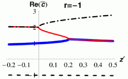
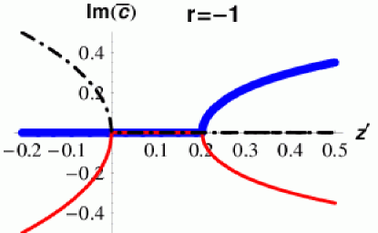
Figure 7: Real and imaginary parts of roots $\bar{c}$ for $r=-1$, plotted against $z^{\prime}$. The variable $z^{\prime}$ is chosen so that the continuum gap occurs at $z^{\prime}=1$. The thickest solid curve (blue) shows the root of interest, which has $\bar{c}=1$ at $z^{\prime}=0$. It joins with the thinner solid curve (red) at the start of the gap, and for large $z^{\prime}$ these form a complex conjugate pair. The other roots are shown as dashed and dot-dashed.

As one moves away from the continuum limit, the discretization errors in the gap become more pronounced. Figure 8 shows the roots for $r=-10$, for which the gap is $\approx 2\%$ of the continuum result. By contrast, fig. 8 ($r=-1/9$) shows the gap moving towards its continuum value as one reduces the discretization errors. Very close to the continuum ($r=-1/99$), the gap is almost unity, and the roots track those for $a=0$ except close to the gap, as illustrated in fig. 9.

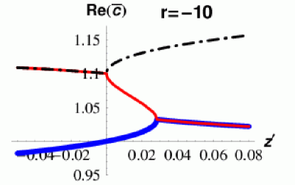
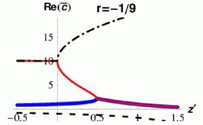
Figure 8: Real parts of roots for (a) $r=-10$ and (b) $r=-1/9$. Notation is as in fig. 7. The vertical scale is chosen to magnify the region of interest, so that not all roots appear in (a).

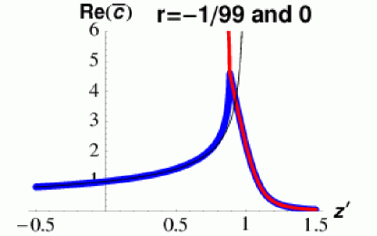
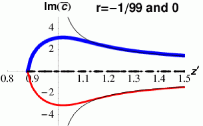
Figure 9: Real and imaginary parts of roots for $r=-1/99$ (with notation as in fig. 7, except not all roots appear given the vertical scales) compared to those in the continuum limit, $r=0$ (shown as a thin solid [black] line). Note that the horizontal scales differ in the two plots.

I next show how the gap depends on the pion mass-squared at fixed $a$. In order to facilitate comparison with the results of Ref. DD , I plot the gap for $Q_{m}$ (which is called $\mu$ in Ref. DD , but which I call $\mu_{Q}$ here to avoid confusion with the twisted mass). More precisely, I plot, in fig. 10, $2B_{0}\mu_{Q}/|w_{8}|=2B_{0}\sqrt{\bar{\alpha}/w_{8}^{2}}$ versus $m_{\pi}^{2}/|w_{8}|$. Dividing by $|w_{8}|$ gives dimensionless quantities. If $|r_{68}|\ll 1$, the $x$-axis gives the pion mass-squared in units of the Aoki-phase half-length. The quantities are such that, in the continuum limit, the result is a straight line with unit slope.

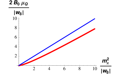
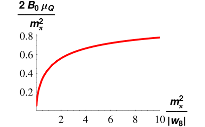
Figure 10: Results for the spectral gap of $Q_{m}$, $\mu_{Q}$, plotted against $m_{\pi}^{2}/|w_{8}|$. (a) Gap in dimensionless units, $2B_{0}\mu_{Q}/|w_{8}|$ (thick [red] curve) and result in continuum limit (thin [blue] curve); (b) Ratio of gap to $m_{\pi}^{2}/(2B_{0})$, which is unity in continuum limit. Results are for $w_{8}<0$.

The predicted gap is smaller than the continuum expectation. To bring this out, I show in fig. 10 the ratio of the gap to the continuum result, $m_{\pi}^{2}/(2B_{0})$. This approaches unity for $m_{\pi}^{2}/|w_{8}|\gg 1$, but the discretization errors reduce it significantly as one approaches the Aoki-phase end point. The analytic form of the result as $m_{\pi}^{2}\to 0$ is

$$\frac{2B_{0}\mu_{Q}}{m_{\pi}^{2}}=\frac{2B_{0}\sqrt{\bar{\alpha}}}{m_{\pi}^{2}}=\left(\frac{2}{3}\right)^{3/2}\sqrt{\frac{m_{\pi}^{2}}{|w_{8}|}}\,.$$ (61)

Note that the vanishing of the gap at the end point does not imply that the ratio of fig. 10 must vanish too. It would be sufficient if the ratio tended to a finite constant as $m_{\pi}^{2}\to 0$. Thus discretization errors lead to an additional reduction in the gap, which makes simulations less “safe” in the sense of Ref. DD . The square-root behavior is related to the mean-field exponents that apply at LO. In fact, if one approaches too close to the end point, higher order terms in $\chi$PT become important, and the exponents are corrected Aoki03 ; observations .

The method also yields the discretization errors in the integrated spectral density. I show the impact of these errors for the standard values of $r$ in fig. 11. The units of $N_{R}(\alpha)$ are such that the continuum result (55) is

$$\frac{\pi}{B_{0}f^{2}m_{\rm eff}}\times N_{R}(\alpha)=2\sqrt{\alpha/m_{\rm eff}-1}\,.$$ (62)

The figure shows what happens if $m$ is held fixed and the lattice spacing reduced. If $|w_{6}|\ll|w_{8}|$, then far above the gap the integrated density is unaffected by discretization errors, while there are significant downward shifts at the low end of the spectrum. In other words, aside from the smallest eigenvalues, say those with $\alpha<3m^{2}$, the spectrum is that of the continuum using the mass $m$. Note that this is not the quark mass which vanishes at the Aoki-phase end point (where $m_{\pi}\to 0$). It is the so-called PCAC mass, which vanishes instead in the center of the Aoki phase. The effect of a non-vanishing $w_{6}$ is essentially to shift the spectrum as a whole by an amount of $O(a^{2})$.

Figure 11: Results for integrated spectral density $N_{R}(\alpha)$. I plot $[\pi/(B_{0}f^{2}m_{\rm eff})]\times N_{R}(\alpha)$ versus $\alpha/m_{\rm eff}^{2}$, where $m_{\rm eff}=m+w_{6}/B_{0}=\widehat{m}^{\rm eff}/(2B_{0})$. Moving from top to bottom, results are for $r=-10$ (magenta), $-1$ (blue), $-1/9$ (red), $-1/99$ (green) and $r=0$ (black). The latter is the continuum result if $w_{6}=0$. Note that the upper two curves do have a gap (i.e. $N_{R}(\alpha)$ only becomes non-zero starting at a non-zero value of $\alpha$), but this is not visible in the figure.

I now explain the failure of the method for $w_{8}>0$. It turns out that the nature of the failure depends on the sign of $\widehat{m}^{\rm eff}=\widehat{m}+2w_{6}$. As can be seen from fig. 6, the boundary between positive and negative $\widehat{m}^{\rm eff}$ is also the line along which $r=1$.

I first consider $\widehat{m}^{\rm eff}\geq 0$ which, given that $w_{8}>0$, implies that $0<r\leq 1$. For $|r_{68}|<1$ this corresponds to the first-order scenario. I show the real part of the roots for a representative choice, $r=1/3$, in fig. 12. This corresponds to $r^{\prime}=2$ if $r_{68}=0$, i.e. discretization errors and the quark mass contribute about equally to the pion mass. The key point to note is that the root of interest, which passes through $\bar{c}=1$ at $z^{\prime}=0$, is real for all real choices of $z^{\prime}$. This remains true throughout the range $0<r<1$.

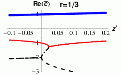
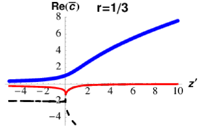
Figure 12: Real part of roots for $r=1/3$, for two choices of scale of $z^{\prime}$. The root of interest is shown by the thick (blue) solid line.

This result implies that there is no discontinuity in the potential, and, using eq. (50), that the integrated spectral density vanishes at LO. This is a peculiar result, particularly because, by sending $w_{6},w_{8}\to 0$ (implying $r\to 0^{+}$) one can approach arbitrarily close to the continuum, where the method works and one obtains a non-vanishing spectral density. Mathematically, what happens is as follows. Although the root of interest does not join with others for real $z^{\prime}$, it does so at a pair of complex conjugate values. Thus there are two cuts in the complex plane, as illustrated in fig. 13. As $r\to 0^{+}$, the two cuts come together at $z^{\prime}=1$, leading to a single cut on the real axis, given by the continuum result eq. (54). As $r$ varies between $0$ and $1$, the ends of the cuts follow the paths in the complex plane sketched in fig. 13. They come together again when $r=1$, leading to a cut along the negative $z^{\prime}$ real axis starting at $z^{\prime}=-1$.

Figure 13: Analytic structure of ${\cal V}^{\rm aux}_{\mu}(z^{\prime})$ for $w_{8}>0$ and $\widehat{m}^{\rm eff}>0$, corresponding to $0<r<1$. The cuts (thick [red] lines) are shown for the example of $r=0.1$. As usual, the position of the cuts is a convention, while their end points are fixed. The trajectory of the end points as $r$ changes is shown by the (blue) dots. The values of $r$ chosen are $0$, $0.01$, $0.1$, $1/3$, $1/2$, $2/3$, $0.9$, $0.99$ and $1.0$. Note the symmetry under $r\to 1-r$, $Re[z^{\prime}]\to-Re[z^{\prime}]$.

The implication of these results is that for $w_{8}>0$ and $\widehat{m}^{\rm eff}\geq 0$ the analytic structure of the root of interest, which is inherited by the potential ${\cal V}^{\rm aux}_{\rm min}$, differs from that of $F(z)$. Recall that the latter has, by construction, a cut only along the positive real axis, starting at $\bar{\alpha}>0$. Thus the result derived above relating $F$ to ${\cal V}^{\rm aux}_{\rm min}$, eq. (49), fails. The conclusion I draw is that the LO approximation is inconsistent for $F(z)$ if $w_{8}>0$, and higher order terms are needed, a possibility already discussed following eq.(33). An alternative is that the gap vanishes, so that the primary method is inapplicable, but this is implausible as it does not match onto the continuum result as $a\to 0$.

The method fails for essentially the same reason when $w_{8}>0$ and $\widehat{m}^{\rm eff}<0$. This corresponds to $1<r<\infty$, and, in fig. 6, is the region below the horizontal $r=1$ line. The generic behavior of the roots is illustrated by the example of $r=2$, shown in fig. 14. Because $\widehat{m}^{\rm eff}<0$ the root which minimizes the potential for real $\mu$ is that for which $\bar{c}=-1$ at $z^{\prime}=0$. For $1<r<\infty$, this root does not connect with any others for real $z^{\prime}$. The situation is very similar to that for $\widehat{m}^{\rm eff}>0$, namely there are two cuts in the complex plane. As before, since this analytic structure differs from that of $F(z)$, it must be that the approximations leading to the relation (49) break down.

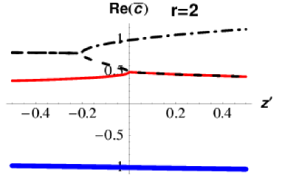
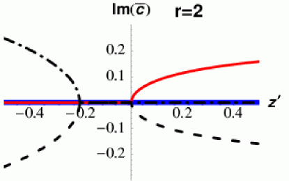
Figure 14: Real and imaginary parts of roots for $r=2$. The root of interest is that shown by the thick (blue) line.

Despite the failure of the method for $w_{8}>0$, there is no reason to doubt the validity of results obtained for $w_{8}<0$. These results provide a self-consistent solution for $F(z)$ and thus for the resolvent $R_{R}(z)$. What I mean by this is that the series for $R_{R}(z)$, evaluated term by term at LO, and summed, gives an analytic function with a cut only on the real $z$ axis, and no other singularities. This follows from the properties of the roots of the quartic, but, to be sure, I have checked this result numerically by verifying the dispersion relation eq. (10) for real $z<\bar{\alpha}$. I stress that the self-consistency of the LO result does not imply that there are no higher order corrections to $\rho_{R}(\alpha)$ and $R_{R}(z)$.

VI Discussion and Outlook

In this paper I have attempted to generalize the methods developed in the continuum for calculating the spectral density of $-i{\rm D}\!\!\!\!/\,$ to the operator of interest for the lattice theory, $Q_{m}$. The generalization necessary for the inclusion of discretization errors turned out, at least in the approaches I have followed, to be rather involved and only partly successful at leading-order.

Nevertheless, the success of the method for $w_{8}<0$ leads to a result which is relevant for numerical simulations, namely the reduction in the spectral gap of $Q_{m}$ compared to the continuum expectation. Since this likely applies only for the scenario in which discretization errors lead to an Aoki phase, it is probably not directly applicable to the numerical results for the gap obtained in Ref. DD . These are obtained with the Wilson gauge and fermion actions, for which one is apparently in the first-order scenario.

The result may be relevant, however, for simulations that are presently underway using improved Wilson fermions and/or improved gauge actions, for which the phase structure has not been established. With this in mind, I briefly discuss the way in which the discretization errors in the gap might best be seen. Looking at fig. 10, one sees that, for $m_{\pi}^{2}/|w_{8}|\mathrel{\hbox to0.0pt{\lower 3.0pt\hbox{$\mathchar 536\relax$}\hss}\raise 2.0pt\hbox{$\mathchar 318\relax$}}2$ a linear fit of $\mu_{Q}$ to $m_{\pi}^{2}$ (or, at this order, equivalently to $m$) would work reasonably well, but there would be a non-zero, negative intercept, and the slope would be smaller than the continuum expectation. Significant curvature should appear below this point. If one were in the Aoki-phase scenario with $w_{6}\approx 0$ and $|w_{8}|$ having a numerical value close to that which explains the first-order transition observed with Wilson gauge and fermion actions, i.e. if $w_{8}=-a^{2}\Lambda^{4}$ with $\Lambda\approx 700MeV$, then this “critical mass” is $m_{\pi}=250$ and $150\;$MeV at $a=0.1$ and $0.06\;$fm, respectively. Of course, if $\Lambda$ were reduced by a factor of 2, as might be achieved by using alternate actions, these values for $m_{\pi}$ would be reduced by a factor of four.

It is important to note that, since the discretization effects discussed here are of $O(a^{2})$, there is no a priori reason to expect them to be smaller for improved quark actions. One must simply investigate the issue numerically.

On the theoretical side, the failure of the primary method at LO for $w_{8}>0$ is puzzling. One can imagine working at arbitrarily small $a$ and $m$ where one would expect the corrections to the LO form to become arbitrarily small, and yet, apparently, they must be able to lead to a significant change in the analytic structure of the resolvent $R_{R}(\alpha)$. In an attempt to understand this puzzle I have repeated the calculation using a second method, and, although some new features appear, they do not appear to provide a solution for general values of the low-energy constants (and in particular for $w_{6}\approx w_{7}\approx 0$).

Despite this puzzle, I stress again that the result for $w_{8}<0$ provides a self-consistent solution for $R_{R}(\alpha)$, and I see no reason to doubt this result.

Beyond the task of resolving the above-mentioned puzzle, there are a number of directions in which it would be interesting to pursue this work. It could be applied for non-zero twisted sea-quark mass, although this is perhaps more of theoretical than practical interest as the gap is known to be bounded by the twisted mass. Of more practical interest would be to determine the impact of working at finite volume. I expect the corrections to the results for the spectral density to be exponentially suppressed until one enters the $\epsilon$-regime. As noted in the introduction, however, fluctuations in the gap have been observed to fall as inverse powers of $V$, and it would be interesting to see whether the effective theory can reproduce this behavior.

Appendix A Derivation of key result

In this appendix I demonstrate the result in eq. (34), which I repeat here for clarity:

$$2(n-1)!\langle P_{R}^{n}\rangle_{PQ,LO}=\langle(P_{R,12}+P_{R,21})^{n}\rangle_{CONN,LO}\,,\qquad(n\geq 1)\,.$$ (63)

As noted in the text, this result is trivial if $n$ is odd, so I assume that $n$ is even in the following. Recall that both correlators are to be calculated using the auxiliary chiral potential ${\cal V}^{\rm aux}_{\chi}$ of eq. (28), in which there are only single-supertrace operators.

The demonstration is based on the following results.

1. Only charged pion propagators appear in $\langle(P_{R,12}+P_{R,21})^{n}\rangle_{CONN,LO}$ and $\langle P_{R}^{n}\rangle_{PQ,LO}$.

   Charged here means being flavor off-diagonal, e.g. “12” or “35”, while neutral means flavor diagonal: “11”, “22” …. The argument goes as follows. Tree-level diagrams can always be divided into two pieces by cutting any propagator. Assume that there is a neutral pion propagator and cut it. Since the operators $P_{R}$ are all charged, there must be an even number in each of the two resulting pieces to add up to an overall neutral combination. But an even number of $P_{R}$’s can, together, produce only an even number of pions, which, through interactions, can only change to an even number of pions. Thus one reaches a contradiction.

   In fact, for $\langle P_{R}^{n}\rangle_{PQ,LO}$ the argument is more simple: the only set of pseudoscalar operators which are neutral is the whole set, but that leaves no operators for the other piece of the diagram.

2. For each pionic diagram contributing to the correlators of interest, one can unambiguously associate a finite number of planar quark-flow diagrams.

   This holds true as long as one does not have neutral pion propagators, as is the case here given observation (I). To obtain the quark-flow diagram one simply follows the flavor indices, connecting them into a single “trace” at each vertex and at each pseudoscalar operator. The flows are directed, with arrows indicating the flow of fermion number. Note that I do not distinguish between diagrams in which the flavor labels are permuted: these are all lumped into a single quark-flow “skeleton”, with the counting of possible attachments of flavor labels to be done below.

   For each pion-level diagram there are, in general, multiple quark-flow diagrams, corresponding to different orderings of the contractions between the $P_{R}$. For example, the pion-level diagram of fig. 2c leads to the three quark-flow diagrams of fig. 3b-d. I have drawn the diagrams in fig. 3 to be planar, in the sense that no quark-lines cross. This is their canonical form, for then the quark-line runs around the outside of the diagram, and the connection of flavor indices is transparent. That it is always possible to draw the quark-flow diagrams in this way is property of tree-level diagrams, following from the fact, noted above, that tree diagrams fall into two pieces if one cuts any propagator. Thus one can cut all propagators, make each vertex and insertion of $P_{R}$ planar, and then glue the propagators back together starting from an arbitrary point in the diagram, resulting in an overall planar diagram. The key point is that the vertices and insertions can be treated independently.

3. All contributions to $\langle P_{R}^{n}\rangle_{PQ,LO}$ contain a single quark-line in the corresponding quark-flow diagrams.

   For each quark-line in the diagram, all of which are necessarily closed, the total “charge” of the $P_{R}$ attached to it must vanish. Given the charges in $\langle P_{R}^{n}\rangle_{PQ}$ (see eq. 13), this is only possible if all the $P_{R}$ are attached to a quark-line, so there can only be one such line. Examples are shown in fig. 3. This result implies the (rather obvious) fact that there are no disconnected contributions to $\langle P_{R}^{n}\rangle_{PQ,LO}$.

4. All contributions to $\langle(P_{R,12}+P_{R,21})^{n}\rangle_{CONN,LO}$ contain a single quark-line in the corresponding quark-flow diagrams.

   This result relies on the facts that ${\cal V}^{\rm aux}_{\chi}$ contains only single-supertrace operators and that there are no neutral propagators [observation (I)]. These facts imply that there is no way for a quark-line to “close off” within a vertex or a propagator. (Examples of how this is possible with two-supertrace operators are given in fig. 4a-b.) Thus, if there is more than one quark-line, the pion diagram must fall into as many pion-disconnected pieces as there are quark-lines. This cannot happen, by definition, if the diagram is connected at the pion-level.

   Note that this result fails beyond LO. A one-loop example of a contribution to $\langle(P_{R,12}+P_{R,21})^{4}\rangle_{CONN}$ which involves two quark-lines, and is thus absent in $\langle P_{R}^{4}\rangle_{PQ}$, is given in fig. 15.

   Figure 15: Example of quark-flow for a one-loop diagram involving two single-supertrace operators which cannot contribute to $\langle P_{R}^{4}\rangle_{PQ}$ but which does contribute to $\langle(P_{R,12}+P_{R,21})^{4}\rangle_{CONN}$.

5. The same planar quark-line diagrams contribute to $\langle(P_{R,12}+P_{R,21})^{n}\rangle_{CONN,LO}$ and $\langle P_{R}^{n}\rangle_{PQ,LO}$.

   Any pion-level diagram contributing to $\langle(P_{R,12}+P_{R,21})^{n}\rangle_{CONN,LO}$ can also contribute to $\langle P_{R}^{n}\rangle_{PQ,LO}$, and vice-versa, since the vertices and insertions of $P_{R}$ produce the same number of pions in both cases. Thus the pion-level diagrams are the same for both correlators.

   The remaining question is whether the quark-flow diagrams that contribute to a given pion-level diagram are the same for both correlators. That this is the case can be seen as follows. From (III) and (IV), all quark-line diagrams contributing to both correlators involve a single quark-line. Adding back in the flavor indices, these will alternate as $1212\dots 2$ in the unquenched correlator, and as $1234\dots(2n)$ in the PQ correlator, as illustrated in fig. 16. Simply by interchanging these flavor labels one interchanges legitimate quark-line diagrams in the two correlators. Thus if a quark-flow diagram is present in one correlator, it will be present in the other.

6. The relative contribution from each planar quark-flow diagram to $\langle(P_{R,12}+P_{R,21})^{n}\rangle_{CONN,LO}$ and $\langle P_{R}^{n}\rangle_{PQ,LO}$ is the relative contraction factor $2(n-1)!$.

   The contributions to both correlators have now been broken down to those from a sum over (the same) planar quark-line diagrams. These diagrams are nothing more than an explicit representation of all the ways the flavor indices are connected when the pion fields are contracted. Thus all flavor factors are accounted for explicitly. The other factors that contribute to the diagram are the propagators, the factors which result from expanding out $\Sigma$ and $\Sigma^{\dagger}$ to obtain the vertices and insertions, and the counting of contractions. Only the latter differ between PQ and unquenched correlators. The propagators are the same because all quark masses are the same, and the expansion of $\Sigma^{(\dagger)}$ leads to the same factors in both theories. Furthermore, the “internal” counting of contractions—how many ways the pion fields in the vertices can be contracted with each other to yield the given planar quark-flow diagram—are also common. The only part of the calculation which differs between the theories is the choice of contractions with the external $P_{R}$. In the unquenched correlator, there are $2\times n!$ ways of associating the $n$ operators $(P_{R,12}+P_{R,21})$ with the external insertions: $n!$ since each operator can be attached to each insertion point, and $2$ because, for each such attachment, one can globally interchange $P_{R,12}$ and $P_{R,21}$. By contrast there are only $n$ contractions in the PQ case, because cyclicity must be preserved. Thus the relative factor is $2(n-1)!$, as claimed.

In summary, by breaking the diagrams up into planar quark-flow parts, which are common to both PQ and unquenched correlators, the problem is reduced to counting contractions. The counting is the same for all planar quark-flow diagrams with a given value of $n$, and thus eq. (63) follows.

Figure 16: Examples of flavor labels for a planar quark-flow diagram contributing to fig. 2c for (a) $\langle(P_{R,12}+P_{R,21})^{6}\rangle_{CONN}$, and (b) $\langle P_{R}^{6}\rangle_{PQ}$.

Appendix B Calculation using alternate method

The aim of this appendix is to check the results, and to understand the limitations, of the primary method, by repeating the calculation using an alternate method, in which partial quenching is implemented using the replica trick.

The starting point is eq. (7), which shows that one can obtain the average of the positive and negative spectral densities by determining the discontinuity in the twisted valence condensate. To determine this condensate at LO using the replica trick one needs to minimize the potential of a theory with $N_{S}=2$ sea-quarks and $2N_{V}$ replica quarks. Note that this theory is unquenched, and so has a well-defined and bounded Hamiltonian. The use of $2N_{V}$ replica quarks, rather than $N_{V}$, is for later convenience. Having calculated the condensate at the minimum, one then sends $N_{V}\to 0$, giving the valence condensate, and finally analytically continues to complex $\mu$ to determine the discontinuity across the imaginary axis.

The LO chiral Lagrangian takes the same form as that in the PQ theory, eq. (20), except that $\Sigma\in SU(N_{S}+2N_{V})$ and supertraces are replaced by traces. The potential is thus

$$\frac{{\cal V}_{\chi}^{\rm rep}(\mu)}{f^{2}}=-\frac{\mathrm{Tr}\left(\chi^{\rm rep}_{+}\Sigma^{\dagger}+\Sigma\chi^{\rm rep}_{-}\right)}{4}-w_{6}\frac{\left[\mathrm{Tr}\left(\Sigma+\Sigma^{\dagger}\right)\right]^{2}}{16}-w_{7}\frac{\left[\mathrm{Tr}\left(\Sigma-\Sigma^{\dagger}\right)\right]^{2}}{16}-w_{8}\frac{\mathrm{Tr}\left(\Sigma^{2}+{\Sigma^{\dagger}}^{2}\right)}{16}\,.$$ (64)

The mass term takes the block form

$$\chi^{\rm rep}_{\pm}={\rm diag}(\underbrace{\widehat{m}}_{2\times 2{\rm\ sea\ block}},\underbrace{\widehat{m}\pm i\widehat{\mu}\tau_{3},\ \dots\ ,\widehat{m}\pm i\widehat{\mu}\tau_{3}}_{N_{V}\ 2\times 2{\rm\ blocks}})\,.$$ (65)

The twisted mass appears only in the replica parts of the mass matrix since we are interested in the spectral density of $Q_{m}$ for a sea sector with an untwisted mass. I recall that when using the replica trick one takes the LECs ($w_{6}$ etc.) to be independent of $N_{V}$.

I assume that the form of $\Sigma$ which minimizes the potential follows that of the mass matrix, i.e.

$$\Sigma={\rm diag}(\underbrace{1}_{2\times 2{\rm\ sea\ block}},\underbrace{e^{i\omega\tau_{3}},\ \dots\ ,e^{i\omega\tau_{3}}}_{N_{V}\ 2\times 2{\rm\ blocks}})\,.$$ (66)

This can be shown to lead to a local minimum under certain assumptions on the parameters, as I discuss at the end of the appendix. With the condensate given by (66) the potential becomes

$$\frac{{\cal V}_{\chi}^{\rm rep}(\mu)}{f^{2}} \!=\! -\widehat{m}(1\!+\!N_{V}\cos\omega)-\widehat{\mu}N_{V}\sin\omega-w_{6}(1\!+\!N_{V}\cos\omega)^{2}-\frac{w_{8}}{4}(1\!+\!N_{V}\cos 2\omega)$$ (67)

$$\!=\! {\rm constant}-N_{V}\left[\widehat{m}^{\rm eff}\cos\omega+\widehat{\mu}\sin\omega+\frac{w_{8}}{4}\cos 2\omega\right]-N_{V}^{2}w_{6}\cos^{2}\omega\,.$$ (68)

Note that the $w_{7}$ term does not contribute, and that the same combination $\widehat{m}^{\rm eff}=\widehat{m}+2w_{6}$ appears as in the main text. As $N_{V}\to 0$, the term quadratic in $N_{V}$ can be dropped, and the determination of the minimum is to be done using only the contribution linear in $N_{V}$. This contribution is exactly the auxiliary potential encountered in the primary method, eq. (56). Thus the required minimizations in the two methods are identical, and yield the same minimizing angle, $\bar{\omega}(\mu)$.

It remains to be shown that the results for the spectral density are also the same. In the replica method, the required condensate is, using eq. (22),

$$\langle\bar{q}_{V}\gamma_{5}\tau_{3}q_{V}\rangle_{LO}=2iB_{0}f^{2}\sin\bar{\omega}\,.$$ (69)

Since this is the condensate for one replica doublet (and not $N_{V}$ doublets), it has a non-vanishing limit as $N_{V}\to 0$. Thus the final result from the replica trick is, using eq. (7),

$${B_{0}f^{2}}\ {\rm Disc}\ [\sin\bar{\omega}]\bigg{|}_{\mu=i\lambda}=\pi\left[\rho_{Q}(\lambda)+\rho_{Q}(-\lambda)\right]\,.$$ (70)

Note that the spectral density $\rho_{Q}$ is renormalized, since it is determined from a renormalized condensate.

This result is equivalent to that from the primary method, eq. (50). To see this, one takes the derivative of the latter equation with respect to $\alpha$, and uses the fact that the derivative commutes with taking the discontinuity:

$$-2i\pi\rho_{R}(\alpha)=\frac{d}{d\alpha}\left\{{\rm Disc}\;[{\cal V}^{\rm aux}_{\rm min}(\mu^{2}=-z)]\bigg{|}_{z=\alpha}\right\}=-{\rm Disc}\;[\frac{d}{d\mu^{2}}{\cal V}^{\rm aux}_{\rm min}(\mu^{2}=-z)]\bigg{|}_{z=\alpha}\,.$$ (71)

Next, one notes that the spectral density of $Q_{m}^{2}$ can be related to that of $Q_{m}$,

$${2\sqrt{\alpha}}\;\rho_{R}(\alpha)={\rho_{Q}(\sqrt{\alpha})+\rho_{Q}(-\sqrt{\alpha})}\,,$$ (72)

as well as the fact that

$$2\mu\frac{d{\cal V}_{\rm min}^{\rm aux}}{d(\mu^{2})}=\frac{d{\cal V}_{\rm min}^{\rm aux}}{d\mu}=-2B_{0}f^{2}\sin\bar{\omega}(\mu)\,.$$ (73)

Substituting these results into eq. (71) and performing some simple manipulations gives eq. (70). The derivation also runs in the other direction: the result in the text can be obtained from (70) as long as the discontinuity in $\sin\bar{\omega}$ is integrable, which is the case here.

I now return to the question of whether the assumed form of the condensate, eq. (66), is correct. This brings up the general question of how to apply the replica trick in a context where the dependence on $N_{V}$ is not perturbative. It seems possible, for example, that, for a given choice of LECs $w_{6-8}$, there could be a non-trivial $N_{V}$ dependence of the phase structure, and thus a non-analytic dependence of the condensate on $N_{V}$. This issue deserves further study, which I have not attempted here. The only general comment I can make is that, if $w_{6}=w_{7}=0$, then, for $w_{8}>0$ (which is the case in which the primary method fails), it is plausible that the condensate takes the form (66) for all integer $N_{V}$ and $\mu$ real. This is because the mass term wants to align $\Sigma\propto\chi^{\rm rep}_{+}$, while the $w_{8}$ term is minimized when $\Sigma=\pm 1$. These competing “pulls” seem likely to lead to a condensate which lies on the shortest path between the two favored directions, which is eq. (66). Thus I do not expect that studying the phase structure will resolve the failures of the primary method in general.

A more modest goal is to show that the form (66) leads to a local minimum. It is straightforward to show that minimizing the restricted replica potential (68) does lead to an extremum in all directions of possible fluctuations. Thus the issue is whether it is a minimum in all directions. Choosing a basis in which there is no mixing, I find, in the replica limit, that the pion mass-squareds are:

$$M_{SS}^{2} = \widehat{m}^{\rm eff}+w_{8}\,,$$ (74)

$$M_{VV,n}^{2} = \bar{c}\left(\widehat{m}^{\rm eff}+\frac{\widehat{\mu}^{2}}{\widehat{m}^{\rm eff}+w_{8}\bar{c}}\right)+{w_{8}}\;(2\bar{c}^{2}-1)\,,$$ (75)

$$M_{VV,c}^{2} = M_{VV,n}^{2}+w_{8}\;(1-\bar{c}^{2})\,,$$ (76)

$$M_{VS,n}^{2} = M_{VV,n}^{2}+w_{7}\;(1-\bar{c})^{2}\,,$$ (77)

$$M_{VS,c}^{2} = \frac{M_{SS}^{2}+M_{VV,n}^{2}+w_{8}\;\bar{c}(1-\bar{c})}{2}\,.$$ (78)

Here $\bar{c}=\cos\bar{\omega}$, the subscripts “c” and “n” stand for charged and neutral, respectively, and the other subscripts indicate the sea and valence content of the “pions”. If any of these mass-squareds passes through zero and becomes negative, then the extremum is unstable to fluctuations in the corresponding directions. Note that the alternate method has more directions of fluctuation than appear in the primary method. Most notable are the “VS” directions—these introduce the LEC $w_{7}$ which does not enter in the analysis of the main text.

If the alternate method is to resolve the puzzle from the main text, it should do so for all choices of $w_{7}$, and so I begin with the simplest, $w_{7}=0$. In this case, however, the results of the primary method are reproduced (as long as $\widehat{m}^{\rm eff}>0$, an exception discussed below). In particular, if $w_{8}>0$ (and $\widehat{m}^{\rm eff}>0$), all pion mass-squareds are positive for all real (positive and negative) values of $\mu^{2}$, so that the choice (66) with $\omega=\bar{\omega}$ is a local minimum. If $w_{8}<0$, however, then $M_{VV,n}^{2}$ vanishes when $\mu^{2}=-\bar{\alpha}$. This signals a non-analyticity in $\bar{c}$, which is inherited by the valence condensate, and is identical to the condition for the gap discussed in the main text. Thus the puzzle is not resolved for these parameter choices.

There are, however, two cases where the present analysis differs from that in the main text, both involving instabilities in which the mixed pions composed of valence and sea-quarks have vanishing masses. The most straightforward follows from eq. (77): as $\mu^{2}$ becomes more negative $M_{VS,n}^{2}$ can pass through zero and become negative if $w_{7}$ is sufficiently negative. It turns out that $w_{7}$ should not be too negative, however, because then $M_{VS,n}^{2}$ also changes sign as $\mu^{2}$ becomes more positive. Nevertheless, the conclusion is that there is a range of negative $w_{7}$ which could lead to the expected analytic structure.

The other possibility is more complicated. It occurs when $\widehat{m}^{\rm eff}<0$, i.e when $w_{6}$ is sufficiently negative ($2w_{6}<-\widehat{m}$) that the mass in the effective potential is negative even though $\widehat{m}$ itself is positive. Note that in this region one must have $w_{8}>|\widehat{m}^{\rm eff}|$, as shown in fig. 6. As noted in the main text, if $\widehat{m}^{\rm eff}<0$, the minimum of auxiliary potential (or equivalently of ${\cal V}_{\chi}^{\rm rep}$ for $N_{V}\to 0$) lies at $\bar{c}=-1$ if $\mu=0$. The mass formulae given above still hold, but now the contribution to $M_{VS,c}^{2}$ proportional to $w_{8}\bar{c}(1-\bar{c})$ is negative. This has the effect that $M_{VS,c}^{2}$ vanishes exactly at $\mu^{2}=0$, and becomes negative for $\mu^{2}<0$, for all allowed $w_{8}$. The vanishing at $\mu^{2}=0$ can be understood from the viewpoint of the original replica potential, ${\cal V}_{\chi}^{\rm rep}$. If $\bar{c}=-1$, then the condensate takes the form

$$\langle\Sigma\rangle={\rm diag}(1,-1,\dots,-1)\,.$$ (79)

This breaks the $SU(2+2N_{V})$ vector symmetry of the theory that is exact when $\mu=0$. Thus, as in the Aoki-phase analysis, there are exact Goldstone bosons, here the $VS$ pions. This symmetry breaking arises because, for $w_{6}$ negative, the $w_{6}$ term favors a condensate rotated away from $\pm 1$.

This instability seems to imply a discontinuity in $\bar{c}$, and thus in the valence condensate, beginning at $-\mu^{2}=0$. This would correspond to the gap vanishing. If correct, this could explain the failure of the primary method, which, unlike the present approach, relies on the gap being non-zero. Note that one cannot reach the continuum limit in the region of parameters where this possible resolution applies ($\widehat{m}^{\rm eff}<0$, $w_{8}>|\widehat{m}^{\rm eff}|$), so there is no contradiction with the result that the gap is non-vanishing in the continuum.

I have not pursued this analysis further, since the possible resolutions of the problem for $w_{8}>0$ are not general. In particular, they do not apply if $\widehat{m}\mathrel{\hbox to0.0pt{\lower 3.0pt\hbox{$\mathchar 536\relax$}\hss}\raise 2.0pt\hbox{$\mathchar 318\relax$}}w_{8}\mathrel{\hbox to0.0pt{\lower 3.0pt\hbox{$\mathchar 536\relax$}\hss}\raise 2.0pt\hbox{$\mathchar 318\relax$}}|2w_{6}|$, which is the region through which one likely approaches the continuum limit if one is in the first order scenario.

References

- (1) M. Lüscher, PoS LAT2005, 002 (2005) [arXiv:hep-lat/0509152].
- (2) M. Lüscher, JHEP 0305, 052 (2003) [arXiv:hep-lat/0304007].
- (3) M. Hasenbusch, Phys. Lett. B 519, 177 (2001) [arXiv:hep-lat/0107019].
- (4) C. Urbach, K. Jansen, A. Shindler and U. Wenger, Comput. Phys. Commun. 174, 87 (2006) [arXiv:hep-lat/0506011].
- (5) L. Del Debbio, L. Giusti, M. Lüscher, R. Petronzio and N. Tantalo, JHEP 0602, 011 (2006) [arXiv:hep-lat/0512021].
- (6) M. Creutz, arXiv:hep-ph/9608216.
- (7) S. R. Sharpe and R. L. Singleton, Phys. Rev. D 58, 074501 (1998) [arXiv:hep-lat/9804028].
- (8) S. Aoki, Phys. Rev. D 30, 2653 (1984); Phys. Rev. Lett. 57, 3136 (1986); Prog. Theor. Phys. 122, 179 (1996).
-
(9)
F. Farchioni et al.,
Eur. Phys. J. C 39, 421 (2005)
[arXiv:hep-lat/0406039];
F. Farchioni et al., Eur. Phys. J. C 42, 73 (2005) [arXiv:hep-lat/0410031];
F. Farchioni et al., arXiv:hep-lat/0512017;
F. Farchioni et al., Phys. Lett. B 624, 324 (2005) [arXiv:hep-lat/0506025]. - (10) T. Banks and A. Casher, Nucl. Phys. B 169, 103 (1980).
- (11) G. Rupak and N. Shoresh, Phys. Rev. D 66, 054503 (2002) [arXiv:hep-lat/0201019].
- (12) O. Bär, G. Rupak and N. Shoresh, Phys. Rev. D 70, 034508 (2004) [arXiv:hep-lat/0306021].
- (13) J. C. Osborn, D. Toublan and J. J. M. Verbaarschot, Nucl. Phys. B 540, 317 (1999) [arXiv:hep-th/9806110].
- (14) P. H. Damgaard, J. C. Osborn, D. Toublan and J. J. M. Verbaarschot, Nucl. Phys. B 547, 305 (1999) [arXiv:hep-th/9811212].
- (15) C. W. Bernard and M. F. L. Golterman, Phys. Rev. D 49, 486 (1994) [arXiv:hep-lat/9306005].
- (16) A. V. Smilga and J. Stern, Phys. Lett. B 318, 531 (1993).
- (17) M. Golterman, Y. Shamir and B. Svetitsky, Phys. Rev. D 71, 071502 (2005) [arXiv:hep-lat/0407021]; ibid D 72, 034501 (2005) [arXiv:hep-lat/0503037].
- (18) G. Münster, JHEP 0409, 035 (2004) [arXiv:hep-lat/0407006].
- (19) L. Scorzato, Eur. Phys. J. C 37, 445 (2004) [arXiv:hep-lat/0407023].
- (20) S. R. Sharpe and J. M. S. Wu, Phys. Rev. D 70, 094029 (2004) [arXiv:hep-lat/0407025].
- (21) S. Aoki and O. Bär, Phys. Rev. D 70, 116011 (2004) [arXiv:hep-lat/0409006].
- (22) M. Golterman, S. R. Sharpe and R. L. . Singleton, Phys. Rev. D 71, 094503 (2005) [arXiv:hep-lat/0501015].
-
(23)
P. H. Damgaard,
Phys. Lett. B 476, 465 (2000)
[arXiv:hep-lat/0001002];
P. H. Damgaard and K. Splittorff, Phys. Rev. D 62, 054509 (2000) [arXiv:hep-lat/0003017] - (24) S. R. Sharpe and N. Shoresh, Phys. Rev. D 64, 114510 (2001) [arXiv:hep-lat/0108003].
- (25) S. R. Sharpe and J. M. S. Wu, Phys. Rev. D 71, 074501 (2005) [arXiv:hep-lat/0411021].
- (26) S. R. Sharpe and N. Shoresh, Phys. Rev. D 62, 094503 (2000) [arXiv:hep-lat/0006017].
- (27) S. R. Sharpe and R. S. Van de Water, Phys. Rev. D 69, 054027 (2004) [arXiv:hep-lat/0310012].
- (28) S. Aoki and O. Bar, PoS LAT2005, 046 (2006) [arXiv:hep-lat/0509002]; arXiv:hep-lat/0604018.
- (29) S. R. Sharpe, Phys. Rev. D 72, 074510 (2005) [arXiv:hep-lat/0509009].
- (30) S. Aoki, Phys. Rev. D 68, 054508 (2003) [arXiv:hep-lat/0306027].