Phase Structure of -Polyakov-Loop Models
Abstract
We study effective lattice actions describing the Polyakov loop dynamics originating from finite-temperature Yang-Mills theory. Starting with a strong-coupling expansion the effective action is obtained as a series of -invariant operators involving higher and higher powers of the Polyakov loop, each with its own coupling. Truncating to a subclass with two couplings we perform a detailed analysis of the statistical mechanics involved. To this end we employ a modified mean field approximation and Monte Carlo simulations based on a novel cluster algorithm. We find excellent agreement of both approaches concerning the phase structure of the theories. The phase diagram exhibits both first and second order transitions between symmetric, ferromagnetic and anti-ferromagnetic phases with phase boundaries merging at three tricritical points. The critical exponents and at the continuous transition between symmetric and anti-ferromagnetic phases are the same as for the 3-state Potts model.
pacs:
02.50.Ng, 05.50.+q, 11.10.Wx, 11.15.Ha, 12.40.Ee, 75.10.Hk, 75.40.Mg, 75.50.EeI Introduction
In two seminal papers Svetitsky and Yaffe have tentatively linked the finite-temperature phase transitions in ‘hot’ gauge theories to the simpler order-disorder phase transitions of spin models Yaffe and Svetitsky (1982); Svetitsky and Yaffe (1982). In the general case their conjecture may be stated as follows: The effective theory describing finite-temperature Yang-Mills theory with gauge group in dimensions is a spin model in dimensions with a global symmetry group given by the centre of the gauge group. A somewhat stronger version of the conjecture can be formulated if the phase transitions in questions are of second order. In this case Yang-Mills theory and spin model fall into the same universality class and the critical exponents coincide. This has been convincingly demonstrated for Engels et al. (1990, 1992) in .
However, continuous phase transitions in hot gauge theories are not generic and hence the universality statement is almost empty – at least in 3+1 dimensions Holland et al. (2004a). On the other hand, the more general version of the statement has already been used by Svetitsky and Yaffe to argue that the phase transition for Yang-Mills theory must be first order for as there is no RG fixed point in this case. Since then this has been firmly established by a number of lattice calculations Celik et al. (1983); Kogut et al. (1983); Gottlieb et al. (1985); Brown et al. (1988); Fukugita et al. (1989); Alves et al. (1990).
The conjecture implies that the effective theories may be formulated as ‘Polyakov loop models’ Pisarski (2000, 2002); Dumitru et al. (2004). For this means that the macroscopic dynamical variables have to reflect the complete gauge invariant information contained in the (untraced) Polyakov loop, which in lattice notation is given by
| (1) |
This is a temporal holonomy winding around the compact Euclidean time direction of extent . For gauge groups with nontrivial centre the traced Polyakov loop,
| (2) |
with the trace being taken in the defining representation111We do not include a normalisation factor for the ease of later notation. serves as an order parameter for the deconfinement phase transition. The phase transition goes along with spontaneous breaking of the centre symmetry resulting from non-periodic gauge transformations under which
| (3) |
The deconfined broken-symmetry phase at sufficiently large Wilson coupling is characterised by (see Holland and Wiese (2000) for a review).
Recently it has been found that gauge groups with trivial centre may also lead to a deconfinement transition depending on the size of the gauge group Borgs and Seiler (1983); Holland et al. (2004b); Holland et al. (2003).
At this point the choice of dynamical variables needs to be addressed. Under periodic gauge transformations the holonomy (1) transforms as
| (4) |
which leaves its eigenvalues and, as a consequence, its trace (2) invariant. The eigenvalues are permuted arbitrarily by gauge transformations corresponding to Weyl reflections Ford et al. (1999). This invariance is taken into account by constructing symmetric polynomials in the eigenvalues. From unimodularity the product of the eigenvalues is and there are only independent polynomials, for example the traces for . These in turn are in one-to-one correspondence with the characters of the fundamental representations (see below). Hence, for (which is real) is sufficient while requires and , the latter being a linear combination of and . Only for traces of higher powers of are needed as independent dynamical variables Meisinger et al. (2002).
In two recent papers Dittmann et al. (2004); Heinzl et al. (2005) we have studied Polyakov loop models on the lattice for the simplest non-Abelian gauge group . The models have been derived using strong-coupling techniques at small Wilson coupling and a newly developed inverse Monte Carlo (IMC) method which works for arbitrary values of . The latter method allows for a mapping of Yang-Mills theory at a certain value of to any appropriately chosen Polyakov loop model of the form
| (5) |
where the summation is over nearest neighbours and group representations , . The group character is the trace of the Polyakov loop in representation ,
| (6) |
All characters are polynomials in the characters corresponding to the fundamental representations. For the simplest model is of Ising type,
| (7) |
as first suggested in Polonyi and Szlachanyi (1982) (see also Ogilvie (1984); Billo et al. (1996)).
The output of the IMC routines are the -dependent effective couplings . Even without particular knowledge of these one may study the models (5) in their own right as statistical field theories. The Svetitsky-Yaffe conjecture may then be utilised to deduce information about the Yang-Mills phase transition. For we have been able to show that the mean-field analysis of the effective models yields a surprisingly good agreement with the Monte Carlo analysis of both the model itself and the underlying Yang-Mills dynamics. It should be stressed at this point that the models (5) are not just simple scalar field theories with a linear target space as all characters (6) take values in a compact space parametrised by the fundamental characters. Hence, in the lattice path integral each lattice site is endowed with the reduced Haar measure on the gauge group rather than a Lebesgue measure.
This paper presents our first steps to generalise the results of Dittmann et al. (2004); Heinzl et al. (2005) to the gauge group . We label the characters by two integers and which count the numbers of fundamental and conjugate representations (‘quarks’ and ‘antiquarks’ in the flavour language) required to construct the representation . Equivalently, these integers characterise the horizontal extensions of Young tableaux (see Fig. 1).

Under the centre transformations the characters transform according to the rule
| (8) |
so that the most general centre-symmetric effective action with nearest-neighbour interaction may be written as
| (9) |
This coincides with the ansatz suggested by Dumitru et al. Dumitru et al. (2004). The first sum in the effective action consists of hopping terms involving monomials of the form or (and h.c.) while the second sum is a ‘potential’ term containing only powers (and h.c.) localised at single sites.
The remainder of the paper is organised as follows. In Section II we confirm the ansatz (9) by means of a strong coupling (small-) expansion for . For a restricted set of couplings (and hence representations) we investigate the resulting models by minimising the classical action (Section III) followed by an improved mean field analysis in Section IV. In agreement with the Svetitsky-Yaffe conjecture we find a first order phase transition from the symmetric to a ferromagnetic phase. Our improved mean field analysis already reveals an interesting phase structure with four different phases: two distinct ferromagnetic phases, one symmetric and one anti-ferromagnetic phase. Besides the first order transitions we detect second order transitions from the symmetric to an anti-ferromagnetic and to a ferromagnetic phase. The continuous transition from the symmetric to the anti-ferromagnetic phase is to be expected since the models reduce to the -state Potts model for Polyakov-loops having values in the centre of the gauge group. Section V contains the results of our extensive Monte Carlo simulations performed on a Linux cluster where we have implemented the powerful package jenLaTT. Similarly as for the mean field and numerical results are in surprisingly good agreement. This is presumably due to the existence of (three) tricritical points. Depending on the order of the transition we localise the critical lines with either a Metropolis, a multicanonical or a modified cluster algorithm. In addition we have checked that the critical exponents and at the second order transition to the anti-ferromagnetic phase agree with those of the -state Potts model in dimensions. Finally, in Section VI we wrap up with discussion and conclusions.
II Strong-Coupling Expansion
In this section we briefly recapitulate the strong-coupling (small-) expansion for the Wilson action at finite temperature Ogilvie (1984); Svetitsky (1986). It is known that the leading order result () stems from ladder diagrams that wind around the temporal lattice extension and corresponds to an Ising type model analogous to (7). By going beyond the leading order we will encounter higher group representations/characters and hence have an independent confirmation of the ansatz (9) for the effective action.
Our starting point is the standard Wilson action,
| (10) |
where the summation over plaquettes contains both temporal and spatial links. The effective action is introduced as usual by inserting an appropriate (group valued) delta function in the path integral,
| (11) |
While it is not known how to perform the final integration analytically for the full Wilson action one can straightforwardly integrate order by order in . Thus we expand the Boltzmann weight
| (12) |
and integrate separately over temporal and spatial links, . Adopting temporal gauge we set all temporal links equal to unity apart from the links in the first timeslice which according to (1) may be identified with the Polyakov loop. Integrating out all spatial link variables we obtain the partition function
| (13) |
where we have introduced the operators . The effective action may finally be written as
| (14) |
where the coefficients are related to the operators via the linked-cluster theorem. In the remainder of this section we are going to determine the explicit form of the effective operators .
We first rewrite the Wilson-Boltzmann weight (12) as
| (15) |
and expand the single-plaquette contribution in terms of characters,
| (16) |
with (see Fig. 1). All dependence now resides in the generalised Fourier coefficients which accordingly may be further expanded,
| (17) |
An explicit computation of the shows that these vanish whenever the representation labels become sufficiently large, namely if Buss (2004). This yields the important intermediate result that to any given order in the strong-coupling expansion only a finite number of characters contributes,
| (18) |
The integrations over the spatial links are standard group integrals which can be found in the texts Creutz (1983); Montvay and Münster (1994). The upshot is that only connected link arrangements (‘polymers’) wrapping around the temporal extent of the lattice yield nonvanishing contributions. The leading term is a ladder diagram consisting of plaquettes each of which contributes a factor of implying a total contribution of . The associated operator is explicitly found to be
| (19) |
A typical operator of order is given by
| (20) |
in terms of which the Wilson-Boltzmann weight (15) becomes
| (21) |
Expanding this to next-to-leading order () yields the simple expression
| (22) |
Note, however, that some care has to be taken in interpreting products such as which by (20) also contain disconnected pieces. Upon expanding the logarithm by means of the linked-cluster theorem we are led to keep only connected contributions of the form
| (23) |
Making use of the character reduction formula
| (24) |
products of characters at the same site may be reduced to single characters. As a consequence, the connected part of (22) takes the explicit form
| (25) |
For what follows it is useful to introduce the short-hand notation
| (26) |
with the obvious term-by-term identifications as compared to (25). Our conventions are such that all couplings in (25) and (26) are real functions of , the single leading one being (as noted already in Ogilvie (1984)) while the subleading ones are . It is straightforward to include higher-order terms the number of which increases rapidly. At order , for instance, there are already 11 terms so that we refrain from going beyond next-to-leading order in .
For later purposes it is useful to express the operators appearing in (26) in terms of the fundamental loops and . Octet and sextet characters ( and , respectively) are eliminated via the standard reduction identities
| (27) |
which are equivalent to the character relations (recall that )
| (28) |
Making use of the latter the different terms in (26) become
| (29) | ||||
| (30) | ||||
| (31) | ||||
| (32) | ||||
| (33) |
From these expressions it is obvious that each operator is manifestly real. Under charge conjugation , hence , whereupon all terms in are charge conjugation invariant as required Holland and Wiese (2000). Note that the orders included correspond to terms that are quadratic, cubic and quartic in and/or . Higher powers will arise upon taking into account higher representations. Thus, in this respect is somewhat singled out being of only cubic order. This will become important in a moment.
III Qualitative Classical Analysis
It has already been pointed out by Svetitsky and Yaffe Yaffe and Svetitsky (1982) that effective actions with centre symmetry are closely related to the 3-state Potts model which shows a first order phase transition from a symmetric to a ferromagnetic phase Jensen and Mouritsen (1979); Kogut and Sinclair (1982); Wu (1982). To make the relation manifest we restrict the Polyakov loop to the centre elements introduced in (8). Setting we find the general formula
| (34) |
where denotes the dimension of the representation ,
| (35) |
Applying this to the effective action in (26) we find, up to an additive constant,
| (36) |
with effective coupling
| (37) |
The action (36) is precisely the one of the 3-state Potts model Potts (1952); Wu (1982). We thus expect that our effective Polyakov loop models will have a phase structure generalising the one of the 3-state Potts model. The latter is known to have a ferromagnetic phase for large negative and an anti-ferromagnetic phase for large positive Janke and Villanova (1997); Gottlob and Hasenbusch (1994). As a preparation for the discussion of later sections it is hence useful to obtain some qualitative understanding of the phase structure of the Polyakov loop models viewed as generalisations of the 3-state Potts model. For the reason mentioned at the end of the previous section we choose as a minimal generalisation the following effective action,
| (38) |
which in terms of the fundamental loops may be written explicitly as
| (39) |
Note that there are also quadratic contributions stemming from . The action (39) is manifestly centre symmetric under .
It is important to realise that (39) differs from the standard lattice actions for scalar fields in several respects. First, the field is dimensionless, being the trace of a unitary matrix. This allows for the presence of cubic hopping terms connecting neighbouring sites. Even more important is the fact that the target space of is compact. Introducing the eigenvalues of via
| (40) |
and writing we find for the real and imaginary part of ,
| (41) | ||||
| (42) |
The target space of may then be sketched in the complex -plane (see Fig. 2). The boundary corresponds to the points with , the singular ‘corners’ being given by the three centre elements .
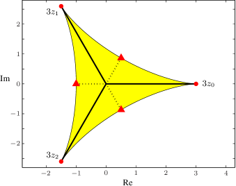
Let us try to get some first rough idea of the phase structure associated with the two-coupling model (39) in the - plane by looking at the extrema of the classical action. If we vary the couplings these will trace out a certain (possibly discontinuous) trajectory in the target space given by the triangle of Fig. 2.
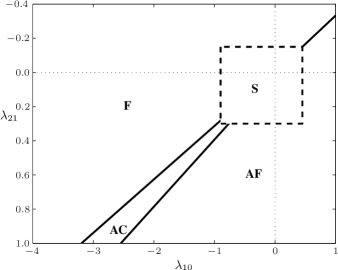
As we argued earlier, for centre-valued Polyakov loops the effective action (39) reduces to the action of the Potts model (36) with coupling . Thus we expect a ferromagnetic phase (F) for large negative and an anti-ferromagnetic phase (AF) for large and positive. In a region around the origin in the coupling plane entropy dominates energy and we cannot expect to actually obtain the correct phase-structure in this region by purely classical reasoning based on minimising the energy. Qualitatively we expect a symmetric phase in a neighbourhood of the origin. This is represented schematically in Fig. 3 by the central rectangle.
In order to study the ordered phases (in particular AF) we divide the lattice in two sub-lattices (denoted ‘even’ and ‘odd’) where the Polyakov loop takes values and , respectively. Two nearest neighbours belong to different sub-lattices. The absolute minima of the classical action
| (43) |
will then be located at certain values and of the Polyakov loop which are identified with its ‘expectation values’. We trust this reasoning as long as we are sufficiently far from the origin of the coupling plane i.e. from the disordered, entropy-dominated phase.
Any ferromagnetic ordering will be characterised by a minimum with while in an anti-ferromagnetic phase . Quite interestingly we find two distinct ferromagnetic phases, one for which the Polyakov loop is near a centre element or in the vicinity of and a different ferromagnetic phase with taking values near the intermediate points marked by triangles in Fig. 2. We call this an anti-centre phase (AC). We expect a phase transition line separating the ferromagnetic and anti-ferromagnetic phases at vanishing Potts-coupling . The resulting qualitative phase diagram is depicted in Fig. 3.
To discuss the ferromagnetic phases it suffices to minimize the action (43) with , in which case
| (44) |
This can be done analytically. To localise the anti-ferromagnetic phase we have calculated the absolute minima of (43) on the target space depicted in Fig. 2 numerically. The combined analytical and numerical results are summarised as follows. For negative we have a transition
| (45) |
while for positive there is a richer structure,
| (46) |
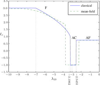
The behaviour of a suitably projected order parameter (the precise definition of which will only be needed later on) for positive is shown in Fig. 4. Upon inspection one notes that for sufficiently negative the system starts out with the Polyakov loop at a centre element. Increasing beyond the order parameter drops monotonically until, at a critical coupling , there is a jump to the AC phase with near a anti-centre element. The jump of is due to a centre-transformation and does not imply that the Polyakov loop itself jumps. Indeed, changes smoothly and arrives at an anti-center element for . The system stays there until , where it jumps again, this time to the AF phase. As expected, we see no symmetric phase in a purely classical analysis. Actually, for there is just no symmetric phase.
IV Mean field approximation
The next step of refinement to be presented in this section is a mean field (MF) analysis of the effective action (39). This will serve as a basis for a comparison with results from direct Monte Carlo simulations to be discussed later on. Due to the peculiarities of the model as compared to standard scalar field theories the application of the MF approximation is not entirely straightforward. For the benefit of the reader we will set the stage by giving a brief outline of the necessary modifications. For further details the reader is referred to our earlier paper Heinzl et al. (2005). To keep the discussion sufficiently general we will first treat the effective action (26) with five couplings focussing on simpler examples later on.
We are interested in expectation values which are computed by evaluating integrals of the form
| (47) |
which apparently extend over the whole group manifold employing the Haar measure . However, due to the gauge invariance of both action and measure the integrals can be reduced to the coset space of conjugacy classes which we (somewhat symbolically) denote by . Hence we integrate with the reduced Haar measure by replacing
| (48) |
Thus, (47) is equivalent to
| (49) |
The probability measure is characterized as the unique solution to the variational problem
| (50) |
The expectation value on the left-hand side has to be taken with respect to the integration measure with denoting the probability density of . From this point of view the MF approximation is nothing else but the restriction of the permissible densities to product form,
| (51) |
Expectation values can now be simply computed site by site via factorisation,
| (52) |
Our goal is to compute the effective potential as function of the mean characters . For that purpose we solve the variational problem (50) on the space of product measures with fixed expectation values of the characters. This is done by introducing appropriate Lagrange multipliers . For ferromagnetic systems one may assume that the weight functions at each site are identical, . This assumption corresponds to a translationally invariant ground state. According to the discussion of the previous section we expect anti-ferromagnetic phases and hence we must refine our choice for . We therefore introduce different weight functions on the even and odd sub-lattices, respectively,
| (53) |
defining the sign of a lattice point as
| (54) |
As a consequence, expectation values of characters will subsequently have two values depending on the sub-lattice where they are evaluated,
| (55) |
The sources are taken constant as well when restricted to the even and odd sub-lattices, or , respectively. Like the characters the sources are complex.
The action (21) couples only nearest-neighbour sites so that its expectation value entering (50) may be written as
| (56) |
with denoting the lattice volume in spatial dimensions. The logarithm in (50) decomposes as
| (57) |
It is convenient to drop the common volume factor and consider densities instead. The variation of (50) finally yields the weight function for the even sub-lattice,
| (58) |
and a completely analogous expression for the odd sub-lattice. Here we have introduced as a short-hand for and the single-site partition function
| (59) |
The sources are eliminated by inverting the relations
| (60) |
to be evaluated separately on both sublattices. The Schwinger function is defined as usual,
| (61) |
Introducing the Legendre transform of (61) according to
| (62) |
the solution of (50) is finally obtained as the MF potential (density) as a function of even and odd mean fields,
| (63) |
From this expression one can easily derive relations between the sources and mean characters . For instance, by varying with respect to we obtain
| (64) |
where we have used that the current is given as
| (65) |
The first term in (63) derives directly from the effective action (26) and hence contains four couplings to which the potential coupling has to be added. A complete MF analysis of this system becomes very awkward. In what follows, we therefore specialise to effective actions with only one or two couplings.
IV.1 One Coupling
The action (29) defines what we call the ‘minimal model’ with one coupling only,
| (66) |
Identifying and inserting (66) the MF potential (63) simplifies to
| (67) |
It is useful to define the generic MF potential
| (68) |
so that (67) can be rewritten as
| (69) |
This expression clearly shows that for negative configurations with are favoured making the distinction between even and odd sub-lattices obsolete. The remaining unique expectation value,
| (70) |
thus serves as an order parameter for the ferromagnetic phase transition. On the other hand, if and will cease to be positively correlated and we expect an anti-ferromagnetic phase transition. In this case, a reasonable order parameter is given by Wu (1982); Wang et al. (1990)
| (71) |
Let us also introduce the absolute values of the order parameters, henceforth denoted by
| (72) |
If we assume for the moment that the occurring phase transitions are second order the corresponding MF critical couplings can be computed analytically as we are going to demonstrate next. The consistency condition (64) reduces for the case at hand to
| (73) |
As both and may be assumed small near the critical coupling the corresponding sources will also be small. Thus, we may expand
| (74) |
which again holds separately on each sublattice, and . Plugging this into (73) yields and hence the critical couplings
| (75) |
For arbitrary order parameters we have solved the gap equations (73) numerically. The result is depicted in the following figure. The transition S-AF is second order, the one to the phase F first order. Thus, the anti-ferromagnetic transition must be at . The first order ferromagnetic transition is slightly above .
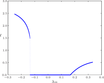
Our MF analysis thus confirms the qualitative results from the preceding section that already in the simplest model there is both a ferromagnetic and an anti-ferromagnetic transition. This is qualitatively consistent with the phase diagram Fig. 3 restricted to the horizontal axis.
IV.2 Two Couplings
Even for the simple model of the previous subsection no explicit expression is known for as the group integrals cannot be evaluated in closed form (a fact well known from strong-coupling expansions, see e.g. Montvay and Münster (1994)). Things naturally become worse if additional couplings are turned on. Already for two couplings i.e. the action (39), the only way to proceed is by means of numerical methods.
In order to obtain the MF version of the phase diagram Fig. 3 we have employed the following algorithm:
-
1.
At the extremal points of (63) all sources occurring in (58) can be eliminated in favour of the expectation values as in (64). Since the character target space is compact it can be easily discretised defining measures and at each point. Using these measures expectation values can now be computed which in general will differ from . Hence, we first look for local minima of
(76) with norm . These minima, however, do not correspond to exact solutions yet but rather serve as the starting points of a recursion.
-
2.
We now solve the equation for and by Newton iteration using the local minima of the previous step as initial input. In this way we end up with multiple solution vectors each extremising (63).
-
3.
The solution vector with minimal contains the desired ground state expectation values.
We conclude this section with some remarks concerning our choice of the sources . Allowing them to be complex yields an 8-dimensional parameter space for the observables of model (39) with two characters, and . For this large parameter space it would actually be simpler to perform a high-precision Monte Carlo simulation than to find a good approximation for the global minima of (63). For this reason, we have chosen real sources as an input to our MF approximation. We expect this to be a very good approximation as long as the peak of the probability distribution for is concentrated near the real axis in Fig. 2.
Comparing with the classical analysis we note that our real-source assumption is justified for all couplings which are located away from the boundary between the phases F and AC. The F-AC transition should be second order according to the analysis of Section III while the MF approximation with real sources predicts a first order transition (see Fig. 4). The contradiction will be finally resolved by Monte Carlo simulations showing that near the F-AC transition the peaks of the probability distribution for are off the real axis. Apart from this fairly small region in parameter space we find a remarkable agreement between the MF results and the Monte Carlo results of the next section. This provides the ultimate justification for our simplifying choice of real sources in the MF approximation.
V Monte Carlo Simulation
The previous two sections have provided us with a good deal of information on the phase structure of the effective model in the most interesting regions of parameter space. Based on this we have performed a large number of Monte Carlo simulations to quantitatively check the MF predictions and obtain a precise picture of the critical behaviour. As before, to avoid excessive complexity, we have concentrated on the action (39) with two couplings and .
At the beginning of Section IV we have already noted that both the action and the reduced Haar measure depend only on the conjugacy class of the (untraced) Polyakov loop. Hence, one can choose the basic field variables either as the traces in the fundamental representations (, ) and powers thereof or as a suitable parametrisation in terms of the eigenvalues as introduced in (40). It turns out that for a numerical treatment the latter proves to be more appropriate and so we use (40) to represent the conjugacy class according to
| (77) |
Here, the following restrictions should be imposed such that the angular coordinates cover each class only once,
| (78) |
These restrictions are somewhat awkward to implement in a simulation code. It is much more convenient to let take values in the full square which covers the fundamental domain given by (78) six times. Due to the residual gauge symmetry of the system it is clear that expectation values will be unaffected by this over-counting.
In the coordinates (77) the reduced Haar measure becomes
| (79) |
where the normalization is such that the measure integrates to unity over the square . All characters can be expressed in terms of and . Using (79) the full measure (49) may be straightforwardly expressed in terms of the angular coordinates as
| (80) |
The focus of our numerical studies has been the phase diagram in the plane. There, we have scanned through the region with a resolution of points, which were in total different Monte Carlo simulations. Before we present our results a few words on our numerical techniques are in order.
V.1 Algorithms
For the investigation of phase transitions, in particular their order, histogram methods are widely used and accepted. This approach, however, requires large statistics and thus tends to consume a lot of computer time. In addition, we are interested in a fairly large range of coupling constants. For these reasons, the updating algorithm for the Polyakov loop models has to be fast and versatile. It turns out that the standard Metropolis algorithm favourably matches both requirements if we aim at an accuracy of about . On the other hand, because of the highly nontrivial probability measure involved, a heat bath algorithm does not seem applicable or, in any case, would be too time consuming. In addition, its local nature should not yield any enhancement of statistics near a first order phase transition. We have thus refrained from implementing a heat bath update scheme but rather decided to optimise the Metropolis algorithm as described in the following two paragraphs.
V.1.1 Multicanonical algorithm
When a system undergoes a first order phase transition, the histogram associated with the order parameter will generically display a multi-peak structure. Depending on the total volume of the system the peaks can be very pronounced. In other words, the configuration space is decomposed into distinct sectors between which local algorithms can hardly mediate. One way to overcome the resultant failure in sampling the total configuration space is to make use of the multicanonical algorithm, see e.g. Berg (2000).
The crucial improvement step consists in the replacement of the measure used in (80) according to
| (81) |
The new improved measure on the right-hand side has a weight which depends on the (modulus of the) order parameter. One chooses the particular form
| (82) |
where denotes the probability density of the order parameter. This choice leads to an enhancement of configurations that would otherwise be suppressed and thus allows for a much improved ergodic behaviour of the algorithm.
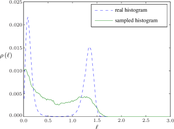
The effect due to the altered measure is illustrated in Fig. 6 where two typical distributions are plotted. In the original distribution one clearly recognises two well-separated peaks. Any local algorithm will fail to sample such a distribution properly once it is trapped at one of its peaks. The distribution actually used ‘closes the gap’ enabling transitions between different peak regions during the simulation. In the end, of course, one has to correct for the change in the measure by reweighting with ,
| (83) |
where we have denoted expectation values taken with respect to the modified measure with a subscript ‘mult’.
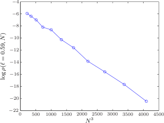
A slight problem with this approach, however, still has to be overcome. One actually needs right at the beginning what one set out to compute originally, namely the distribution . A practicable strategy is e.g. the following. From a small lattice volume, say , where peaks are usually less pronounced, one obtains an approximate distribution function which is then used on a slightly bigger lattice, say of volume . This simple trick can be further refined if on the larger lattice one first computes using and subsequently repeats all measurements employing . In practice, this procedure is iterated several times to make larger and larger lattices available. Going beyond a volume of requires additional knowledge of the scaling behaviour of . Fig. 7 shows that, to a very good approximation, the scaling depends linearly on the volume, ,
| (84) |
In summary, the multicanonical algorithm yields substantial improvements compared to the standard Metropolis algorithm and allows for very accurate simulations. Lattices with volumes up to could thus be studied near the first order phase transition. However, as the implementation is very involved we applied it only to the minimal model (). In principle, the generalisation to incorporating further couplings is straightforward, being merely a matter of having sufficient computing time available.
V.1.2 Cluster algorithm
The multicanonical algorithm is best suited for studying first order transitions. This is no longer true for second order transitions where it is outperformed by cluster algorithms – at least if there is one available. For our purposes, none of the algorithms on the market could be immediately put to use. We therefore decided to modify the well-known Wolff algorithm Wolff (1989), an extension of the Swendsen-Wang Swendsen and Wang (1987) algorithm originally proposed for discrete spin systems.
Before actually describing our modifications let us briefly recall the main idea of Wolff (1989). Suppose the action (and the measure) are invariant under a certain global symmetry which acts on the fields according to
| (85) |
Typically, the symmetry operator will depend on some parameters which we collectively denote by (continuous or discrete) so that . It is important to note that the operator has to be idempotent, , in order to ensure detailed balance. The algorithm then works according to the following list.
-
1.
Fix some parameter and hence some transformation . Randomly choose a lattice point and apply the symmetry transformation
(86) which may be viewed as flipping the field variable . The point is checked and added to the cluster.
-
2.
Repeat the following for all unchecked neighbours of :
Let denote the contribution to the action from the link and compute
(87) which may be rewritten as
(88) since is already invariant under . The decision to add to the cluster is subject to an accept/reject step so that the probability to flip becomes
(89) If is flipped, check the point .
-
3.
Go back to Step (2) for all sites added to the cluster in the previous step.
Note that (88) measures whether it is advantageous to flip once has been flipped. From the very construction of the algorithm it should be already clear that the clusters will increase with the correlation length of the system. In this way one suppresses the phenomenon of critical slowing down observed with local algorithms. This makes the cluster algorithm particularly suited for the study of second order phase transitions.
The first step in adapting the cluster algorithm to our needs is to find suitable symmetries of the action (21). Being a Polyakov loop model the symmetry in question is the discrete symmetry, . In addition, the action has to be real which implies constraints on the way complex conjugation acts. From these symmetries one can construct three operators , , acting on the Polyakov loop according to
| (90) |
As required the square to unity. Furthermore, it is easy to see that both the operators appearing in (26) and the domain of the Polyakov loop are left invariant by the action of . The latter is illustrated in Fig. 8 for a particular value of .
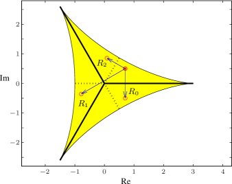
For the actual algorithm the transformations (90) are not immediately applicable since the simulation is based on the angular variables introduced in (77). However, it is just a matter of a little algebra to show that the act on the angles via
| (91) |
Whereas in the original cluster algorithm flipping along randomly chosen lattice sites is sufficient to guarantee ergodicity this is no longer true in the present case. Hence, we have to augment the update scheme by standard Metropolis sweeps to make the algorithm ergodic. For one Monte Carlo step our cluster algorithm finally can be summarised as follows:
-
1.
Choose a random number between and .
-
2.
Do standard Metropolis sweeps at randomly drawn lattice points.
-
3.
For a suitable fixed number repeat the steps for building a cluster as described above.
-
4.
Do additional Metropolis sweeps, again at randomly chosen lattice sites.
From several test runs we have found that the number should be chosen such that total number of flipped sites after performing step (3) is approximately half the number of all lattice sites. Thus, if denotes the typical size of a cluster, the following equation should hold (at least approximately),
| (92) |
One of the most interesting questions of course is the gain in performance compared to e.g. the standard Metropolis algorithm. We have found that the autocorrelation time for the order parameter is independent of both the lattice extent (at least in the range ) and the coupling constant (if close to the second order phase transition) implying a dynamical critical exponent of . Moreover, for an optimal choice of the autocorrelation time is of order unity. As a result, our cluster algorithm outperforms the Metropolis algorithm even for small lattices. On the largest lattices we have considered the cluster algorithm reduces autocorrelation times by two orders of magnitude as compared to Metropolis updating. This improvement comes at the cost of a slightly increased complexity, specifically a factor of 1.5 in computing time which clearly is negligible. On the other hand, in line with our expectations, no significant improvement has been found near the first order transition.
V.2 Results
We present the results of our Monte Carlo simulations in the same two steps as for the MF approximation. Hence, we first report on the minimal model (66) and switch on later on. With only different from zero it is reasonably cheap to perform highly accurate measurements so that a precise quantitative comparison with the 3-state Potts model is possible.
For the model (39) with two couplings we determine the phase diagram in the – plane and compare with our expectations as laid out in the previous two sections. We conclude with a careful study of the nature of the phase transitions, in particular their continuity properties.
V.2.1 Minimal model (one coupling)
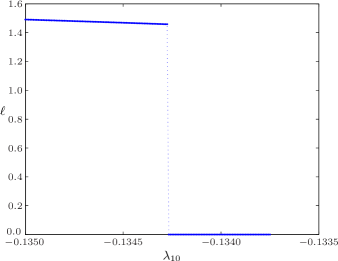
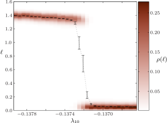
To determine the ferromagnetic phase transition for we have used standard techniques which need no further explanation. It suffices to note that in order to study the first order (S-F) transition we performed sweeps on a -lattice in the multicanonical ensemble for each value of the coupling constant. This led to highly accurate statistics until we approached the close vicinity of the critical coupling itself. In this regime our statistics is restricted to independent samples due to large correlation times of the order of sweeps. As Fig. 10 shows this is sufficient to demonstrate that the transition is first order.
In Fig. 9 we compare our Monte Carlo result for with its MF approximation. The figure basically zooms into that part of Fig. 5 where the first order ferromagnetic transition is located. Again, the first order nature of the transition is corroborated.
In addition to the coupling dependence of the order parameter we have determined both the critical coupling and the discontinuity at . The results are given in Table 1 together with the MF prediction. Again we find a surprisingly good quantitative agreement between simulations and MF approximation. Moreover, if we consider the ratio of the two critical couplings, say , we are able to compare this with results of the 3-state Potts model. The actual figures turn out to be fairly close, namely for the minimally coupled Polyakov model and for the 3-state Potts model Janke and Villanova (1997); Gottlob and Hasenbusch (1994).
| method | (S-F) | (S-AF) | |
|---|---|---|---|
| Monte Carlo | |||
| Mean Field |
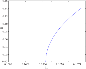
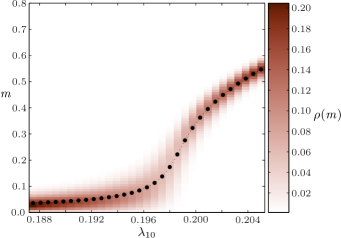
Table 1 also displays the (positive) critical coupling for the second order AF transition. This has been analysed with our modified cluster algorithm by performing a total number of sweeps. With these large statistics at hand it is also possible to determine some of the critical exponents thus probing the universality properties of the model. To do so we have employed standard renormalisation group techniques following Gottlob and Hasenbusch (1993). In particular, we consider the Binder cumulant and susceptibility given by
| (93) | ||||
| (94) |
with as defined in (71) and denoting the spatial extent of the lattice as before.
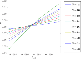
The Binder cumulant is constructed such that it becomes independent of close to the critical point. Hence, the latter is rather precisely determined as the point where the graphs of (plotted for different ) intersect. This behaviour is nicely exhibited in Fig.13.
From the standard relations at criticality,
| (95) | |||
| (96) |
we have finally computed the critical exponents and which are listed in Table 2.
| exponent | 3-state Potts Gottlob and Hasenbusch (1994) | minimal Polyakov |
|---|---|---|
The uncertainty in quoted in Table 1 is mainly due to the fact that the different cumulants do not precisely meet in a single intersection point (cf. again Fig. 13). The error in the critical exponents is estimated from a least square fit to the logarithm of (95) and (96). To cross-check our results we have measured the expectation value of and its probability distribution in analogy with the ferromagnetic transition already discussed. As in the former case, the expectation value of the order parameter alone does not suffice to decide on the order of the transition. However, the probability distribution shown in Fig. 12 is quite different from the one in Fig. 10. No discontinuous behaviour is observed now which provides further (numerical) evidence for a second order phase transition. Equally important, the critical coupling obtained is compatible with the results presented in Table 1. For the sake of completeness Fig. 11 shows the MF prediction for the transition S-AF.
Comparing with earlier results on the 3-state Potts model Wang et al. (1990) we draw the important conclusion that the minimal Polyakov loop model is in the same universality class.
V.2.2 The phase diagram for two couplings
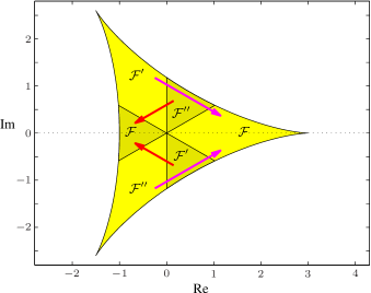
Having discussed the minimal model at length let us continue by switching on the second coupling in order to analyse the phase diagram in the coupling constant plane. This requires a suitably chosen ‘indicator’ to distinguish the (at least) four phases (S, F, AC and AF) we expect in accordance with our MF analysis of Section IV. While and clearly are order parameters for the minimal model they are numerically less suited for the model with two couplings. It turns out advantageous to construct a new observable denoted which may be obtained from by the following procedure. We first divide the domain of into six distinct parts as shown in Fig. 14. The light-shaded region represents the preferred locus of the Polyakov loop in the ferromagnetic phase F, whereas the dark-shaded region corresponds to the anti-centre ferromagnetic phase AC. To eliminate the (numerically superfluous) symmetry the first step in our projection is to identify the regions as indicated by the arrows in Fig. 14. In this way we end up with a fundamental domain for the symmetry centred along the real axis. Every is mapped into by a centre transformation. To finally obtain a real observable we project the transformed onto the real axis. This projection results in the variable the sign of which clearly distinguishes between the two ferromagnetic phases. indicates the AC phase, the ferromagnetic phase F, while in the symmetric phase S. Mathematically, the projection of to is given by
| (97) |
To detect the AF phase we simultaneously measure so that we can finally discriminate between all possible phases.
Our main results for the phase diagram are shown in Fig. 15 obtained by the modified MF approximation explained earlier and Fig. 16 which displays the Monte Carlo data and hence constitutes the most faithful representation of the phase structure.
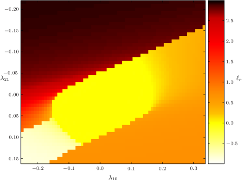
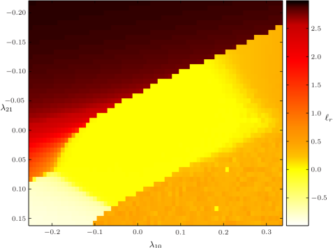
The Monte Carlo simulations were carried out on a -lattice. The number of sweeps was chosen such as to reduce the jackknife error in the estimate of below . The independence of our samples was ensured by demanding that the autocorrelation time associated with the observable was less then one percent of the total number of sweeps. As a result our simulations included at least sweeps far away from the critical regions and more than sweeps in their vicinity.
It is reassuring to note that the qualitative phase diagram Fig. 3 predicted from energy-entropy arguments is quantitatively confirmed by both Figs. 15 and 16. Comparing the latter in some detail it is once more remarkable how good the MF approximation works. Within large regions of parameter space it agrees with the ‘real’ data within 10% or less. Interestingly, the observable also seems to be sensitive to the AF phase (see lower right part of Figs. 15 and 16). However, any further discrimination between phases F and AF by means of is impossible. To lift this degeneracy one clearly needs the AF order parameter as an additional input.
It remains to be discussed why is sensitive at all to AF ordering. In what follows we will provide a heuristic answer in the context of the 3-state Potts model. By definition, all spins are (anti)aligned in the (anti)ferromagnetic ground state. In the symmetric Ising model with only two spin states each possible ground state is two-fold degenerate, independent of the particular ordering (F or AF). The counting of degeneracies, however, is totally different for systems with more spin states (hence higher symmetry). In the AF phase the additional freedom of choice between two (or more) states anti-aligned with a given one leads to an enormous degeneracy of the ground state in energy. As a consequence, entropy will be the sole judge deciding what is to be observed in a measurement. For the Polyakov loop model both MF approximation and the Monte Carlo simulations tell us that the most probable ground state corresponds to a preferred direction for the Polyakov loop on one of the two sub-lattices and an equal distribution of the two remaining directions on the other sub-lattice. Although we do not have an analytical justification for this statement the numerical evidence is compelling. Based on the latter, the sensitivity of to AF ordering can be explained by a net expectation value which for the case of the 3-state Potts model is easily computed as
| (98) |
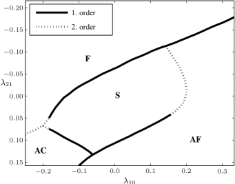
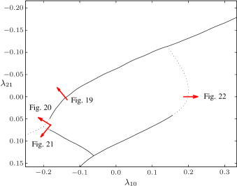
We conclude this discussion with an overview of the resulting phases, their boundaries and the order of the transitions in between presented in Fig. 17. Our reasoning here is based on additional measurements carried out along parametrised curves as depicted in Fig. 18. These simulations were exclusively focused on the order of the phase transition measuring the histograms of the observables and . As before all measurements were carried out on -lattices each trajectory being sampled with twenty points. For every such point Monte Carlo sweeps were performed. To improve the statistics of the histograms we made use of all previously discussed symmetries (, complex conjugation and exchange of even and odd sub-lattice) by binning or together with their centre images , , , and their complex conjugates. This amounts to using each measured value of six times and of even twelve times. In total we have recorded twenty such runs four of which are depicted in Fig. 18.
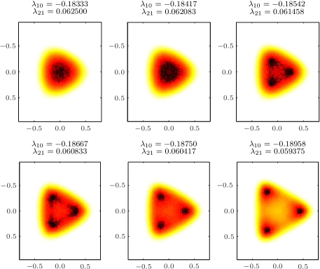
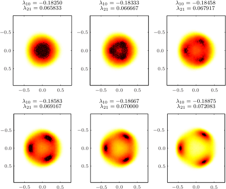
To illuminate the order of the transitions corresponding to the four directed line crossings displayed in Fig. 18 we present six (out of twenty) histograms in Figs. 19 to 22 which display the distribution of the observable respectively in the complex plane.
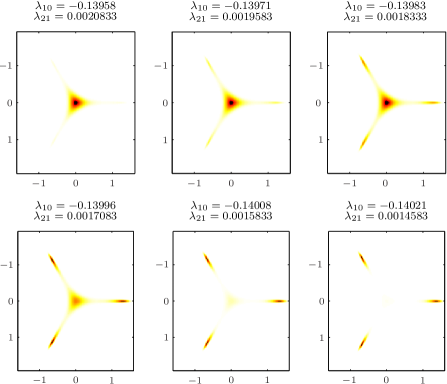
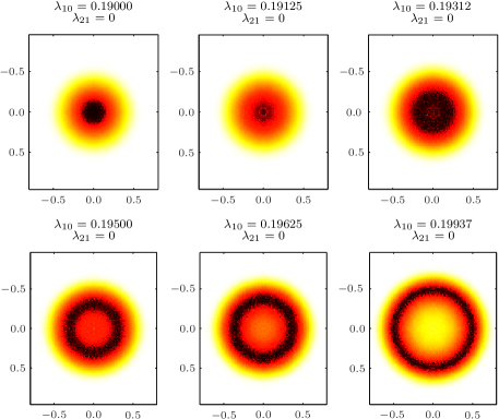
The first figure in this series, Fig. 19, corresponds to the ferromagnetic transition, S-F. The histograms displayed may be viewed as a ‘movie sequence’ starting out in the symmetric phase with the distribution located at the origin. Recalling the relation between probability distribution and the constraint effective potential O’Raifeartaigh et al. (1986), , this situation corresponds to a unique minimum of at . As the couplings change three further maxima – which are copies of each other – arise in addition to the one at the origin. Hence, we observe coexistence of ordered and disordered phases. The new maxima are separated from the original unique maximum at the origin by a finite amount. The associated discontinuity together with coexistence clearly shows that the transition is first order.
In contrast to this the situation depicted in Fig. 20 is quite different. First of all the distribution is much more delocalised as compared to Fig. 19 implying a much flatter effective potential. Moreover, as soon as the maxima of the broken (ordered) phase emerge the maximum at the origin has dissolved. Hence, there is no coexistence of different phases as in the previous case but rather a continuous appearance of new maxima, branching away from the origin towards the corners of the fundamental domain. These features characterise a second order phase transition.
Analogous behaviour can be observed in Fig. 21 with the maxima now moving in roughly the opposite directions indicating a transition to the AC phase. Still different is the S-AF transition of Fig. 22. By the same reasoning as given above this transition is of second order as well. However, the probability function emerging in the broken phase does not display the usual three-fold symmetry we have observed for the previous transitions. Although the figures seemingly look rotationally invariant one actually finds a six-fold degeneracy rather than a continuous one. The symmetry enhancement by a factor of two has a simple explanation. Note that Fig. 22 shows the probability distribution of the AF order parameter which is defined in terms of even and odd sub-lattices. Interchanging the latter accounts for the additional factor of two.
Let us conclude this section with a short remark concerning Figs. 20 and 21. We have seen that our numerical data seem to indicate the possibility of second order transitions from the disordered phase S to F or AC ordering. This is at variance with the folklore claiming the absence of a universality class in , see e.g. Holland et al. (2004a). It is not excluded that the observed second order characteristics near the tricritical point (S-F-AC) derive from artifacts due to our algorithms. At the moment, however, we cannot make a definite statement about this issue. Obviously, the puzzle deserves further investigation in the future.
VI Summary and Outlook
As outlined in the introduction the original motivation for Polyakov loop models lies in their status as effective theories for finite-temperature gluodynamics. However, our investigation of the statistical mechanics involved should have made it clear that they are interesting in their own right. In support of this statement we mention the 3-fold symmetry shared with the 3-state Potts model, the nontrivial complex target space and the enormously rich phase structure resulting thereof.
As we have seen, the latter can be understood qualitatively by simple energy-entropy considerations which predict a symmetric phase S close to the origin in coupling space ‘surrounded’ by broken phases. These can exhibit ferromagnetic (F), anti-ferromagnetic (AF) or anti-centre (AC) ordering. This picture has been confirmed quantitatively both within a mean-field (MF) approximation and by extensive Monte Carlo simulations. Both methods find a first order transition for S-F and a second order one for S-AF. In order to capture the details of the phase diagram a total number of 8000 simulations (corresponding to roughly 3000 hours of CPU time) was required. Naturally, this has added further refinements to our classical and MF analysis like precise values for critical couplings and exponents.
The agreement between MF and Monte Carlo result is much better than naively expected for a statistical model in . The S-F critical couplings agree to within 1%, the discontinuity within 10% and the S-AF critical coupling within 20%. The precise agreement for the S-F transition suggests that the point where the S-F and S-AC critical lines merge is actually a tricritical point where two first order transitions merge into a second order one. It is known that the upper critical dimension for a tricritical point is three Lipowsky and Seifert (1985); Lawrie and S.Sarbach (1984) so that in the MF approximation actually is exact apart from logarithmic corrections Landau and Swendsen (1986). This observation is corroborated by the fact that the Polyakov loop model with two couplings is somewhat similar to the spin-one Blume-Capel Blume (1966); Capel (1966) model which apart from an Ising term has an addition , , with 3 spin states. The model is known to have a tricritical point and is closely related to the 3-state Potts model Landau and Swendsen (1991). The second order phase transition line is characterised by 3 Ising critical exponents. Obviously, one should test the analogous exponents for our AC-F transition at the very left of our phase diagrams.
One may also address the spatial localisation of the phases. On the 3 lattice the coexisting phases should be separated by interfaces the tension of which can be measured (see e.g. Holland and Wiese (2000) and references therein).
In the end one is of course interested in matching the effective couplings to the underlying microscopic theory, i.e. finite-temperature Yang-Mills. The resulting curve in the space of effective couplings should stay in the symmetric and ferromagentic phases. We have already solved the matching-problem for the (simpler) case of using inverse Monte Carlo methods based on Schwinger-Dyson equations. For this is considerably more difficult (at least technically) due to the increased complexity of the Haar measure. The problem is actually similar to one encountered in strong-coupling expansions where group integrals can be performed analytically which is no longer true for . Nevertheless, we have been able to derive the relevant Schwinger-Dyson equations and hope to report on their applications in the near future.
VII Acknowledgements
We thank Guy Buss for his contributions to the strong coupling expansion and Georg Bergner, Wolfhard Janke and Erhard Seiler for valuable hints. TK acknowledges support by the Konrad-Adenauer-Stiftung e.V., CW by the Studienstiftung des deutschen Volkes and TH by the Plymouth Particle Theory Group.
References
- Yaffe and Svetitsky (1982) L. G. Yaffe and B. Svetitsky, Phys. Rev. D26, 963 (1982).
- Svetitsky and Yaffe (1982) B. Svetitsky and L. G. Yaffe, Nucl. Phys. B210, 423 (1982).
- Engels et al. (1990) J. Engels, J. Fingberg, and M. Weber, Nucl. Phys. B332, 737 (1990).
- Engels et al. (1992) J. Engels, J. Fingberg, and D. E. Miller, Nucl. Phys. B387, 501 (1992).
- Holland et al. (2004a) K. Holland, M. Pepe, and U. J. Wiese, Nucl. Phys. B694, 35 (2004a), eprint hep-lat/0312022.
- Celik et al. (1983) T. Celik, J. Engels, and H. Satz, Phys. Lett. B125, 411 (1983).
- Kogut et al. (1983) J. B. Kogut et al., Phys. Rev. Lett. 50, 393 (1983).
- Gottlieb et al. (1985) S. A. Gottlieb et al., Phys. Rev. Lett. 55, 1958 (1985).
- Brown et al. (1988) F. R. Brown, N. H. Christ, Y. F. Deng, M. S. Gao, and T. J. Woch, Phys. Rev. Lett. 61, 2058 (1988).
- Fukugita et al. (1989) M. Fukugita, M. Okawa, and A. Ukawa, Phys. Rev. Lett. 63, 1768 (1989).
- Alves et al. (1990) N. A. Alves, B. A. Berg, and S. Sanielevici, Phys. Rev. Lett. 64, 3107 (1990).
- Pisarski (2000) R. D. Pisarski, Phys. Rev. D62, 111501 (2000), eprint hep-ph/0006205.
- Pisarski (2002) R. D. Pisarski, Nucl. Phys. A702, 151 (2002), eprint hep-ph/0112037.
- Dumitru et al. (2004) A. Dumitru, Y. Hatta, J. Lenaghan, K. Orginos, and R. D. Pisarski, Phys. Rev. D70, 034511 (2004), eprint hep-th/0311223.
- Holland and Wiese (2000) K. Holland and U.-J. Wiese (2000), in At the Frontier of Particle Physics — Handbook of QCD, M. Shifman, ed., World Scientific, Singapore, 2001, eprint hep-ph/0011193.
- Holland et al. (2004b) K. Holland, M. Pepe, and U. J. Wiese, Nucl. Phys. Proc. Suppl. 129, 712 (2004b), eprint hep-lat/0309062.
- Holland et al. (2003) K. Holland, P. Minkowski, M. Pepe, and U. J. Wiese, Nucl. Phys. B668, 207 (2003), eprint hep-lat/0302023.
- Borgs and Seiler (1983) C. Borgs and E. Seiler, Commun. Math. Phys. 91, 329 (1983).
- Ford et al. (1999) C. Ford, T. Tok, and A. Wipf, Phys. Lett. B456, 155 (1999), eprint hep-th/9811248.
- Meisinger et al. (2002) P. N. Meisinger, T. R. Miller, and M. C. Ogilvie, Phys. Rev. D65, 034009 (2002), eprint hep-ph/0108009.
- Dittmann et al. (2004) L. Dittmann, T. Heinzl, and A. Wipf, JHEP 06, 005 (2004), eprint hep-lat/0306032.
- Heinzl et al. (2005) T. Heinzl, T. Kaestner, and A. Wipf, Phys. Rev. D72, 065005 (2005), eprint hep-lat/0502013.
- Polonyi and Szlachanyi (1982) J. Polonyi and K. Szlachanyi, Phys. Lett. B110, 395 (1982).
- Ogilvie (1984) M. Ogilvie, Phys. Rev. Lett. 52, 1369 (1984).
- Billo et al. (1996) M. Billo, M. Caselle, A. D’Adda, and S. Panzeri, Nucl. Phys. B472, 163 (1996), eprint hep-lat/9601020.
- Svetitsky (1986) B. Svetitsky, Phys. Rept. 132, 1 (1986).
- Buss (2004) G. Buss (2004), diploma thesis, Jena (in German).
- Creutz (1983) M. Creutz, Quarks, Gluons and Lattices, Cambridge Monographs on Mathematical Physics (Cambridge University Press, 1983).
- Montvay and Münster (1994) I. Montvay and G. Münster, Quantum Fields on a Lattice, Cambridge Monographs on Mathematical Physics (Cambridge University Press, 1994).
- Jensen and Mouritsen (1979) S. J. K. Jensen and O. G. Mouritsen, Phys. Rev. Lett. 43, 1763 (1979).
- Kogut and Sinclair (1982) J. B. Kogut and D. Sinclair, Solid State Commun. 41, 187 (1982).
- Wu (1982) F. Y. Wu, Rev. Mod. Phys. 54, 235 (1982).
- Potts (1952) R. Potts, Proc. Camb. Phil. Soc. 48, 106 (1952).
- Janke and Villanova (1997) W. Janke and R. Villanova, Nucl. Phys. B489, 679 (1997), eprint hep-lat/9612008.
- Gottlob and Hasenbusch (1994) A. P. Gottlob and M. Hasenbusch, Physica A210, 217 (1994).
- Wang et al. (1990) J.-S. Wang, R. H. Swendsen, and R. Kotecký, Phys. Rev. B42, 2465 (1990).
- Berg (2000) B. A. Berg, Fields Inst. Commun. 26, 1 (2000), eprint cond-mat/9909236.
- Wolff (1989) U. Wolff, Phys. Rev. Lett. 62, 361 (1989).
- Swendsen and Wang (1987) R. H. Swendsen and J.-S. Wang, Phys. Rev. Lett. 58, 86 (1987).
- Gottlob and Hasenbusch (1993) A. P. Gottlob and M. Hasenbusch (1993), eprint cond-mat/9305020.
- O’Raifeartaigh et al. (1986) L. O’Raifeartaigh, A. Wipf, and H. Yoneyama, Nucl. Phys. B271, 653 (1986).
- Lawrie and S.Sarbach (1984) I. Lawrie and S.Sarbach, pp. 2–155 (1984), in: C. Domb and J.L. Lebowitz, editors, Phase Transitions and Critical Phenomena, Vol. 9, chapter 1, pages 2-155. Academic Press, New York.
- Lipowsky and Seifert (1985) R. Lipowsky and U. Seifert, Phys. Rev. B 31, 4701 (1985).
- Landau and Swendsen (1986) D. Landau and R. Swendsen, Phys. Rev. B 33, 7700 (1986).
- Blume (1966) M. Blume, Phys. Rev. 141, 517 (1966).
- Capel (1966) H. Capel, Physica 32, 966 (1966).
- Landau and Swendsen (1991) D. Landau and R. Swendsen, Phys. Rev. Lett. 46, 1437 (1991).