Excited hadrons on the lattice: Baryons

Abstract

We present results for masses of excited baryons from a quenched calculation with Chirally Improved quarks at pion masses down to 350 MeV. Our analysis of the correlators is based on the variational method. In order to provide a large basis set for spanning the physical states, we use interpolators with different Dirac structures and Jacobi smeared quark sources of different width. Our spectroscopy results for a wide range of ground state and excited baryons are discussed.

I Introduction

The reproduction of the hadron mass spectrum from first principles is an important challenge for lattice QCD. Ground state spectroscopy on the lattice is by now a well understood problem and impressive agreement with experiments has been achieved. However, the lattice study of excited states excitedspectro –exmeson is not as advanced. The reason for this is twofold: Firstly, the masses of excited states have to be extracted from subleading exponentials in the spectral decomposition of two-point functions. Secondly, the construction of hadron interpolators which have a good overlap with the wave functions of excited states is much more challenging than for the ground state.

Concerning the first issue, the extraction of the signal from the subleading exponential, several approaches such as constrained fitting or the maximum entropy method can be found in the literature constrainedfits ; maximumentropy . Here we apply the variational method Mi85 ; LuWo90 , where not only a single correlator is analyzed, but a matrix of correlators is used. This matrix is built from several different interpolators, all with the quantum numbers of the desired state. The variational method also incorporates in a natural way a solution to the second issue, the wave function of the excited states: One uses a set of basis interpolators which is large enough to span ground and excited states and the variational method finds the optimal combinations of them. In principle, no prior knowledge of or assumption about the composition of the physical hadron state has to be used.

However, the variational method can succeed only if the basis set of hadron interpolators is rich enough to span ground and excited states. On the other hand, the basis should also be constructed such that it can be implemented numerically in an efficient way without the need for many different quark sources. In this article we use a twofold strategy for building our basis interpolators: We use interpolators with different Dirac structures and furthermore compose them using different types of smearing for the individual quarks. In particular, we apply different amounts of Jacobi smearing jacobi and in this way create “narrow” and “wide” sources. A combination of these allows for spatial wave functions with nodes, which are essential for a good overlap with excited states.

Following a first test of the outlined strategy firsttest and an analysis of mesons with our method exmeson , in this paper we present in detail the results obtained for baryons. In the next section we collect the basic equations for the implementation of the variational method, detail the construction of our sources and give an overview of the parameters of our numerical simulation. Subsequently we discuss effective mass plots, the eigenmodes of the correlation matrix, as well as the baryon masses and their chiral extrapolations. The paper closes with a summary and an outlook.

II Outline of the calculation

II.1 The variational method

As already stated, we use the variational method Mi85 ; LuWo90 to extract the masses of ground and excited states. Starting from a set of basis operators $O_{i},\,i=1,2\,...\,N$, we compute the correlation matrix

$$C_{ij}(t)\;=\;\langle\,O_{i}(t)\,\overline{O}_{j}(0)\,\rangle\;.$$ (1)

In Hilbert space these correlators have the decomposition

$$C_{ij}(t)\;=\;\sum_{n}\langle\,0\,|\,O_{i}\,|\,n\,\rangle\langle\,n\,|\,O_{j}^{\dagger}\,|\,0\,\rangle\,e^{-t\,M_{n}}\;.$$ (2)

Using the factorization of the amplitudes one can show LuWo90 that the eigenvalues $\lambda^{(k)}(t)$ of the generalized eigenvalue problem

$$C(t)\,\vec{v}^{\,(k)}\;\;=\;\;\lambda^{(k)}(t)\,C(t_{0})\,\vec{v}^{\,(k)}\;,$$ (3)

behave as

$$\lambda^{(k)}(t)\;=\;e^{-(t-t_{0})\,M_{k}}\,[\,1+{\cal O}(e^{-(t-t_{0})\,\Delta M_{k}})\,]\;,$$ (4)

where $M_{k}$ is the mass of the $k$-th state and $\Delta M_{k}$ is the difference to the masses of neighboring states. In Eq. (3) the eigenvalue problem is normalized with respect to a timeslice $t_{0}<t$.

At this point we remark, that the variational method can be generalized to include also ghost contributions as they appear in a quenched or partially quenched calculation. The fact that ghost contributions play a role also for baryons was first stressed in excitedspectro . In the spectral decomposition (2) ghosts appear with a modified time dependence, possibly including also a negative sign. In ghostvar it was shown that the ghost contribution couples to an individual eigenvalue (up to the correction term) in the same way as a “proper” physical state. Thus, ghost contributions are disentangled from the desired states and need not be modeled in the further analysis of the exponential decay of the eigenvalues.

Let us finally stress that also the eigenvectors of the generalized eigenvalue problem (3) contain interesting information. If one plots the entries of the eigenvector as a function of $t$, one finds that they are essentially constant in the same range of $t$-values where plateaus of the effective mass are seen (compare Fig. 2). These plateaus can be used to optimize the interval for fitting the eigenvalues. Furthermore, the eigenvectors encode the information which linear combinations of the basis interpolators couple to which eigenvalue and thus provide one with a “fingerprint” of the corresponding states. Comparing these fingerprints for different values of the quark mass is an important cross-check for the correct identification of the states.

II.2 Dirac structure of the baryon interpolators

For the baryons we analyze, we use the following operators with different Dirac structures:

• Nucleon:

  $$N^{(i)} = \epsilon_{abc}\Gamma^{(i)}_{1}u_{a}(u_{b}^{T}\Gamma^{(i)}_{2}d_{c}-d_{b}^{T}\Gamma^{(i)}_{2}u_{c})\;.$$ (5)

• $\Sigma$:

  $$\Sigma^{(i)} = \epsilon_{abc}\Gamma^{(i)}_{1}u_{a}(u_{b}^{T}\Gamma^{(i)}_{2}s_{c}-s_{b}^{T}\Gamma^{(i)}_{2}u_{c})\;.$$ (6)

• $\Xi$:

  $$\Xi^{(i)} = \epsilon_{abc}\Gamma^{(i)}_{1}s_{a}(s_{b}^{T}\Gamma^{(i)}_{2}u_{c}-u_{b}^{T}\Gamma^{(i)}_{2}s_{c})\;.$$ (7)

• $\Lambda$-octet:

  $$\Lambda_{8}^{(i)} = \epsilon_{abc}\{\Gamma^{(i)}_{1}s_{a}(u_{b}^{T}\Gamma^{(i)}_{2}d_{c}-d_{b}^{T}\Gamma^{(i)}_{2}u_{c})$$

  $$\,\,+\;\Gamma^{(i)}_{1}u_{a}(s_{b}^{T}\Gamma^{(i)}_{2}d_{c})-\Gamma^{(i)}_{1}d_{a}(s_{b}^{T}\Gamma^{(i)}_{2}u_{c})\;.$$

• $\Lambda$-singlet:

  $$\Lambda_{1} = \epsilon_{abc}\Gamma^{(1)}_{1}u_{a}(d_{b}^{T}\Gamma^{(1)}_{2}s_{c}-s_{b}^{T}\Gamma^{(1)}_{2}d_{c})$$

  $$\,\,+\;\mbox{cyclic permutations of}\;u,d,s\;.$$

• $\Delta$:

  $$\Delta_{\mu} = \epsilon_{abc}u_{a}(u_{b}^{T}C\gamma_{\mu}u_{c})\;.$$ (10)

• $\Omega$:

  $$\Omega_{\mu} = \epsilon_{abc}s_{a}(s_{b}^{T}C\gamma_{\mu}s_{c})\;.$$ (11)

Here we used vector/matrix notation for the Dirac indices. The different possible choices for $\Gamma^{(i)}_{1}$ and $\Gamma^{(i)}_{2}$ are listed in Table 1.

	$\Gamma^{(i)}_{1}$	$\Gamma^{(i)}_{2}$
$i=1$	$\mathds{1}$	$C\gamma_{5}$
$i=2$	$\gamma_{5}$	$C$
$i=3$	$i\mathds{1}$	$C\gamma_{4}\gamma_{5}$

Table 1: Dirac structures used for nucleon, $\Sigma,\,\Xi$ and $\Lambda$-octet, according to Eqs. (5)–(• ‣ II.2).

Our interpolator for the $\Delta$ ($\Omega$) still has overlap with both spin-$\frac{1}{2}$ and spin-$\frac{3}{2}$. Thus, we need a projection to definite angular momentum. We use the continuum formulation of a spin-$\frac{3}{2}$ projection for a Rarita-Schwinger field:

$$P^{3/2}_{\mu\nu}(\vec{p}) = \delta_{\mu\nu}-\frac{1}{3}\gamma_{\mu}\gamma_{\nu}-\frac{1}{3p^{2}}(\gamma\cdot p\,\gamma_{\mu}p_{\nu}+p_{\mu}\gamma_{\nu}\gamma\cdot p),$$

where $p_{\mu}$ is the 4-momentum, in our case given by $(\vec{0},m)$. For each component of the projected $\Delta$ ($\Omega$) we compute the correlator and average these 2-point functions over $\mu,\nu=1,2,3$.

Finally, our baryon correlators are projected to definite parity using the projection operator $P^{\pm}=\frac{1}{2}(\mathds{1}\pm\gamma_{4})$. We obtain two matrices of correlators:

$$C^{+}_{ij}(t) = Z_{ij}^{+}e^{-tE^{+}}+Z_{ij}^{-}e^{-(T-t)E^{-}},$$ (12)

where we have projected with $P^{+}$ and

$$C^{-}_{ij}(t) = -Z_{ij}^{-}e^{-tE^{-}}-Z_{ij}^{+}e^{-(T-t)E^{+}},$$ (13)

when using $P^{-}$. These two matrices are combined to

$$C(t) = \frac{1}{2}\left(C^{+}(t)-C^{-}(T-t)\right)\;,$$ (14)

to improve statistics. This gives rise to the final correlator $C(t)$ which we then use in the variational method. The positive parity states are obtained from the correlator at small $t$ running forward in time, while the negative parity states are found at large time arguments, propagating backward in time with $T-t$. As expected, the correlation matrices $C(t)$ are real and symmetric within error bars and we therefore symmetrize the matrices by replacing $C_{ij}(t)$ with $C_{ij}(t)=[C_{ij}(t)+C_{ji}(t)]/2$ before diagonalization.

II.3 Quark sources

In addition to the different Dirac structures, we construct the interpolators listed in the last section from quarks with sources created by different amount of smearing. In particular, we use Jacobi smearing jacobi with two different sets of parameters (number of smearing steps, amplitude of hopping term) to create narrow and wide sources. The shapes of these sources are approximately gaussian with $\sigma\sim 0.27$ fm for the narrow source and $\sigma\sim 0.41$ fm for the wide source. Details of the source preparation and plots of the source shapes can be found in firsttest ; exmeson .

Each quark in our baryon interpolators can either be narrow ($n$) or wide ($w$), giving rise to the following eight combinations for the sources:

$$n(nn)\,,\,n(nw)\,,\,n(wn)\,,\,w(nn)\,,$$

$$n(ww)\,,\,w(nw)\,,\,w(wn)\,,\,w(ww)\;.$$ (15)

In this notation the order of the quark fields is understood as in Eqs. (5) – (11) and the parentheses indicate which quarks are combined in the diquark combination. Since the smearing used here is a purely scalar operation, the assignment of quantum numbers, as given in the last subsection, remains unchanged.

Taking into account the different Dirac structures discussed in the last section, we can work with 24 different interpolators for nucleon, $\Sigma$, $\Xi$ and $\Lambda$-octet. For the $\Lambda$-singlet and the $\Delta$ we have only one Dirac structure and consequently a total of 8 different interpolators. We remark that in the final analysis not all interpolators are used. We prune the maximal correlation matrix and remove some of the correlators that couple only weakly to the physical states or add no new information, thus enhancing the numerical noise. The criterion for the selection of the interpolators is the optimization of the quality of the plateaus in the effective mass

$$aM_{eff}^{(k)}\,\Big{(}t+\frac{1}{2}\Big{)}\;=\;\ln\left(\frac{\lambda^{(k)}(t)}{\lambda^{(k)}(t+1)}\right)\;.$$ (16)

II.4 Parameters of the simulation

We work with quenched gauge configurations generated with the Lüscher-Weisz action luweact . We use two sets of lattices, $20^{3}\times 32$ and $16^{3}\times 32$, at couplings $\beta=8.15$ and $\beta=7.90$ corresponding to lattice spacings of $a=0.119$ fm and $a=0.148$ fm, determined from the Sommer parameter in scale . Thus for both lattices we have a spatial extent of $L\sim 2.4$ fm. The two different values of the lattice constant $a$ allow us to assess the cutoff dependence. The parameters of the gauge configurations are collected in Table 2.

Our quark propagators are computed using the Chirally Improved (CI) Dirac operator cioperator . The CI operator is a systematic approximation of a solution of the Ginsparg-Wilson equation giwi with good chiral properties citests . We work with several quark masses in the range $am=0.02,\,...\,0.2$, leading to pion masses down to 350 MeV. For setting the strange quark mass we use the K-meson with the light quark mass extrapolated to the chiral limit.

Our quark sources are placed at $t=0$ and the generalized eigenvalue problem (3) is normalized at $t_{0}=1a$. The final results for the baryon masses were obtained from a fully correlated fit to the eigenvalues. The errors we show are statistical errors determined with single elimination jackknife.

size	$\beta$	confs.	$a$[fm]	$a^{\!-1}$[MeV]
$20^{3}\!\times\!32$	8.15	100	0.119	1680
$16^{3}\!\times\!32$	7.90	100	0.148	1350

Table 2: Parameters of our simulation. We list the lattice size, the inverse coupling $\beta$ the number of configurations, the lattice spacing $a$ and the cutoff $a^{-1}$.

III Results

III.1 Effective masses, eigenvectors and fit ranges

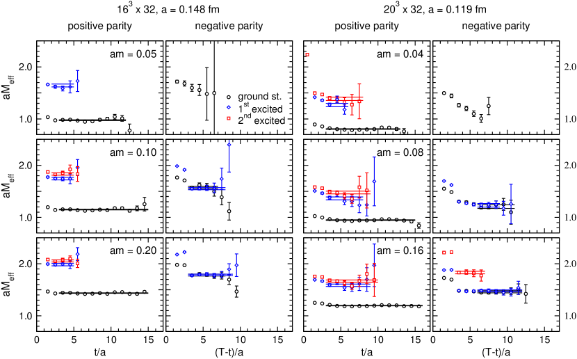
Figure 1: Effective mass plots for nucleon ground and excited states. We compare the results from our coarse ($16^{3}\times 32$, $a=0.148$ fm, $am_{q}=0.05,0.1,0.2$ top to bottom), and fine ($20^{3}\times 32$, $a=0.119$ fm, $am_{q}=0.04,0.08,0.16$) lattices. The solid lines are the results from correlated fits of the eigenvalues. They represent the fit result plus and minus the corresponding error.

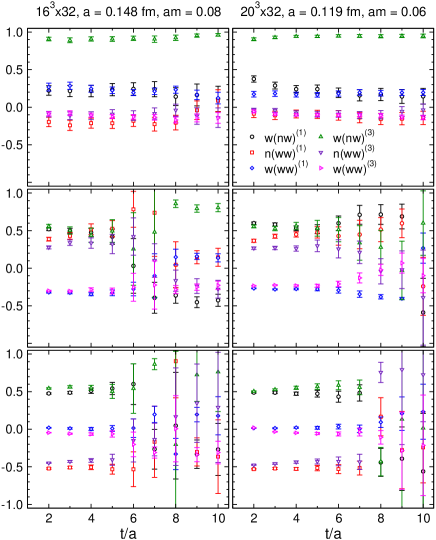
Figure 2: Eigenvectors for nucleon ground and excited positive parity states. From top to bottom we show the eigenvector components of ground, first and second excited state.

Let us begin our presentation with a discussion of effective masses (16) for the nucleon system. For positive parity the combination of the 6 operators $n(ww)^{(1)}$, $w(wn)^{(1)}$, $w(ww)^{(1)}$, $n(ww)^{(3)}$, $w(wn)^{(3)}$, $w(ww)^{(3)}$, (the upper index denotes the choice of Dirac structures according to Table 1) gives the strongest signal. For negative parity we used the $4\times 4$ correlation matrix built from $n(nn)^{(1)}$, $w(nn)^{(1)}$, $n(nn)^{(2)}$, $w(nn)^{(2)}$.

In Fig. 1 we compare the effective mass plots for positive and negative parity nucleons from our two lattices at different values of the bare quark mass; $am=0.05,0.1,0.2$ for $16^{3}\times 32$ and $am=0.04,0.08,0.16$ for $20^{3}\times 32$. These numbers were chosen such that they give rise to approximately equal pion masses for the two lattice spacings used. The plots also contain the nucleon masses in lattice units as obtained from a correlated fit of the propagator (horizontal bars giving the central value plus and minus the statistical error). The figure shows clear long plateaus for the ground state masses, while the signals for excited states have larger error bars and shorter plateaus. Furthermore the quality of the data decreases as the quarks become lighter – a feature well known in lattice spectroscopy.

Another important piece of information comes from the eigenvectors. In Fig. 2 we show the 6 entries of the lowest three eigenvectors corresponding to ground, first and second excited state (top to bottom) in the positive parity nucleon channel. Again we compare the results for our two lattice sizes using quark mass values which give rise to essentially the same pion mass. For each value of $t$ the respective eigenvectors are normalized to unit length.

It is interesting to note that the eigenvectors are only weakly dependent on $t$ (actually this can be shown from the generalized eigenvalue problem). The entries form plateaus which are very long for the ground states but also for the excited states often contain 4 to 8 values of $t$. Typically these plateaus extend at least over the same number of $t$-values as the effective mass plateaus – often they are even longer by one or two points.

As in the case of effective masses, the formation of the eigenvector plateaus indicates that the channel is dominated by a single state. Thus, the eigenvector plateaus provide an important tool for the reliable identification of the $t$-intervals where the eigenvalues can be used for a fit. Indeed, sometimes it is the eigenvectors which prevent one from fitting “quasiplateaus” in the effective mass. Due to relatively large statistical errors in the effective masses, the data sometimes resemble a plateau and it is only the absence of a plateau in the corresponding eigenvectors which allows us to conclude that a quasiplateau is not conclusive. We implemented this strategy and now fit the eigenvalues only where we see also eigenvector plateaus.

We finally remark that the values for the eigenvectors are almost exactly the same for the two values of the cutoff we consider (the left hand side plots are for $a=0.148$ fm, the right hand side is for $a=0.119$). Although the entries of the eigenvectors cannot be expected to scale (they are linear combinations of matrix elements of our interpolators with the physical states), it is reassuring for the application of the method that no large discrepancies are observed.

III.2 Nucleon

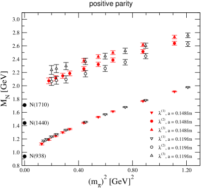
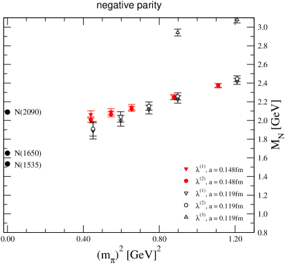
Figure 3: Ground and excited state nucleon masses versus $M_{\pi}^{2}$ for our two lattices. Filled symbols are used for $16^{3}\times 32,\,a=0.148$ fm, open symbols for $20^{3}\times 32,\,a=0.119$ fm. The left hand side plot shows the positive parity states, the right hand side is for negative parity. The experimental data are included as filled circles.

As already discussed in the last section, the positive parity nucleon masses were extracted from the $6\times 6$ correlation matrix of $n(ww)^{(1)}$, $w(wn)^{(1)}$, $w(ww)^{(1)}$, $n(ww)^{(3)}$, $w(wn)^{(3)}$, $w(ww)^{(3)}$, while for negative parity the $4\times 4$ correlation matrix built from $n(nn)^{(1)}$, $w(nn)^{(1)}$, $n(nn)^{(2)}$, $w(nn)^{(2)}$ was used. Of course these combinations were used for all quark masses. For the positive parity ground state we could determine the mass for all our quark masses. For the excited nucleon states of positive parity the combined assessment of effective masses and eigenvector plateaus did not allow for a trustworthy extraction of the corresponding nucleon masses for the two smallest quark masses.

We identify two excited states of positive parity which have not very different masses for the whole quark mass region where we see a signal. This is consistent with our previous observation on a smaller lattice firsttest . These are two physically distinct states since they are observed in different eigenvalues of the correlation matrix and the corresponding eigenvectors are orthogonal. Some additional efforts are required to properly identify the nature of our quenched excited states. We follow the strategy of Ref. firsttest , i.e., we trace the states from the heavy quark region towards the physical limit.

In the heavy quark region, where we obtain the best signals, the quenching and chiral symmetry effects are less important and the naive quark picture is adequate. Then we know a-priori, that there must be two approximately degenerate excited states of positive parity. The first one is a member of the 56-plet of SU(6) and the second one belongs to the 70-plet. In the excited 56-plet state, as well as in the ground state 56-plet (the nucleon), all possible quark pairs have positive parity. Then it follows that the signal from the nucleon, as well as from the excited 56-plet state, can be seen with those interpolators that contain two-quark subsystems of positive parity (these are the ones with $i=1,3$ from the Table I). On the other hand, the positive parity 70-plet state contains both positive and negative parity two-quark subsystems, and can be seen with the $i=2$ interpolator, where the “diquark” has negative parity. This picture is confirmed in the heavy quark limit of our results. If we construct our correlation matrix with the $i=1$ and/or $i=3$ interpolators, we find both the ground state (the nucleon) and two excited states of positive parity, while only one state is observed with the $i=2$ interpolator. This state corresponds to the positive parity excited state.

Using the “fingerprint” from the eigenvectors, we are able to trace these states from the heavy quark region, where their physical nature can be safely identified, to the light quark region (down to $m_{\pi}=450$ MeV), where they still remain approximately degenerate. Clearly these signals, extrapolated to the physical region, remain essentially higher than the experimental states N(1440) and N(1710) (cf. Fig. 3). Phenomenologically the latter states are ascribed to the 56-plet and 70-plet, respectively.

The discrepancy between our results and the experimental numbers is probably partly due to quenching, where a significant part of chiral physics is absent. Also finite volume effects cannot be excluded (our physical volume is 2.4 fm and large finite volume effects can be anticipated for excited states excitedspectro2 ).

Note that the perturbative gluon exchange between valence quarks, characteristic of the naive constituent quark model, is adequately represented in the quenched calculation. The discrepancy of our results with the experimental ones hints that it is the chiral physics, partly missing in quenched QCD, that could shift both positive parity excited states (and especially the Roper state) down GR .

Our results for the nucleons are presented in Fig. 3. The left plot is for positive parity, the right for negative parity. Filled symbols are used for the $16^{3}\times 32,\,a=0.148$ fm lattice, open symbols for $20^{3}\times 32,\,a=0.119$ fm. The filled circles represent the experimental masses.

The results for the positive parity ground state (left plot, downward pointing triangles) agree well with the experimental value (for the chiral extrapolation of our data see Subsection F). Furthermore, the data show almost no cutoff effects. For the first excited state (circles) the results for the two values of the cutoff differ by about one sigma, while for the second excited state (upward pointing triangles) the two data sets agree. However, both excited states extrapolate to values about 20-30% larger than the experimental numbers.

For negative parity we mainly fit ground and first excited states. Only for the two largest quark masses on the finer lattice we can extract the second excited mass. We find that the lowest two states are nearly degenerate, but extrapolate to the physical masses within error bars (compare Subsection F). Cutoff effects are clearly seen only for small quark masses. Since the negative parity ground and first excited state are nearly degenerate, we checked that they are indeed different by inspecting the eigenvectors and following their behavior down from the heavy quark region. Entries of the eigenvectors at quark mass $am=0.06$ are shown for our $20^{3}\times 32$ lattice in Fig. 4. In contrast to the positive parity excited states, the negative parity states fit the experimental data well. This is expected since the negative parity states have the mixed flavor-spin symmetry $[21]_{FS}$ and experience only small chiral effects GR .

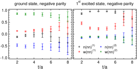
Figure 4: Eigenvectors for nucleon ground and first excited negative parity states. The data are for our $20^{3}\times 32$ lattice at $am=0.06$.

III.3 $\Sigma$ and $\Xi$

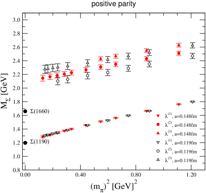
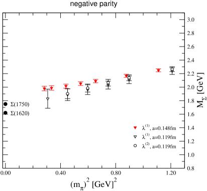
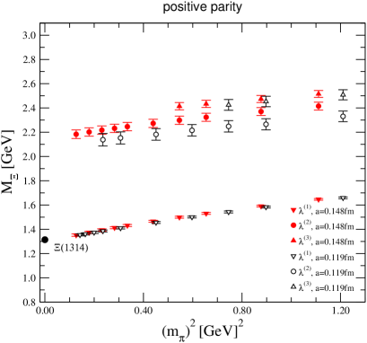
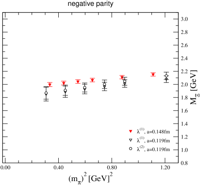
Figure 5: Same as Fig. 3, now for $\Sigma$ and $\Xi$.

Those $\Sigma$ and $\Xi$ resonances which belong to the octet are structurally identical to the nucleon: only one and two, respectively, of the light quarks are replaced by a strange quark. Consequently, their analysis and also the results are only a variation of what has been found for the nucleon system. We use the same combination of interpolators in the $6\times 6$ (for positive parity) and $4\times 4$ (negative parity) correlation matrices as we did for the nucleons.

We present our results for the octet $\Sigma$ and $\Xi$ masses in Fig. 5. As for the nucleon system, the positive parity $\Sigma$ and $\Xi$ ground states are compatible with the experimental numbers and essentially no cutoff effects are visible. Concerning the excited positive parity states, only the first excited states show notable cutoff effects, while the masses of the second excited states from the two lattices are compatible within error bars. For the $\Sigma$, where at least the first excited state is classified, our data extrapolate to a number which is about 20 % larger than the experimental result, similar to the nucleon case.

For negative parity, we find two nearly degenerate states which show clear cutoff effects for the smaller quark masses. For the $\Sigma$ the data are compatible with the known states. For the negative parity $\Xi$ our data extrapolate to two states near 1800 MeV (see also the discussion in Subsection F).

III.4 $\Lambda$

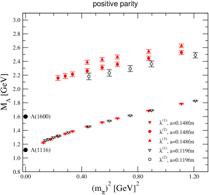
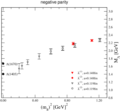
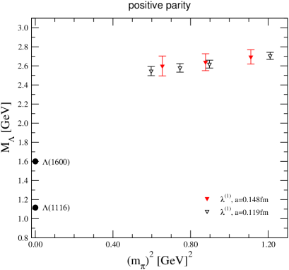
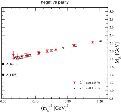
Figure 6: Ground and excited state masses obtained from our $\Lambda$ octet (upper plots) and $\Lambda$ singlet (lower plots) interpolators.

For $\Lambda$ we have considered two different kinds of interpolators; one which is a pure flavor singlet and one which has mainly overlap with a flavor octet.

For the flavor octet $\Lambda$ we obtain results which are similar to the results of the other flavor octet baryons. Even the same combination of sources used for N, $\Sigma$ and $\Xi$ turns out to be the optimal one also for the $\Lambda$ octet channel.

For the flavor singlet $\Lambda$ we are mainly interested in the ground state in both parity channels. We have therefore used only a single interpolator, the one where all quarks are smeared narrowly (choosing a different smearing combination does not change the results).

The interesting observation is that while the negative parity flavor-singlet state extrapolates to the mass which is essentially higher than $\Lambda(1405)$, which is consistent with previous quenched lattice results, the flavor-octet negative parity ground state signal is consistent with the $\Lambda(1405)$. Within the simple quark model picture the negative parity pair $1/2^{-},\Lambda(1405)-3/2^{-},\Lambda(1520)$ is a flavor-singlet. However, starting from the early Dalitz’ work it is also understood that at least a significant part of $\Lambda(1405)$ could be due to $\overline{K}N$ physics D . The $\overline{K}N$ bound state system can couple to the flavor-octet interpolator and our results hint at the $\overline{K}N$ nature of $\Lambda(1405)$. It would be very interesting to study the $3/2^{-},\Lambda(1520)$ resonance and to see whether it is a flavor-singlet or flavor-octet state.

III.5 $\Delta^{\frac{3}{2}}$ and $\Omega^{\frac{3}{2}}$

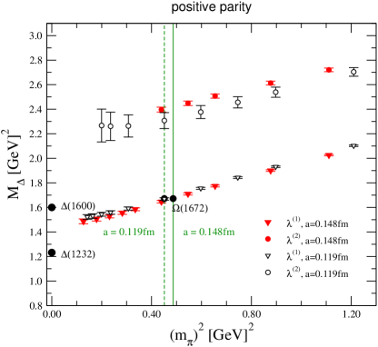
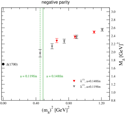
Figure 7: $\Delta$ masses versus $M_{\pi}^{2}$. The vertical lines mark the values of $M_{\pi}^{2}$ corresponding to the physical strange quark mass.

As already discussed in the previous section, our interpolators for $\Delta^{\frac{3}{2}}$ have to be spin projected to obtain correlators of states with definite quantum numbers. After the projection we are left with a set of 8 interpolators which differ only in the smearing combination of the quarks. From these we have chosen different subsets and found that the dependence on the chosen subset is only marginal. In the end, we decided to use the combinations $n(nn)$, $w(nn)$, $n(nw)$, $w(nw)$, $n(ww)$, $w(ww)$ for both parity channels.

In Fig. 7, we present the results for the $\Delta^{\frac{3}{2}}$ and $\Omega^{\frac{3}{2}}$ masses. The positive parity states are shown in the left plot, the right plot is for negative parity. The vertical lines in both plots mark the values of $m_{\pi}^{2}$ corresponding to the physical strange quark mass, which has been determined from a fit to the K-meson mass in a separate calculation on the two lattices. At these values of the pion mass we extract the masses for the $\Omega^{\frac{3}{2}}$ resonance from our results for the $\Delta^{\frac{3}{2}}$. It is remarkable that the ground state $\Omega^{\frac{3}{2}}$ lies right on top of the experimental value.

The results for the positive parity ground states of $\Delta^{\frac{3}{2}}$ show significant discrepancies with the experimental results. However, this is not unexpected and has already been observed by other groups excitedspectro3 . The Roper-like state, $\Delta(1600)$, is not reproduced either. In both cases the most probable explanation would be a lack of the proper chiral dynamics in quenched QCD. Given the fact that the $\Omega$ ground state is perfectly reproduced, one concludes that this missing chiral dynamics becomes especially important at the quark masses below the strange quark mass.

On the negative parity side we could only reliably fit the ground state and only on the fine lattice do our data reach the strange quark mass such that the mass of the negative parity $\Omega^{\frac{3}{2}}$ can be determined. Extrapolation to the physical limit is consistent with $\Delta(1700)$.

III.6 Chiral extrapolations for the fine lattice

Where the data are sufficient, we perform a chiral extrapolation of our results. For excited states the form of the chiral extrapolation is not known from chiral perturbation theory and we extrapolate linearly in $m_{\pi}^{2}$. Since in this paper the focus is on the excited states, the extrapolation for the ground states is also kept simple – we use second order polynomials in $m_{\pi}$ there, which is the structure of the leading terms in quenched chiral perturbation theory quenchchpt . Since for some of the states we still observe cutoff effects, we extrapolated only the data from the finer lattice.

For positive parity the results of the chiral extrapolation are presented in the left plot of Fig. 8. We remark, that the numbers for the $\Omega$ are obtained by an interpolation to the strange quark mass. While the ground states come out reasonably well for a quenched calculation, the results for the excited states are systematically 20 % - 25% above the experimental numbers (where known). The most likely explanation is that quenching removes some important piece of chiral physics, which is actually responsible for the proper mass of excited positive parity states. Significant finite volume effects cannot be ruled out either.

For negative parity states (right plot of Fig. 8) the results are compatible with the experimental numbers (where known), although the statistical errors are larger. Also here we cannot exclude that cutoff effects push our numbers up a little bit, but from the comparison of the results on our two lattices we estimate that this effect is not larger than the statistical error. Again the result for $\Omega$ is obtained from an interpolation to the strange quark mass. One may expect that quenching effects are essentially smaller for the negative parity channel states than for the positive parity excited states. This is expected a-priori, since all low-lying negative parity states have the mixed flavor-spin symmetry [21]_FS and hence are affected by the chiral dynamics only slightly (except for the $\Lambda(1405)$ ) GR .

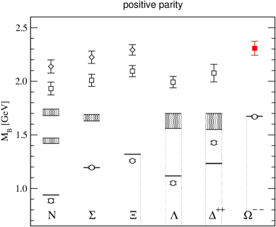
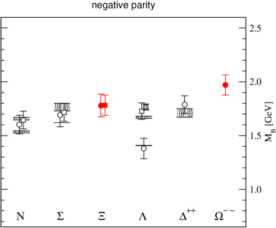
Figure 8: Chiral extrapolation of our results. The left plot is for positive parity, the right for negative parity. The horizontal bars represent the experimental numbers (where known), indicating also the error. For our results we use circles for ground states, squares and diamonds for the first and second excited states respectively. The shaded square symbol for the excited $\Lambda$ represents the chiral limit of the data from the singlet interpolator. Filled symbols are used for those states where no corresponding state is listed in the particle data book.

IV Summary

In this article we presented a quenched spectroscopy calculation of excited baryons using the variational method. We use interpolators with different Dirac structures. Furthermore each quark can either have a narrow or a wide source such that the states can have nodes in their spatial wave function.

For the positive parity baryons we find that the ground state masses are compatible with the experimental numbers, while for the excited states the masses are systematically 20% - 25% above the experimental numbers. We believe that the failure to reproduce the masses of the positive parity excited baryons is indeed mainly due to quenching where a significant part of chiral physics is missing. Large finite volume effects cannot be excluded either.

For negative parity, we find that our masses are in reasonable agreement with the experimental numbers, although here our statistical errors are larger and a further lowering of our results for a lattice with a higher cutoff cannot be excluded.

In some of the channels we analyze, the corresponding baryons are not yet classified pdg . For four of these channels we believe that our data are strong enough to quote the final results as a prediction: The first excited positive parity $\Omega$ state, the negative parity $\Omega$ ground state, and the ground and first excited negative parity $\Xi$ states.

The two $\Omega$ states are included in this list since at the strange quark mass the chiral dynamics is less important and also our results do not need to be extrapolated to the chiral limit. Concerning the two negative parity $\Xi$ states we believe that the good results of the structurally very similar negative parity nucleons and $\Sigma$ baryons justify the prediction of the mass of the negative parity ground and first excited state in the $\Xi$ channel. Our final numbers for the masses of the four states are listed in Table 3.

state	Mass [MeV]
$\Omega$, positive parity, first excited state	2300(70)
$\Omega$, negative parity, ground state	1970(90)
$\Xi$, negative parity, ground state	1780(90)
$\Xi$, negative parity, first excited state	1780(110)

Table 3: Collection of our final results for some states not classified by the Particle Data Group pdg .

- (1) N. Mathur et al., Phys. Lett. B 605, 137 (2005); F. X. Lee et al., Nucl. Phys. Proc. Suppl. 119, 296 (2003).
- (2) S. Sasaki, Prog. Theor. Phys. Suppl. 151, 143 (2003).
- (3) S. Sasaki, T. Blum and S. Ohta, Phys. Rev. D65, 074503 (2002).
- (4) D. Brömmel et al. [Bern-Graz-Regensburg Collaboration], Phys. Rev. D 69, 094513 (2004); Nucl. Phys. Proc. Suppl. 129, 251 (2004).
- (5) T. Burch et al. [Bern-Graz-Regensburg Collaboration], Phys. Rev. D 70, 054502 (2004); Nucl. Phys. Proc. Suppl. 140, 284 (2005); Nucl. Phys. A 755, 481 (2005); PoS LAT2005, 075 (2005).
- (6) K. Sasaki, S. Sasaki and T. Hatsuda, Phys. Lett. B 623, 208 (2005); K. Sasaki and S. Sasaki, PoS LAT2005, 060 (2005); S. Sasaki, K. Sasaki, T. Hatsuda and M. Asakawa, Nucl. Phys. Proc. Suppl. 129, 212 (2004); Nucl. Phys. Proc. Suppl. 119, 302 (2003);
- (7) J. M. Zanotti et al., Phys. Rev. D 68, 054506 (2003); W. Melnitchouk et al., Phys. Rev. D 67, 114506 (2003); Nucl. Phys. Proc. Suppl. 109A, 96 (2002); F. X. Lee et al., Nucl. Phys. Proc. Suppl. 106, 248 (2002); F. X. Lee and D. B. Leinweber, Nucl. Phys. Proc. Suppl. 73, 258 (1999).
- (8) K. J. Juge et al., arXiv:hep-lat/0601029; S. Basak et al. [Lattice Hadron Physics Collaboration (LHPC)], Phys. Rev. D 72, 074501 (2005); Phys. Rev. D 72, 094506 (2005); arXiv:hep-lat/0601034.
- (9) D. Guadagnoli, M. Papinutto and S. Simula, Phys. Lett. B 604, 74 (2004).
- (10) T. Burch et al. [Bern-Graz-Regensburg Collaboration], arXiv:hep-lat/0601026; PoS LAT2005, 097 (2005).
- (11) G.P. Lepage, Nucl. Phys. (Proc. Suppl.) 106, 12 (2002).
- (12) M. Asakawa, T. Hatsuda and Y. Nakahara, Prog. Part. Nucl. Phys. 46, 459 (2001).
- (13) C. Michael, Nucl. Phys. B 259, 58 (1985).
- (14) M. Lüscher and U. Wolff, Nucl. Phys. B 339, 222 (1990).
- (15) S. Güsken, et al., Phys. Lett. B 227, 266 (1989); C. Best et al., Phys. Rev. D 56, 2743 (1997).
- (16) T. Burch, C. Gattringer, L.Y. Glozman, C. Hagen and C.B. Lang, Phys. Rev. D 73, 017502 (2006).
- (17) M. Lüscher and P. Weisz, Commun. Math. Phys. 97, 59 (1985), Err.: 98, 433 (1985); G. Curci, P. Menotti and G. Paffuti, Phys. Lett. B 130, 205 (1983), Err.: 135, 516 (1984).
- (18) C. Gattringer, R. Hoffmann and S. Schaefer, Phys. Rev. D 65, 094503 (2002).
- (19) C. Gattringer, Phys. Rev. D 63, 114501 (2001); C. Gattringer, I. Hip and C. B. Lang, Nucl. Phys. B 597, 451 (2001).
- (20) P.H. Ginsparg and K.G. Wilson, Phys. Rev. D 25, 2649 (1982).
- (21) C. Gattringer et al. [Bern-Graz-Regensburg Collaboration], Nucl. Phys. B 677, 3 (2004); Nucl. Phys. Proc. Suppl. 119, 796 (2003); C. Gattringer, Nucl. Phys. Proc. Suppl. 119, 122 (2003).
- (22) L. Ya. Glozman and D. O. Riska, Phys. Rep. 268, 263 (1996); L. Ya. Glozman, W. Plessas, K. Varga, R. Wagenbrunn, Phys. Rev. D 58, 094030 (1998); L. Ya. Glozman, Nucl. Phys. A 663, 103 (2000).
- (23) For a review, see R. H. Dalitz (p. 748), in Review of Particle Physics, (D. E. Groom et al), Eur. Phys. J. C 15, 1 (2000).
- (24) J.N. Labrenz and S.R. Sharpe, Phys. Rev. D 54, 4595 (1996).
- (25) S. Eidelman et al. (Review of Particle Physics), Phys. Lett. B 592, 1 (2004).