A strategy for implementing non-perturbative renormalisation of heavy-light four-quark operators in the static approximation

Abstract:

We discuss the renormalisation properties of the complete set of $\Delta{B}=2$ four-quark operators with the heavy quark treated in the static approximation. We elucidate the rôle of heavy quark symmetry and other symmetry transformations in constraining their mixing under renormalisation. By employing the Schrödinger functional, a set of non-perturbative renormalisation conditions can be defined in terms of suitable correlation functions. As a first step in a fully non-perturbative determination of the scale-dependent renormalisation factors, we evaluate these conditions in lattice perturbation theory at one loop. Thereby we verify the expected mixing patterns and determine the anomalous dimensions of the operators at NLO in the Schrödinger functional scheme. Finally, by employing twisted-mass QCD it is shown how finite subtractions arising from explicit chiral symmetry breaking can be avoided completely.

1 Introduction

The oscillations among pairs of neutral $B$-mesons provide crucial information for pinning down the elements of the Cabibbo-Kobayashi-Maskawa (CKM) Matrix that are associated with the top quark. Owing to the absence of flavour-changing neutral currents in the Standard Model, these oscillations are described by box diagrams, in which the flavour change is brought about through the intermediate propagation of a virtual top quark. By integrating out the $W$-boson, the box diagram is replaced by an effective point-like interaction vertex associated with the left-handed $\Delta{B}=2$ four-quark operator

$${\cal O}_{\rm LL}(x)=\bar{b}(x)\gamma_{\mu}^{L}\psi_{\ell}(x)\ \bar{b}(x)\gamma_{\mu}^{L}\psi_{\ell}(x)\ ,$$ (1)

where $\gamma_{\mu}^{L}=\gamma_{\mu}(\mathds{1}-\gamma_{5})$, and the flavour label $\ell$ denotes either a $d$ or an $s$ quark. The matrix elements of ${\cal O}_{\rm LL}$ between $B$-meson states are commonly parameterised in terms of the $B$-parameters $B_{B}$ and $B_{B_{s}}$, for instance

$$\langle\bar{B}^{0}|{\cal O}_{\rm LL}|B^{0}\rangle=\frac{8}{3}m_{B}^{2}f_{B}^{2}B_{B}\ ,$$ (2)

for $\ell=d$. The operator ${\cal O}_{\rm LL}$ can be decomposed into parity-even and parity-odd components ${\cal O}_{\rm VV+AA}$ and ${\cal O}_{\rm VA+AV}$. In the Standard Model only the parity-even part ${\cal O}_{\rm VV+AA}$ makes a contribution to $B$-meson mixing. The $B$-parameters encode the long-distance effects of the strong interaction and must be determined in a non-perturbative approach such as lattice QCD. Indeed, various lattice estimates of $B_{B}$ and $B_{B_{s}}$ have been published by several authors in recent years [1, 2, 3, 4, 5, 6, 7, 8, 9, 10, 11, 12].
It is well known that relativistic $b$-quarks cannot be simulated directly for currently accessible lattice spacings. Several formalisms for treating $b$-quarks on the lattice, based on Heavy Quark Effective Theory (HQET) [13, 14], non-relativistic QCD [15], on-shell improvement for relativistic quarks [16, 17], as well as finite-size scaling techniques [18], have been developed and applied. Obviously, some, if not all, of these approaches imply certain approximations or assumptions whose validity and intrinsic accuracy must be investigated.
In order to yield useful phenomenological information, operators like ${\cal O}_{\rm LL}$ must be renormalised. If the regulator breaks chiral symmetry, as is the case for Wilson fermions, the renormalisation of ${\cal O}_{\rm LL}$, which has a particular chiral structure, is complicated by the fact that it undergoes mixing with operators of different chiralities. Therefore, in addition to an overall logarithmically divergent, multiplicative renormalisation factor, one must also determine finite subtraction coefficients.
The analogous case of $K^{0}-\bar{K}^{0}$ mixing, in which all fields that appear in the corresponding four-quark operator are treated relativistically, has been studied in ref. [19]. There the renormalisation and mixing patterns of a general set of four-quark operators were classified according to their transformation properties under certain symmetries. In particular, it was shown how the mixing due to explicit chiral symmetry breaking implied by the Wilson term could be isolated and absorbed into mixing coefficients. Another important result of [19] was the observation that the parity-odd component ${\cal O}_{\rm VA+AV}$ is protected against mixing by discrete symmetries.
In this paper we adopt a similar strategy to extend the analysis of ref. [19] to the case where the $b$-quark is treated at leading order in HQET, i.e. in the static approximation. In particular, we show how the heavy quark spin symmetry, in conjunction with transformation properties under spatial rotations, as well as discrete symmetries like parity and time reversal can be used to constrain the renormalisation patterns of a general set of static-light four-quark operators. One key result is that it is possible to find a basis of parity-odd operators that renormalise purely multiplicatively. This allows to devise a strategy aimed at a non-perturbative determination of the renormalisation factors required for the calculation of $B$-parameters, without the need to determine finite subtractions.
To this end we use twisted mass QCD (tmQCD) [20] as a discretisation for the light quark fields, which allows us to map parity-even operators to parity-odd ones. By employing the Schrödinger functional (SF) [21], the anomalous dimension of the latter can then be determined non-perturbatively in complete analogy to the case of $K^{0}-\bar{K}^{0}$ mixing studied previously in [22]. Thus, in order to reconstruct the phenomenologically relevant matrix element of ${\cal O}_{\rm LL}$, one only needs to determine the renormalisation properties of multiplicatively renormalisable operators, even in regularisations that break chiral symmetry explicitely.
In addition to explaining how the renormalisation properties of static-light four-quark operators can be constrained, another purpose of this paper is to identify – in the spirit of [23] – suitable finite-volume renormalisation schemes based on the SF, to be used in a forthcoming non-perturbative calculation. To this end we have computed the anomalous dimension in perturbation theory at NLO for the complete basis of four-quark operators in several SF schemes.
Of course, the complicated mixing patterns one is confronted with when using Wilson fermions can be avoided by using discretisations for the light quarks which obey the Ginsparg-Wilson relation. First steps in this direction have been taken in ref. [24, 25]. However, in this work we show, by using symmetry properties and tmQCD, that the renormalisation of static-light four-quark operators describing $B^{0}-\bar{B}^{0}$ mixing can be studied in an equally simple framework for Wilson-type regularisations. Non-perturbative renormalisation can thus be implemented in a straightforward manner and at much reduced computational cost.
This paper is organised as follows: in section 2 we discuss how the transformation properties under various symmetries constrain the mixing patterns of static-light four-quark operators. In section 3 we formulate a set of renormalisation conditions for the operator basis within the Schrödinger functional. Section 4 describes the perturbative calculation which yields the NLO anomalous dimensions of the operators for a set of Schrödinger functional renormalisation schemes. In section 5 we discuss the use of tmQCD to compute the physical matrix elements for $B^{0}$–$\bar{B}^{0}$ mixing using multiplicatively renormalisable operators. Our conclusions are presented in section 6. Technical details regarding the use of symmetries to constrain the renormalisation pattern and the evaluation of lattice integrals are relegated to Appendices A and B, respectively. Tables listing the finite parts of renormalisation constants and the NLO anomalous dimensions can be found in Appendix C.

2 Mixing of heavy-light four-quark operators in the static approximation

In this section we study the mixing of $\Delta B=2$ heavy-light four-quark operators in which the heavy quarks are treated in the static approximation of HQET. Thus they are represented by a pair of static fields $(\psi_{h},\psi_{\bar{h}})$, propagating forward and backward in time, respectively; their dynamics is governed by the Eichten-Hill action [26]

$$S^{\rm stat}[\psi_{h},\psi_{\bar{h}}]=a^{4}\sum_{x}\left[\bar{\psi}_{h}(x)\nabla_{0}^{*}\psi_{h}(x)-\bar{\psi}_{\bar{h}}(x)\nabla_{0}\psi_{\bar{h}}(x)\right],$$ (3)

where the forward and backward covariant derivatives $\nabla_{0},\,\nabla_{0}^{*}$ are defined by

$$\nabla_{0}\psi_{\bar{h}}(x)=\frac{1}{a}\left[U_{0}(x)\psi_{\bar{h}}(x+a\hat{0})-\psi_{\bar{h}}(x)\right],$$

$$\nabla_{0}^{*}\psi_{h}(x)=\frac{1}{a}\left[\psi_{h}(x)-U_{0}(x-a\hat{0})^{-1}\psi_{h}(x-a\hat{0})\right].$$ (4)

The field $\psi_{h}$($\bar{\psi}_{h}$) can be thought of as the annihilator(creator) of a heavy quark. Similarly, $\psi_{\bar{h}}$($\bar{\psi}_{\bar{h}}$) creates(annihilates) a heavy antiquark. Each field is represented by a four-component Dirac vector, yet only half of the components play a dynamical rôle, owing to the static projection constraints

$$P_{\scriptsize+}\psi_{h}=\psi_{h}\ ,\qquad\bar{\psi}_{h}P_{\scriptsize+}=\bar{\psi}_{h}\ ,\qquad P_{\scriptsize+}=\frac{1}{2}(\mathds{1}+\gamma_{0})\ ;$$

$$P_{\scriptsize-}\psi_{\bar{h}}=\psi_{\bar{h}}\ ,\qquad\bar{\psi}_{\bar{h}}P_{\scriptsize-}=\bar{\psi}_{\bar{h}}\ ,\qquad P_{\scriptsize-}=\frac{1}{2}(\mathds{1}-\gamma_{0})\ .$$ (5)

Instead of the link variables that appear in eq. (4) one can consider more general definitions of the parallel transporter which enters the covariant derivative. A set of alternative discretisations was studied in [27], where it was found that adequate choices of parallel transporter lead to much improved signal-to-noise ratios in actual simulations.

The light (relativistic) quarks are instead taken to be Wilson fermions, using either the plain Wilson action or its $\mbox{O}(a)$ improved version with a Sheikholeslami-Wohlert term [28]. The explicit chiral symmetry breaking induced by the Wilson term causes the mixing of operator of different naive chirality even in the chiral limit.

We consider a complete basis of $\Delta B=2$ heavy-light four-quark operators which, for the sake of definiteness, we chose to contain two static fields $\bar{\psi}_{h}$ and $\bar{\psi}_{\bar{h}}$ while, in the light sector, we consider massless fermions with two distinct flavours $\psi_{1}$ and $\psi_{2}$. We introduce a generic $\Delta B=2$ operator via

$${\cal O}^{\pm}_{\Gamma_{1}\Gamma_{2}}=\dfrac{1}{2}\left[(\bar{\psi}_{h}\Gamma_{1}\psi_{1})(\bar{\psi}_{\bar{h}}\Gamma_{2}\psi_{2})\pm(\bar{\psi}_{h}\Gamma_{1}\psi_{2})(\bar{\psi}_{\bar{h}}\Gamma_{2}\psi_{1})\right]\ ,$$ (6)

where $\Gamma_{1,2}$ are Dirac matrices, and we adopt the notation

$${\cal O}^{\pm}_{\Gamma_{1}\Gamma_{2}\ \pm\ \Gamma_{3}\Gamma_{4}}\equiv{\cal O}^{\pm}_{\Gamma_{1}\Gamma_{2}}\pm{\cal O}^{\pm}_{\Gamma_{3}\Gamma_{4}}\ .$$ (7)

The complete basis of Lorentz invariant operators is given by the set of 16 operators

$$\hbox{parity-even:~{}~{}}Q_{1}^{\pm} ={\cal O}^{\pm}_{\rm VV+AA}\ ,\qquad\hbox{parity-odd:~{}~{}} {{\cal Q}}_{1}^{\pm} ={\cal O}^{\pm}_{\rm VA+AV}\ ,$$

$$Q_{2}^{\pm} ={\cal O}^{\pm}_{\rm SS+PP}\ , {{\cal Q}}_{2}^{\pm} ={\cal O}^{\pm}_{\rm SP+PS}\,$$

$$Q_{3}^{\pm} ={\cal O}^{\pm}_{\rm VV-AA}\ , {{\cal Q}}_{3}^{\pm} ={\cal O}^{\pm}_{\rm VA-AV}\ ,$$

$$Q_{4}^{\pm} ={\cal O}^{\pm}_{\rm SS-PP}\ , {{\cal Q}}_{4}^{\pm} ={\cal O}^{\pm}_{\rm SP-PS}\ ,$$ (8)

which we have grouped according to their transformation properties under parity. Here ${\rm V}=\gamma_{\mu}$, ${\rm A}=\gamma_{\mu}\gamma_{5}$, $S=\mathds{1}$, ${\rm P}=\gamma_{5}$, and an implicit summation over pairs of Lorentz indices is understood. We incidentally remind the reader that tensor structures like $T=\sigma_{\mu\nu}$ or $\tilde{T}=\sigma_{\mu\nu}\gamma_{5}$ produce redundant operators in the static limit, due the projection constraints (2).

The description of $\Delta{B}=2$ transitions in terms of the static approximation of HQET implies that the operator ${\cal{O}}_{\rm LL}$ of eq. (1) is related in some particular way to the operators listed in eq. (2). Owing to the heavy-quark spin symmetry, one finds that ${\cal{O}}_{\rm LL}$ must be matched to a linear combination of ${\cal{O}}^{+}_{\rm VV+AA}$ and ${\cal{O}}^{+}_{\rm SS+PP}$ [29], and thus those two operators are of particular interest to the study of $B^{0}-\bar{B}^{0}$ mixing.

The operator basis in eq. (2) renormalises, in full generality, via a $16\times 16$ matrix ${\mathbb{Z}}$, the form of which can be constrained through symmetry arguments. A systematic method to carry out this analysis is given by the following prescription:

• Construct the matrices $\Phi_{k}$ that implement, at the level of the operator basis, a maximal set of independent symmetry transformations that leave the action invariant.

• Impose the constraints

  $${\mathbb{Z}}=\Phi_{k}{\mathbb{Z}}\Phi_{k}^{-1},\ \forall k.$$ (9)

  The solution ${\mathbb{Z}}$ to this system of equations displays the constrained form of the renormalisation matrix.

In most cases the constraint imposed by a given symmetry on the renormalisation matrix $\mathds{Z}$ can be easily found out, while in a few cases (namely heavy quark spin symmetry and $H(3)$ spatial rotations) an explicit construction of the corresponding $\Phi_{k}$ matrices is required. We leave the explanation of this procedure to Appendix A and we present here the list of symmetries that have been used and their effect in constraining the matrix $\mathds{Z}$. Flavour exchange symmetry ${\cal S}$. ${\cal S}$ exchanges the two relativistic flavours $\psi_{1}$ and $\psi_{2}$. Operators with superscript $\pm$ are eigenvectors of $\Phi_{\cal S}$ with eigenvalues $\pm 1$ respectively. ${\cal S}$ thus prevents the mixing between the $+$ and $-$ sectors. This reduces the renormalisation matrix ${\mathbb{Z}}$ to a block-diagonal form, with two $8\times 8$ blocks. Parity. Mixing among operators with opposite parity is excluded, and the renormalisation matrix ${\mathbb{Z}}$ is reduced to a block-diagonal form, where four $4\times 4$ blocks describe the mixing of the parity-even and parity-odd operators among themselves. Chiral symmetry. It is used in the same way as in ref. [19]. In the chiral limit, the continuum relativistic quark action is invariant under the finite axial transformation:

$$\psi_{k}\rightarrow i\gamma_{5}\psi_{k}\,;\qquad\bar{\psi}_{k}\rightarrow i\bar{\psi}_{k}\gamma_{5}\ .$$ (10)

Under this transformation we obtain:

$$Q^{\pm}_{1}\rightarrow-Q^{\pm}_{1}~{}, {\cal Q}^{\pm}_{1}\rightarrow-{\cal Q}^{\pm}_{1}~{},$$

$$Q^{\pm}_{2}\rightarrow-Q^{\pm}_{2}~{}, {\cal Q}^{\pm}_{2}\rightarrow-{\cal Q}^{\pm}_{2}~{},$$

$$Q^{\pm}_{3}\rightarrow\phantom{-}Q^{\pm}_{3}~{}, {\cal Q}^{\pm}_{3}\rightarrow\phantom{-}{\cal Q}^{\pm}_{3}~{},$$

$$Q^{\pm}_{4}\rightarrow\phantom{-}Q^{\pm}_{4}~{}, {\cal Q}^{\pm}_{4}\rightarrow\phantom{-}{\cal Q}^{\pm}_{4}~{}.$$ (11)

From this one sees that, were chirality respected by the regulator, $Q^{\pm}_{1}$ would mix only with $Q^{\pm}_{2}$, and $Q^{\pm}_{3}$ only with $Q^{\pm}_{4}$ (and similarly in the parity-odd sector). This is not the case with a Wilson regularisation, for which the structure of chiral multiplets must be restored by combining operators with different naive chiralities [30]. The restoration of chiral properties is achieved by introducing the mixing matrices $\Delta^{\pm},\mbox{\textcyr{D}}^{\pm}$. Once the subtracted operators $\tilde{Q}^{\pm}=(\mathds{1}+\Delta^{\pm})Q^{\pm}$ and $\tilde{\cal Q}^{\pm}=(\mathds{1}+\mbox{\textcyr{D}}^{\pm}){\cal Q}^{\pm}$ with the correct chiral properties have been constructed, they will mix like in the continuum with renormalisation matrices $Z^{\pm},{\cal Z}^{\pm}$. We choose the matrices $Z^{\pm},{\cal Z}^{\pm},\Delta^{\pm},\mbox{\textcyr{D}}^{\pm}$ such that:

$$\left(\begin{array}[]{c}Q_{1}^{\pm}\\ Q_{2}^{\pm}\\ Q_{3}^{\pm}\\ Q_{4}^{\pm}\end{array}\right)_{\rm R}=\left(\begin{array}[]{cccc}Z_{11}^{\pm}&Z_{12}^{\pm}&0&0\\ Z_{21}^{\pm}&Z_{22}^{\pm}&0&0\\ 0&0&Z_{33}^{\pm}&Z_{34}^{\pm}\\ 0&0&Z_{43}^{\pm}&Z_{44}^{\pm}\end{array}\right){\left[\mathds{1}+\left(\begin{array}[]{cccc}0&0&\Delta_{13}^{\pm}&\Delta_{14}^{\pm}\\ 0&0&\Delta_{23}^{\pm}&\Delta_{24}^{\pm}\\ \Delta_{31}^{\pm}&\Delta_{32}^{\pm}&0&0\\ \Delta_{41}^{\pm}&\Delta_{42}^{\pm}&0&0\end{array}\right)\right]}\left(\begin{array}[]{c}Q_{1}^{\pm}\\ Q_{2}^{\pm}\\ Q_{3}^{\pm}\\ Q_{4}^{\pm}\end{array}\right),$$ (28)

and

$$\left(\begin{array}[]{c}{\cal Q}_{1}^{\pm}\\ {\cal Q}_{2}^{\pm}\\ {\cal Q}_{3}^{\pm}\\ {\cal Q}_{4}^{\pm}\end{array}\right)_{\rm R}=\left(\begin{array}[]{cccc}{\cal Z}_{11}^{\pm}&{\cal Z}_{12}^{\pm}&0&0\\ {\cal Z}_{21}^{\pm}&{\cal Z}_{22}^{\pm}&0&0\\ 0&0&{\cal Z}_{33}^{\pm}&{\cal Z}_{34}^{\pm}\\ 0&0&{\cal Z}_{43}^{\pm}&{\cal Z}_{44}^{\pm}\end{array}\right){\left[\mathds{1}+\left(\begin{array}[]{cccc}0&0&\mbox{\textcyr{D}}_{13}^{\pm}&\mbox{\textcyr{D}}_{14}^{\pm}\\ 0&0&\mbox{\textcyr{D}}_{23}^{\pm}&\mbox{\textcyr{D}}_{24}^{\pm}\\ \mbox{\textcyr{D}}_{31}^{\pm}&\mbox{\textcyr{D}}_{32}^{\pm}&0&0\\ \mbox{\textcyr{D}}_{41}^{\pm}&\mbox{\textcyr{D}}_{42}^{\pm}&0&0\end{array}\right)\right]}\left(\begin{array}[]{c}{\cal Q}_{1}^{\pm}\\ {\cal Q}_{2}^{\pm}\\ {\cal Q}_{3}^{\pm}\\ {\cal Q}_{4}^{\pm}\end{array}\right).$$ (45)

This choice is convenient because it is easy to show (for instance by using Ward identities) that $\Delta^{\pm},\ \mbox{\textcyr{D}}^{\pm}$ and the product ${\cal Z}^{\pm}(Z^{\pm})^{-1}$ all depend only on the bare coupling $g_{0}$, while $Z^{\pm}$ and ${\cal Z}^{\pm}$ alone contain the continuum-like dependence on the renormalisation scale. Heavy quark spin symmetry and $H(3)$ spatial rotations. Further constraints can be obtained from the heavy quark spin symmetry and cubic rotations. The procedure is slightly involved and we leave its description to Appendix A. It applies identically to both parity-even and parity-odd sectors, and below we provide the expressions for the latter — results for the parity-even sector are obtained by simply replacing the symbols ${\cal Q},{\cal Z},\mbox{\textcyr{D}}$ with $Q,Z,\Delta$. After imposing the constraints ${\mathbb{Z}}=\Phi_{k}{\mathbb{Z}}\Phi_{k}^{-1}$ one finds that it is possible to rotate (2) into a new basis

$$({\cal Q}^{\prime\pm}_{1},{\cal Q}^{\prime\pm}_{2},{\cal Q}^{\prime\pm}_{3},{\cal Q}^{\prime\pm}_{4})^{T}=({\cal Q}^{\pm}_{1},{\cal Q}^{\pm}_{1}+4{\cal Q}^{\pm}_{2},{\cal Q}^{\pm}_{3}+2{\cal Q}^{\pm}_{4},{\cal Q}^{\pm}_{3}-2{\cal Q}^{\pm}_{4})^{T},$$ (46)

in which the scale-dependent mixing is completely disentangled (even though some scale-independent mixing remains):

$$\left(\begin{array}[]{c}{\cal Q}_{1}^{\prime\pm}\\ {\cal Q}_{2}^{\prime\pm}\\ {\cal Q}_{3}^{\prime\pm}\\ {\cal Q}_{4}^{\prime\pm}\end{array}\right)_{\rm R}=\left(\begin{array}[]{cccc}{\cal Z}_{1}^{\prime\pm}&0&0&0\\ 0&{\cal Z}_{2}^{\prime\pm}&0&0\\ 0&0&{\cal Z}_{3}^{\prime\pm}&0\\ 0&0&0&{\cal Z}_{4}^{\prime\pm}\end{array}\right){\left[\mathds{1}+\left(\begin{array}[]{cccc}0&0&\mbox{\textcyr{D}}_{1}^{\prime\pm}&0\\ 0&0&0&\mbox{\textcyr{D}}_{2}^{\prime\pm}\\ \mbox{\textcyr{D}}_{3}^{\prime\pm}&0&0&0\\ 0&\mbox{\textcyr{D}}_{4}^{\prime\pm}&0&0\end{array}\right)\right]}\left(\begin{array}[]{c}{\cal Q}_{1}^{\prime\pm}\\ {\cal Q}_{1}^{\prime\pm}\\ {\cal Q}_{3}^{\prime\pm}\\ {\cal Q}_{3}^{\prime\pm}\end{array}\right).$$ (63)

Time reversal. Up to this point, the renormalisation mixing of the parity-even and parity-odd sectors has the same matrix structure. We now consider the effect of a time reversal transformation of both the static and relativistic quark fields. To that purpose, it is convenient to rewrite (6) in the form

$${\cal O}^{\pm}_{\Gamma_{1}\Gamma_{2}}=\frac{1}{2}\left[\left(\bar{\Psi}P_{\scriptsize+}\Gamma_{1}\psi_{1}\right)\left(\bar{\Psi}P_{\scriptsize-}\Gamma_{2}\psi_{2}\right)\pm\left(\bar{\Psi}P_{\scriptsize-}\Gamma_{1}\psi_{2}\right)\left(\bar{\Psi}P_{\scriptsize+}\Gamma_{2}\psi_{1}\right)\right]\ ,$$ (64)

with

$$\Psi=\psi_{h}+\psi_{\bar{h}}\ ,\qquad\bar{\Psi}=\bar{\psi}_{h}+\bar{\psi}_{\bar{h}}\ .$$ (65)

It is then easy to apply the time reversal transformation

$$\begin{split}\bar{\Psi}(x)&\to\bar{\Psi}(x^{\tau})\gamma_{5}\gamma_{0},\\ \psi_{k}(x)&\to\gamma_{0}\gamma_{5}\psi_{k}(x^{\tau}),\quad k=1,2\end{split}$$ (66)

where $(x_{0},{\bf x})^{\tau}=(-x_{0},{\bf x})$.

The transformation rules for the operators (apart from the $\tau$ reflection of the space-time coordinates) are easily found to be

$$Q_{1}^{\pm}\to\pm Q_{1}^{\pm} {\cal Q}_{1}^{\pm}\to\mp{\cal Q}_{1}^{\pm}\ ,$$

$$Q_{2}^{\pm}\to\pm Q_{2}^{\pm} {\cal Q}_{2}^{\pm}\to\mp{\cal Q}_{2}^{\pm}\ ,$$

$$Q_{3}^{\pm}\to\pm Q_{3}^{\pm} {\cal Q}_{3}^{\pm}\to\pm{\cal Q}_{3}^{\pm}\ ,$$

$$Q_{4}^{\pm}\to\pm Q_{4}^{\pm} {\cal Q}_{4}^{\pm}\to\pm{\cal Q}_{4}^{\pm}$$ (67)

and identical ones for the $(Q^{\prime},{\cal Q}^{\prime})$ basis. It is then clear that no new constraints arise for the parity-even operators and for ${\cal Z}^{\prime\pm}$, while the invariance of the scale independent mixing under time reversal immediately yields

$$\mbox{\textcyr{D}}^{\prime\pm}=0.$$ (68)

This proves the purely multiplicative renormalisability of the operator basis (46). As a note of reference, we would like to point out that the absence of mixing is already manifest at the one-loop perturbative level in eqs. (20)–(23) of [6]: it is enough to project both sides onto parity eigenstates and change to the basis in eq. (46) to find that mixing in the parity-odd sector is absent at one loop.

Finally, we can rotate back to the standard basis (2), obtaining the following form for the renormalisation matrices:

$$Z^{\pm} =\left(\begin{array}[]{cccc}Z^{\prime\pm}_{1}&0&0&0\\ -\frac{1}{4}(Z^{\prime\pm}_{1}-Z^{\prime\pm}_{2})&Z^{\prime\pm}_{2}&0&0\\ 0&0&\frac{1}{2}(Z^{\prime\pm}_{3}+Z^{\prime\pm}_{4})&Z^{\prime\pm}_{3}-Z^{\prime\pm}_{4}\\ 0&0&\frac{1}{4}(Z^{\prime\pm}_{3}-Z^{\prime\pm}_{4})&\frac{1}{2}(Z^{\prime\pm}_{3}+Z^{\prime\pm}_{4})\end{array}\right)\ ,$$ (73)

$$\Delta^{\pm} =\left(\begin{array}[]{cccc}0&0&\Delta^{\prime\pm}_{1}&2\Delta^{\prime\pm}_{1}\\ 0&0&-\frac{1}{4}(\Delta^{\prime\pm}_{1}-\Delta^{\prime\pm}_{2})&-\frac{1}{2}(\Delta^{\prime\pm}_{1}+\Delta^{\prime\pm}_{2})\\ \frac{1}{2}(\Delta^{\prime\pm}_{3}+\Delta^{\prime\pm}_{4})&2\Delta^{\prime\pm}_{4}&0&0\\ \frac{1}{4}(\Delta^{\prime\pm}_{3}-\Delta^{\prime\pm}_{4})&-\Delta^{\prime\pm}_{4}&0&0\end{array}\right)\ ,$$ (78)

$${\cal Z}^{\pm} =\left(\begin{array}[]{cccc}{\cal Z}^{\prime\pm}_{1}&0&0&0\\ -\frac{1}{4}({\cal Z}^{\prime\pm}_{1}-{\cal Z}^{\prime\pm}_{2})&{\cal Z}^{\prime\pm}_{2}&0&0\\ 0&0&\frac{1}{2}({\cal Z}^{\prime\pm}_{3}+{\cal Z}^{\prime\pm}_{4})&{\cal Z}^{\prime\pm}_{3}-{\cal Z}^{\prime\pm}_{4}\\ 0&0&\frac{1}{4}({\cal Z}^{\prime\pm}_{3}-{\cal Z}^{\prime\pm}_{4})&\frac{1}{2}({\cal Z}^{\prime\pm}_{3}+{\cal Z}^{\prime\pm}_{4})\end{array}\right)\ ,$$ (83)

$$\mbox{\textcyr{D}}^{\pm} =0\,.$$ (84)

For later convenience, we denote by $\Lambda$ the matrix responsible for the change of basis (46), such that ${\cal Q}_{i}^{\prime\pm}=\Lambda_{ij}{\cal Q}_{j}^{\pm}$ and $Q_{i}^{\prime\pm}=\Lambda_{ij}Q_{j}^{\pm}$. Equation (73) reproduces the result of [24].

Now we will pursue a strategy to compute the renormalisation matrices non perturbatively using Schrödinger functional techniques. For parity-even operators, the determination of the subtraction coefficients in eq. (78) can be achieved by implementing suitable axial Ward identities. However, as we will show later on, the use of tmQCD techniques allows to obtain all the $\Delta B=2$ physical amplitudes of interest in the Standard Model from matrix elements of the operators ${\cal Q}_{1}^{+},{\cal Q}_{2}^{+}$. Therefore, from now on we will concentrate exclusively on the renormalisation of ${\cal Q}_{k}^{\pm}$.

3 Renormalisation conditions in the Schrödinger functional

Having constrained their renormalisation patterns by imposing the symmetries of the theory, we now proceed to specifying suitable renormalisation conditions on the four-quark operators (46). To this end we will consider a set of correlation functions defined in the Schrödinger functional (SF) which will serve to impose the renormalisation conditions at the non-perturbative level. The SF formalism [21], which was initially developed to produce a precise determination of the running coupling [31, 32, 33], has been extended to various other phenomenological contexts. These include the study of quark masses [34, 35, 36] and decay constants [37, 38, 39], the computation of moments of structure functions [40, 41], the Kaon $B$-parameter [22, 23, 42], and the static-light axial current [43, 44]. The reader is referred to [45] for detailed explanations of the framework and the standard notation, which are not repeated here.

Our construction of the relevant SF correlators extends the one described in [23] to the static case. We start by introducing the following bilinear boundary source operators, projected to zero external momentum,

$$\Sigma_{s_{1}s_{2}}[\Gamma] =a^{6}\sum_{\mathbf{x},\mathbf{y}}\bar{\zeta}_{s_{1}}(\mathbf{x})\Gamma\zeta_{s_{2}}(\mathbf{y})\ ,$$

$$\Sigma^{\prime}_{s_{1}s_{2}}[\Gamma] =a^{6}\sum_{\mathbf{x},\mathbf{y}}\bar{\zeta}^{\prime}_{s_{1}}(\mathbf{x})\Gamma\zeta^{\prime}_{s_{2}}(\mathbf{y})\ ,$$ (85)

where $\Gamma$ is a Dirac matrix, the flavour indices $s_{1,2}$ can assume both relativistic and static values, and the fields $\zeta$ and $\zeta^{\prime}$ represent functional derivatives with respect to the fermionic boundary fields of the SF, see [45]. The choices for $\Gamma$ are limited by the boundary conditions imposed on quark fields. At the level of boundary quark and antiquark fields they imply

$$\zeta(\mathbf{x})=P_{-}\zeta(\mathbf{x})\,,~{}~{}~{}~{}~{}~{}~{}~{}~{}~{}~{}~{}\bar{\zeta}(\mathbf{x})=\bar{\zeta}(\mathbf{x})P_{+}\,,$$ (86)

with $P_{\pm}={\scriptstyle{{1\over 2}}}(\mathds{1}\pm\gamma_{0})$, and similarly for $\zeta^{\prime},\bar{\zeta}^{\prime}$. Therefore, in order to have a non-vanishing source field $\Sigma_{s_{1}s_{2}}[\Gamma]$, $\Gamma$ must anticommute with $\gamma_{0}$.

Starting from the bilinears in (3), we have to construct suitable boundary sources to probe four-quark operators. In order to define a set of non-zero correlators in the massless theory, which can then be used to impose renormalisation conditions in the chiral limit, the probe should be parity-odd. We further require it to be invariant under the group $H(3)$ of lattice rotations in three dimensions. This leads us to introduce a third “spectator” light quark and consider, as the simplest possible choice, a generalised boundary source made of three bilinears,

$${\cal W}[{\Gamma}_{1},{\Gamma}_{2},{\Gamma}_{3}] =\Sigma_{1h}[{\Gamma}_{1}]\Sigma_{23}[{\Gamma}_{2}]\Sigma^{\prime}_{3\bar{h}}[{\Gamma}_{3}]\ ,$$ (87)

two of which are localised at the boundary $x_{0}=0$, while the third lies at the other boundary, namely $x_{0}=T$. Odd parity and rotational invariance are then assured through an appropriate choice of the Dirac structures $[\Gamma_{1},\Gamma_{2},\Gamma_{3}]$, and a maximal set of corresponding probes is given by

$${\cal S}^{(1)} ={\cal W}[\gamma_{5},\gamma_{5},\gamma_{5}]\ ,$$ (88)

$${\cal S}^{(2)} =\frac{1}{6}\sum_{k,l,m=1}^{3}\varepsilon_{klm}{\cal W}[\gamma_{k},\gamma_{l},\gamma_{m}]\ ,$$ (89)

$${\cal S}^{(3)} =\frac{1}{3}\sum_{k=1}^{3}{\cal W}[\gamma_{5},\gamma_{k},\gamma_{k}]\ ,$$ (90)

$${\cal S}^{(4)} =\frac{1}{3}\sum_{k=1}^{3}{\cal W}[\gamma_{k},\gamma_{5},\gamma_{k}]\ ,$$ (91)

$${\cal S}^{(5)} =\frac{1}{3}\sum_{k=1}^{3}{\cal W}[\gamma_{k},\gamma_{k},\gamma_{5}]\ .$$ (92)

The four-quark operators can now be treated as local insertions in the bulk of the SF, and their correlators are naturally defined as

$${\cal F}^{\pm;(s)}_{k}(x_{0}) =L^{-3}\langle{\cal Q}^{\prime\pm}_{k}(x){\cal S}^{(s)}\rangle,\quad s=1,\ldots,5\ .$$ (93)

A pictorial interpretation of (93) is provided by the left diagram of Figure 1.

It has to be observed that, due to the symmetries of the static approximation for the heavy quarks, not all of the above correlation functions are independent. By using the explicit spin structure of the static propagator, some straightforward though tedious algebra leads to the constraints

Figure 1: Diagrammatic representation of correlation functions: the four-quark correlator ${\cal F}_{k}^{\pm;(s)}(x_{0})$ (left), the boundary-to-boundary static-light correlators $f_{1,hl},k_{1,hl}$ (center) and the boundary-to-boundary light-light correlators $f_{1,ll},k_{1,ll}$ (right). Euclidean time goes from left to right. The double blob indicates the four-quark operator insertion. Single lines represent relativistic quarks and double lines denote the static ones.

$${\cal F}_{1}^{\pm;(4)} =-{\cal F}_{1}^{\pm;(1)}\ ,\qquad{\cal F}_{1}^{\pm;(3)} =-{\cal F}_{1}^{\pm;(2)}\ ,$$

$${\cal F}_{2}^{\pm;(4)} =\frac{1}{3}{\cal F}_{2}^{\pm;(1)}\ ,\qquad{\cal F}_{1}^{\pm;(5)} =-{\cal F}_{1}^{\pm;(2)}\ ,$$

$${\cal F}_{3}^{\pm;(4)} =-{\cal F}_{3}^{\pm;(1)}\ ,\qquad{\cal F}_{3}^{\pm;(3)} =-{\cal F}_{3}^{\pm;(2)}\ ,$$

$${\cal F}_{4}^{\pm;(4)} =\frac{1}{3}{\cal F}_{4}^{\pm;(1)}\ ,\qquad{\cal F}_{3}^{\pm;(5)} =-{\cal F}_{3}^{\pm;(2)}\ .$$ (94)

These relations show that only 24 out of the 40 correlation functions defined in eq. (93) are independent. We stress that this result is exact; as a cross-check, later on we will find these identities to be explicitly verified at one loop in perturbation theory.

In order to isolate from eq. (93) the ultraviolet divergences that are due to the bulk operator and absorb them into a renormalisation factor, one has to address the renormalisation of the boundary fields. The ultraviolet divergences of the latter are cancelled by defining suitable ratios of correlators for which the renormalisation factors of the boundary fields drop out. To this end we introduce a set of boundary-to-boundary light-light and static-light correlators,

$$f_{1}^{hl} =-\frac{1}{2L^{6}}\langle{\cal O}^{\prime}_{1\bar{h}}[\gamma_{5}]{\cal O}_{h1}[\gamma_{5}]\rangle\ ,$$ (95)

$$f_{1}^{ll} =-\frac{1}{2L^{6}}\langle{\cal O}^{\prime}_{12}[\gamma_{5}]{\cal O}_{21}[\gamma_{5}]\rangle\ ,$$ (96)

$$k_{1}^{ll} =-\frac{1}{6L^{6}}\sum_{k=1}^{3}\langle{\cal O}^{\prime}_{12}[\gamma_{k}]{\cal O}_{21}[\gamma_{k}]\rangle\ ,$$ (97)

whose valence structure is represented as well in the middle and right diagrams of Figure 1.  A suitable combination of such correlators must comprise the same number of static and light boundary fields as (93). The simplest examples are given by the ratios

$$\frac{{\cal F}_{k}^{\pm;(s)}(x_{0})}{f_{1}^{hl}[f_{1}^{ll}]^{1/2}},\qquad\frac{{\cal F}_{k}^{\pm;(s)}(x_{0})}{f_{1}^{hl}[k_{1}^{ll}]^{1/2}},$$ (98)

involving either the correlator $f_{1}^{ll}$ or $k_{1}^{ll}$. However, it is easy to generalise these conditions by introducing an arbitrary real parameter $\alpha$. Hence, we consider the following ratios of correlation functions:

$$h_{k;\alpha}^{\pm;(s)}(x_{0}) =\frac{{\cal F}_{k}^{\pm;(s)}(x_{0})}{f_{1}^{hl}[f_{1}^{ll}]^{1/2-\alpha}[k_{1}^{ll}]^{\alpha}}\ .$$ (99)

Although there is no real a priori restriction on the value of $\alpha$, it is clear that “natural” values should lie in the interval $[0,{\scriptstyle{{1\over 2}}}]$. This freedom, together with the choice of the boundary source and the $\theta$-angle of the SF, can be used in a later stage to tune the optimal renormalisation schemes, with the aim of having small NLO coefficients in the corresponding anomalous dimensions. This is important in order to control the systematics of the perturbative matching to continuum schemes at high energy scales.

For the moment we observe that the ratios (99) are free of boundary divergences, and consequently we impose the renormalisation condition,

$${\cal Z}^{\prime\pm;(s)}_{k;\alpha}h_{k;\alpha}^{\pm;(s)}(T/2) =h_{k;\alpha}^{\pm;(s)}(T/2)|_{g_{0}=0}\ ,$$ (100)

where all the correlation functions are computed in the chiral limit. This fixes non-perturbatively the renormalisation constant ${\cal Z}^{\prime\pm;(s)}_{k;\alpha}$ at the scale $\mu=1/L$. As usual, the ${\cal Z}^{\prime}$ factors depend upon every calculational detail with the only exception of the leading log, which is universal. In order to operatively define a renormalisation scheme, a complete specification of the parameters that concur to quantify (99) is required. We briefly summarise them:

• the possible presence of a Sheikholeslami-Wohlert (SW) term in the lattice action for the light quarks;

• the choice of the gauge parallel transporter in the covariant derivatives, eq. (4), in the static action;

• the Dirac structure of the boundary source;

• the value of the angle $\theta$ entering the spatial boundary conditions of the SF;

• the value of the parameter $\alpha$ in eq. (99);

• the ratio $T/L$ between the time and the spatial extension of the SF.

The last four conditions fix the renormalisation scheme, while the first two only introduce a regularisation dependence in the renormalisation constants. We stress at this point that the running of the operators is a continuum property, i.e. it is independent of the discretisation chosen. The latter only affects the way in which the continuum limit is approached, and – in the case of the action for static quark fields – the signal-to-noise ratio in the simulations.

In this paper we consider the Wilson action (with and without SW term) for the light quarks, and the Eichten-Hill action for the static ones. As for the parameters that fix the renormalisation scheme, we will consider three values of $\theta$ (namely $\theta=0.0,~{}0.5,~{}1.0$) and two values of $\alpha$ (namely $\alpha=0.0,~{}0.5$). Furthermore, we fix $T=L$. Taken together with the possible independent choices of boundary sources, this leaves us with 12 different renormalisation schemes for the operators ${\cal Q}^{\prime\pm}_{1}$ and ${\cal Q}^{\prime\pm}_{3}$, and 24 schemes for ${\cal Q}^{\prime\pm}_{2}$ and ${\cal Q}^{\prime\pm}_{4}$. The number of independent renormalisation conditions is twice this figure, as we consider two different actions.

4 A perturbative study

We now proceed to studying the renormalisation of the operators ${\cal Q}_{1}^{+},\ldots,{\cal Q}_{4}^{+}$ at one-loop in perturbation theory. These are the operators that will enter $\Delta B=2$ effective Hamiltonians in the static limit. The purpose of this study is threefold. First, it provides an explicit check of the expected mixing pattern. Second, it will allow us to compute the NLO anomalous dimension of the operators in the SF schemes defined above; this is done via a standard one-loop matching procedure to continuum schemes where the NLO anomalous dimension is already known. Finally, we can work out lattice artefacts of the step scaling functions in one-loop perturbation theory. They can then be compared to the ones in the relativistic case discussed in [23], in order to obtain information about the expected size of discretisation effects for quantities involving static fields. In principle, the discretisation effects computed in perturbation theory could subsequently be subtracted by hand from the non-perturbative Monte Carlo data, with the aim of exerting a better control of their continuum extrapolation, as pursued in [46, 47, 22].

4.1 Scheme dependence of NLO anomalous dimensions

In order to proceed, some notation has to be fixed. The scale dependence of operator insertions in renormalised correlation functions is described by the RG equation

$$\left[\delta_{ij}\left(\mu\frac{\partial}{\partial\mu}+\beta\frac{\partial}{\partial g}+\beta_{\lambda}\lambda\frac{\partial}{\partial\lambda}+\tau m\frac{\partial}{\partial m}\right)-\gamma_{ij}^{\scriptsize+}\right]({\cal Q}^{+}_{j})_{\rm R}=0\ ,$$ (101)

where $\beta$ is the $\beta$-function for the coupling, $\tau$ is the anomalous dimension of the quark mass, and $\gamma^{+}$ is the operator anomalous dimension matrix. We have also included a term which takes into account the dependence on the gauge parameter $\lambda$ in covariant gauges, characterised by the RG function $\beta_{\lambda}$, defined as

$$\mu\frac{\partial\lambda}{\partial\mu}=\lambda\beta_{\lambda}\,.$$ (102)

This term is absent in schemes like $\overline{\rm MS}$ (irrespective of the regularisation prescription) or the SF schemes introduced in section 3, but is present e.g. in regularisation-independent (RI) schemes, which will be considered later on. If we choose to work with the operator basis in eq. (46), the matrix structure of the RG-equation simplifies, and the evolution of the various operators is determined by a set of scalar anomalous dimensions.

In what follows, we focus on mass-independent renormalisation schemes, for which the RG functions depend only upon the coupling. We take the following form for their perturbative expansions:

$$\beta(g) = -g^{3}\sum_{k=1}^{\infty}b_{k}g^{2k}\ ,\qquad\beta_{\lambda}(g) =-g^{2}\sum_{k=0}^{\infty}b_{k}^{\lambda}g^{2k}\ ,$$

$$\tau(g) = -g^{2}\sum_{k=0}^{\infty}d_{k}g^{2k}\ ,\qquad\gamma_{ij}^{+}(g) =-g^{2}\sum_{k=0}^{\infty}\gamma^{{\scriptsize+};(k)}_{ij}g^{2k}\ ,$$ (103)

with universal coefficients

$$b_{0} =\frac{1}{(4\pi)^{2}}\left\{\frac{11}{3}N-\frac{2}{3}N_{\rm f}\right\}\ ,\qquad d_{0}=\frac{1}{(4\pi)^{2}}\left\{3\frac{N^{2}-1}{N}\right\}\ ,$$

$$b_{0}^{\lambda} =\frac{1}{(4\pi)^{2}}\left\{N\left(\lambda-\frac{13}{3}\right)+\frac{4}{3}N_{\rm f}\right\}\ ,$$

$$b_{1} =\frac{1}{(4\pi)^{4}}\left\{\frac{34}{3}N^{2}-\left(\frac{13}{3}N-N^{-1}\right)N_{\rm f}\right\}\ .$$ (104)

The LO coefficient of the anomalous dimension matrix $\gamma^{+;(0)}$ is universal as well, and has been calculated in [29] for the first operator of the basis and [6] for the rest. The non-vanishing elements of the anomalous dimension matrix read

$$\gamma_{11}^{+;(0)} =-\frac{1}{(4\pi)^{2}}\left(3N-\frac{3}{N}\right)\ ,$$ (105)

$$\gamma_{21}^{+;(0)} =\frac{1}{(4\pi)^{2}}\left(1+\frac{1}{N}\right)\ ,$$ (106)

$$\gamma_{22}^{+;(0)} =-\frac{1}{(4\pi)^{2}}\left(3N-4-\frac{7}{N}\right)\ ,$$ (107)

$$\gamma_{33}^{+;(0)} =-\frac{1}{(4\pi)^{2}}\left(3N-\frac{6}{N}\right)\ ,$$ (108)

$$\gamma_{34}^{+;(0)} =-\frac{6}{(4\pi)^{2}}\ ,$$ (109)

$$\gamma_{43}^{+;(0)} =-\frac{3/2}{(4\pi)^{2}}\ ,$$ (110)

$$\gamma_{44}^{+;(0)} =-\frac{1}{(4\pi)^{2}}\left(3N-\frac{6}{N}\right)\ .$$ (111)

A covariant rotation of this matrix to the diagonal operator basis (46), i.e. $\gamma^{\prime+;(0)}=\Lambda\gamma^{+;(0)}\Lambda^{-1}$, gives the LO coefficients of the multiplicatively renormalisable operators, namely

$$\gamma_{1}^{\prime+;(0)} =-\frac{1}{(4\pi)^{2}}\left(3N-\frac{3}{N}\right)\ ,\quad\qquad \gamma_{2}^{\prime+;(0)} =-\frac{1}{(4\pi)^{2}}\left(3N-4-\frac{7}{N}\right)\ ,$$

$$\gamma_{3}^{\prime+;(0)} =-\frac{1}{(4\pi)^{2}}\left(3N+3-\frac{6}{N}\right)\ ,\quad\qquad \gamma_{4}^{\prime+;(0)} =-\frac{1}{(4\pi)^{2}}\left(3N-3-\frac{6}{N}\right)\ .$$ (112)

By contrast, the NLO coefficient is scheme-dependent. The perturbative matching procedure that allows to express its value in the SF scheme in terms of the value in a reference scheme has been derived in [48] for the case of multiplicatively renormalisable operators. The formalism can be trivially extended to situations where mixing occurs and a gauge covariant reference scheme is assumed. The renormalised operators and coupling constant are first related in the two schemes through a finite renormalisation,

$$g^{2}_{\rm SF} ={\cal X}_{g}(g_{\rm ref})g^{2}_{{\rm ref}}\ ,$$

$$({\cal Q}^{+}_{i,{\rm SF}})_{\rm R} ={\cal X}^{+}_{ij}(g_{\rm ref})({\cal Q}^{+}_{j,\rm ref})_{\rm R}\ .$$ (113)

The matching coefficients ${\cal X}$ are then expanded in powers of the coupling constant,

$${\cal X}(g)=1+\sum_{k=1}^{\infty}g^{2k}{\cal X}^{(k)}\ ,$$ (114)

and the requirement of formal invariance of the RG-equation under a change of renormalisation scheme leads to the two-loop matching relation

$$\gamma_{\rm SF}^{+;(1)}=\gamma_{\rm ref}^{+;(1)}+[{\cal X}^{+;(1)},\gamma^{+;(0)}]+2b_{0}{\cal X}^{+;(1)}+b_{0}^{\lambda}\lambda\frac{\partial}{\partial\lambda}{\cal X}^{+;(1)}-\gamma^{+;(0)}{\cal X}_{g}^{(1)}\ ,$$ (115)

where the symbol $[\cdot,\cdot]$, which is absent in the case of multiplicative renormalisation, represents the ordinary matrix commutator. It should be stressed that the choice of the reference scheme is irrelevant. In fact, a good consistency check on the result for $\gamma_{\rm SF}^{+;(1)}$ is provided by computing the RHS of (115) for several different reference schemes. Finally, we point out that the lattice is currently the only known regularisation of the SF, for which perturbative calculations of fermionic observables can be operatively performed. If the reference scheme is defined in the continuum, the operator matching must take into account both a change of regularisation and a change of subtraction prescription. Accordingly, ${\cal X}_{\cal O}^{(1)}$ must be computed as the difference of two matching coefficients to an intermediate scheme, namely

$${\cal X}_{{\rm SF},\rm ref}^{+;(1)}={\cal X}_{{\rm SF},\rm lat}^{+;(1)}-{\cal X}_{{\rm ref},{\rm lat}}^{+;(1)}\ .$$ (116)

The “lat” scheme is by definition the minimal subtraction lattice scheme, where the renormalisation constants are polynomials in $\ln(a\mu)$ without finite parts. Consequently, ${\cal X}_{\rm SF,lat}^{+;(1)}$, which provides the matching between SF and “lat”, can be obtained from a one-loop calculation of the renormalisation constant in the SF scheme with a lattice regularisation. The matching coefficient ${\cal X}_{\rm ref,lat}^{+;(1)}$ between the reference scheme and the lattice can be instead retrieved from the literature for some choice of the reference scheme, such as $\overline{\rm MS}$ or RI.

4.2 Perturbative expansion of SF correlation functions

We now describe the one-loop calculation of the SF renormalisation constants introduced in section 3. The perturbative procedure is fairly conventional, and we include it just for completeness. We start by expanding all the correlation functions previously introduced in powers of the bare coupling,

$$X=X^{(0)}+g_{0}^{2}\left[X^{(1)}+m_{c}^{(1)}\frac{\partial X^{(0)}}{\partial m_{0}}\right]+O\left(g_{0}^{4}\right),$$ (117)

where $X$ is one of ${\cal F}^{+;(s)}_{k}$, $f_{1}^{hl}$, $f_{1}^{ll}$, $k_{1}^{ll}$, or a linear combination thereof. The derivative term in square brackets is required in order to set the correlation function $X$ to zero renormalised quark mass, when each contribution to the RHS is calculated at zero bare quark mass, as it will be assumed. As for the numerical value of $m_{c}^{(1)}$, we use the numbers provided by [50], i.e.

$$am_{c}^{(1)}=\begin{cases}-0.20255651209\,C_{\rm F}&\text{($c_{\rm sw}=1$),}\\ -0.32571411742\,C_{\rm F}&\text{($c_{\rm sw}=0$),}\end{cases}\qquad C_{\rm F}=\dfrac{N^{2}-1}{2N},$$ (118)

The SF renormalisation constants, defined in (100), admit an analogous expansion,

$${\cal Z}^{\prime+;(s)}_{k;\alpha}(g_{0},a/L)=1+g_{0}^{2}{\cal Z}^{\prime+;(s,1)}_{k;\alpha}(L/a)+O\left(g_{0}^{4}\right).$$ (119)

The explicit expression of the one-loop order coefficient ${\cal Z}^{\prime+;(s,1)}_{k;\alpha}$ in terms of the perturbative expansion of the four-quark and the boundary-to-boundary correlators can be obtained by inserting (117) and (119) into the renormalisation condition (100). One then obtains

$${\cal Z}^{\prime+;(s,1)}_{k;\alpha}(L/a)= -\left\{\frac{{\cal F}^{+;(s,1)}_{k}}{{\cal F}^{+;(s,0)}_{k}}+\frac{{\cal F}_{kb}^{+;(s,1)}}{{\cal F}_{k}^{+;(s,0)}}+\frac{m_{c}^{(1)}}{{\cal F}_{k}^{+;(s,0)}}\frac{\partial{\cal F}_{k}^{+;(s,0)}}{\partial m_{0}}\right\}_{x_{0}=T/2}$$

$$+\left\{\frac{f_{1}^{hl(1)}}{f_{1}^{hl(0)}}+\frac{f_{1b}^{hl(1)}}{f_{1}^{hl(0)}}+\frac{m_{c}^{(1)}}{f_{1}^{hl(0)}}\frac{\partial f_{1}^{hl(0)}}{\partial m_{0}}\right\}$$

$$+\left(\frac{1}{2}-\alpha\right)\left\{\frac{f_{1}^{ll(1)}}{f_{1}^{ll(0)}}+\frac{f_{1b}^{ll(1)}}{f_{1}^{ll(0)}}+\frac{m_{c}^{(1)}}{f_{1}^{ll(0)}}\frac{\partial f_{1}^{ll(0)}}{\partial m_{0}}\right\}$$

$$+\alpha\left\{\frac{k_{1}^{ll(1)}}{k_{1}^{ll(0)}}+\frac{k_{1b}^{ll(1)}}{k_{1}^{ll(0)}}+\frac{m_{c}^{(1)}}{k_{1}^{ll(0)}}\frac{\partial k_{1}^{ll(0)}}{\partial m_{0}}\right\}.$$ (120)

Contributions containing the subscript “$b$” arise from the boundary terms that are required in addition to the SW term in order to achieve full $\mbox{O}(a)$-improvement of the action in the SF [45]. Obviously, these contributions are not present when the unimproved Wilson action is chosen for the light quarks. From now on we will set them to zero also when the action is $\mbox{O}(a)$ improved, as they will not affect the continuum limit extrapolations involved in the computation of NLO anomalous dimension, and their contribution to cutoff effects is negligible.

The evaluation of the RHS of (4.2) requires the calculation of the Feynman diagrams depicted in Figures 2 and 3. The one-loop expansion of the boundary-to-boundary correlators $f_{1}^{ll}$ and $k_{1}^{ll}$ is known from [51], while $f_{1}^{hl}$ has been studied perturbatively in [43]. Accordingly, the only new diagrams which need to be calculated are the ones that contribute to the one-loop order coefficient of the four-quark correlators. Two groups of diagrams can be identified: the self-energies correct the valence fermion propagators through a gluon emission with subsequent absorption by the same leg, and the vertex diagrams correct the operator insertions through the exchange of a gluon between two legs. Each of them can be expressed as a loop sum of a Dirac trace in time-momentum representation, where the spatial coordinates are Fourier transformed. These sums have been performed numerically in double precision arithmetics using a C++ code, for all the even lattice sizes ranging from $L/a=6$ to $L/a=48$. The results have been checked by an independent Fortran 90 program, also in double precision arithmetics. The behaviour of the renormalisation constants thus obtained, as functions of the lattice size $L/a$, is expected to conform to the standard asymptotic expansion

$${\cal Z}^{\prime+;(s,1)}_{k;\alpha}(L/a)=\sum_{\nu=0}^{\infty}\left(\dfrac{a}{L}\right)^{\nu}\left\{r_{k,\nu}^{+}+s_{k,\nu}^{+}\ln(L/a)\right\}\ ,$$ (121)

which can be used in order to extract the universal LO anomalous dimensions and the finite constants peculiar to the schemes, that is to say, the coefficients $s^{+}_{0}$ and $r^{+}_{0}$, respectively. The latter represents the matching coefficient introduced in (116) in the diagonal basis, namely

$${\cal X}^{\prime(1)}_{k;{\rm SF},\rm lat}=r_{k,0}^{+}\,.$$ (122)

An efficient numerical technique to isolate these coefficients, based on a blocking procedure of the function at neighbour lattice sizes, has been introduced in [52]. Details about its application to the case at hand are provided to Appendix C. Numerical values of the coefficients $r_{k,0}^{+}$ for the various schemes introduced in section 3 are reported in Tables 4 – 9.

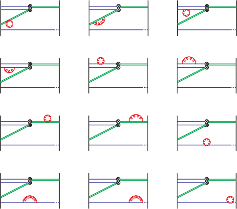
Figure 2: Feynman diagrams of the self-energy type.

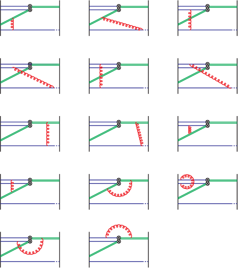
Figure 3: Feynman diagrams of the vertex type.

4.3 Matching to continuum schemes and consistency checks

The NLO anomalous dimension matrix of the operators (2) in continuum schemes can be found in [6], together with the one-loop matching relations to the minimal subtraction lattice scheme. The regularisations employed in [6] are DRED and NDR, and two possible subtraction prescriptions are considered, namely $\overline{\rm MS}$ and RI. An attractive feature of the latter is the independence of the corresponding anomalous dimension from the choice of evanescent operators (EO), which complicate the mixing pattern in $d=4-2\epsilon$ dimensions. As a consequence, it is trivial to perform a rotation of the anomalous dimension matrix in the RI scheme to a different basis of the physical operators, such as (46), without the need to address subtleties related to the definition of evanescent contributions. The choice of RI as a reference scheme is therefore convenient in order to make use of the two-loop matching relation (115) in the diagonal basis (46).

Results reported in [6] refer to a perturbative expansion in powers of the $\overline{\rm MS}$-coupling. We therefore need the matching coefficient in eq. (4.1), which relates $g_{\rm SF}$ to $g_{\overline{\rm MS}}$, to one-loop order. This has been calculated in [53] and is given by

$${\cal X}_{g}^{(1)} =2b_{0}\ln(\mu L)-\frac{1}{4\pi}\left(c_{1,0}+c_{1,1}N_{\rm f}\right)\ ,$$

$$c_{1,0} =1.25563(4)\ ,\quad c_{1,1}=0.039863(2)\ .$$ (123)

The NLO anomalous dimension of the operator basis (46) in the Feynman gauge ($\lambda=1$) and NDR regularisation, obtained from the covariant rotation $\gamma^{\prime(1)}=\Lambda\gamma^{(1)}\Lambda^{-1}$, is a diagonal matrix whose non-zero coefficients read

$$\gamma_{1;{\rm RI}}^{\prime+;(1)}=\frac{1}{(4\pi)^{4}}\bigg{[} -\frac{131+8\pi^{2}}{12}N^{2}+6N-\frac{1-2\pi^{2}}{3}+\frac{30+4\pi^{2}}{3N}-\frac{57+16\pi^{2}}{12N^{2}}$$

$$+N_{\rm\scriptsize f}\left(\frac{5}{3}N-\frac{5}{3N}\right)\bigg{]}\ ,$$

$$\gamma_{2;{\rm RI}}^{\prime+;(1)}=\frac{1}{(4\pi)^{4}}\bigg{[} -\frac{131+8\pi^{2}}{12}N^{2}+\frac{214}{9}N+\frac{301+6\pi^{2}}{9}+\frac{18-4\pi^{2}}{3N}+\frac{87-16\pi^{2}}{12N^{2}}$$

$$+N_{\rm\scriptsize f}\left(\frac{5}{3}N-\frac{40}{9}-\frac{55}{9N}\right)\bigg{]}\ ,$$

$$\gamma_{3;{\rm RI}}^{\prime+;(1)}=\frac{1}{(4\pi)^{4}}\bigg{[} -\frac{131+8\pi^{2}}{12}N^{2}-\frac{83}{6}N+\frac{309+8\pi^{2}}{12}-\frac{24-4\pi^{2}}{3N}+\frac{21-4\pi^{2}}{3N^{2}}$$

$$+N_{\rm\scriptsize f}\left(\frac{5}{3}N+\frac{10}{3}-\frac{5}{N}\right)\bigg{]}\ ,$$

$$\gamma_{4;{\rm RI}}^{\prime+;(1)}=\frac{1}{(4\pi)^{4}}\bigg{[} -\frac{131+8\pi^{2}}{12}N^{2}+\frac{71}{6}N+\frac{309+8\pi^{2}}{12}+\frac{42-4\pi^{2}}{3N}+\frac{33-4\pi^{2}}{3N^{2}}$$

$$+N_{\rm\scriptsize f}\left(\frac{5}{3}N-\frac{10}{3}-\frac{5}{N}\right)\bigg{]}\ .$$ (124)

The same rotation can be applied to the one-loop operator matching matrix ${\cal X}^{\prime(1)}_{{\rm RI,lat}}$. In this case the analytic dependence upon the gauge parameter $\lambda$ is needed in order to account for the derivative term included in the two-loop matching relation (115). With $N=3$, one has

$${\cal X}_{1;{\rm RI,lat(wilson)}}^{\prime(1)} =\frac{1}{(4\pi)^{2}}\left[\frac{10}{3}-\frac{8}{3}\lambda+(D_{LL}-D_{RR})\right]\ ,$$

$${\cal X}_{2;{\rm RI,lat(wilson)}}^{\prime(1)} =\frac{1}{(4\pi)^{2}}\left[\frac{10}{3}-\frac{8}{3}\lambda+D_{LL}^{S}\right]\ ,$$

$${\cal X}_{3;{\rm RI,lat(wilson)}}^{\prime(1)} =\frac{1}{(4\pi)^{2}}\left[\frac{10}{3}-\frac{8}{3}\lambda+\frac{1}{4}\left(2D_{LR}+2D^{S}_{LR}-4\bar{D}_{RL}-\bar{D}^{S}_{RL}\right)\right]\ ,$$

$${\cal X}_{4;{\rm RI,lat(wilson)}}^{\prime(1)} =\frac{1}{(4\pi)^{2}}\left[\frac{10}{3}-\frac{8}{3}\lambda+\frac{1}{4}\left(2D_{LR}+2D^{S}_{LR}+4\bar{D}_{RL}+\bar{D}^{S}_{RL}\right)\right]$$ (125)

for light quarks regularised with the pure Wilson action. If the $\mbox{O}(a)$ improved action is used instead, one has to add to them the matching factors between the two actions, viz.

$${\cal X}_{1;{\rm lat(sw),lat(wilson)}}^{\prime(1)} =\frac{1}{(4\pi)^{2}}\left[-\frac{4}{3}f^{I}-\frac{1}{3}v^{I}-\frac{4}{3}w^{I}\right]\ =0.038033(2)\ ,$$

$${\cal X}_{2;{\rm lat(sw),lat(wilson)}}^{\prime(1)} =\frac{1}{(4\pi)^{2}}\left[-\frac{4}{3}f^{I}-\frac{2}{9}v^{I}\right]\ =0.040240(2)\ ,$$

$${\cal X}_{3;{\rm lat(sw),lat(wilson)}}^{\prime(1)} =\frac{1}{(4\pi)^{2}}\left[-\frac{4}{3}f^{I}+\frac{2}{3}w^{I}\right]\ =0.034253(2)\ ,$$

$${\cal X}_{4;{\rm lat(sw),lat(wilson)}}^{\prime(1)} =\frac{1}{(4\pi)^{2}}\left[-\frac{4}{3}f^{I}+\frac{4}{3}w^{I}\right]\ =0.037720(2)\ ,$$ (126)

where the lattice integrals $f^{I}$, $v^{I}$ and $w^{I}$ are discussed in Appendix B. Numerical values of the $D$-coefficients, expressed in [6] as linear combinations of a basic set of lattice integrals, are reported in Table 3 of Appendix B, where a new computational method to improve their numerical accuracy is also described. The factors in eq. (126) are obtained from the coefficients denoted $D^{I}$ in [6], after subtracting the contributions coming from the $\mbox{O}(a)$ improvement of the four-fermion operators. All the ingredients needed to evaluate the RHS of eq. (115) have now been specified. The absence of operator mixing in the diagonal basis (46) implies that the commutator term in eq. (115) is identically zero. NLO anomalous dimensions in the previously introduced SF schemes follow from a straightforward use of eqs. (4.1), (116) and (122)–(4.3). We have collected the ratios of $\gamma_{k;\rm SF}^{\prime+;(1)}$ to the corresponding LO coefficients $\gamma_{k}^{\prime+;(0)}$ in Tables 10 – 15. In the matching we have employed the values of $r_{k,0}^{+}$ obtained with the pure Wilson action for light quarks, as they tend to display a better behaved continuum extrapolation, after the $\mbox{O}(a)$ contributions have been removed through blocking.

In order to check our results, we have also derived the SF NLO anomalous dimensions using $\overline{\rm MS}$ as a reference scheme. The matching procedure, rather delicate in this case, must take into account the rôle played by the EO in fixing the finite contributions to the NLO anomalous dimension matrix $\gamma^{{\scriptsize+};(1)}_{\overline{\rm MS}}$. A naive rotation of the latter is potentially hazardous without reconsidering the choice of the EO. An alternative approach is to work within the original basis (2), to which the results in [6] refer, and then rotate the one-loop matching coefficients from the SF to the lattice scheme according to the inverse rotation ${\cal X}_{\rm SF,lat}^{(1)}=\Lambda^{-1}{\cal X}_{\rm SF,lat}^{\prime(1)}\Lambda$. This is certainly possible, as the computation of such coefficients is performed on the lattice in $d=4$ dimensions, where no EO contributes. Of course, the commutator term in eq. (115) must be included in this case, whilst the gauge term proportional to $b_{0}^{\lambda}$ is not present. Once the NLO anomalous dimension matrix has been obtained in the SF scheme, a straight rotation back to the diagonal basis (46) yields the scalar coefficients $\gamma_{k;\rm SF}^{\prime+;(1)}$. This procedure has been applied using either DRED or NDR regularisations. In both cases we obtain the same results as with RI in the diagonal basis.

We have also verified that the difference between the finite parts of the SF renormalisation constants with improved and unimproved Wilson light quarks coincides with the values in eq. (126). The numerical values of these finite matching constants are indeed in perfect agreement with the analogous SF quantities.

We finally concentrate on the numerical values of the NLO anomalous dimension coefficients in the SF. A comparison with the case studied in [23], where the four-fermion operators contain only relativistic quark fields, shows that in the present case the variation of the anomalous dimension due to different choices of the SF boundary sources in the renormalisation condition is much less pronounced. Also, the non-perturbative identities in eq. (3) are verified explicitly by the one-loop results. The dependence on the value of the parameter $\alpha$ is very small, too. Finally, at $\theta=0.5$, which is commonly employed in non-perturbative studies of SF renormalisation, the values obtained for the ratios $\gamma_{k;\rm SF}^{\prime+;(1)}/\gamma_{k}^{\prime+;(0)}$ are relatively small, pointing towards a good convergence of the perturbative series, save for ${\cal{Q}}_{2}^{\scriptsize+}$, where they are close to $-0.5$. The question whether this is a relevant source of uncertainty in the NLO matching of renormalised matrix elements to continuum schemes is left for future studies.

4.4 One-loop order cutoff effects in step-scaling functions

The non-perturbative RG-evolution of the four-quark operators in the diagonal basis (46) is obtained through the computation of the step-scaling functions

$$\sigma_{k;\alpha}^{{\scriptsize+};(s)}(u)=\lim_{a\to 0}\Sigma_{k;\alpha}^{{\scriptsize+};(s)}(u,a/L)\ ,\qquad\Sigma_{k;\alpha}^{{\scriptsize+};(s)}(u,a/L))=\frac{{\cal Z}_{k;\alpha}^{\prime+;(s)}(g_{0},a/2L)}{{\cal Z}_{k;\alpha}^{\prime+;(s)}(g_{0},a/L)}\biggr{|}_{\bar{g}^{2}(L)=u}\ .$$ (127)

These ratios of renormalisation constants provide the operator running between the scales $\mu=1/L$ and $\mu=1/2L$. The advantage of introducing such ratios is related to the compensation of logarithmic divergences between numerator and denominator, thus resulting in a finite continuum limit. Cutoff effects can be therefore completely decoupled from the continuum RG-evolution. We are concerned here with the perturbative expansion of (127) in the renormalised coupling, that is

$$\sigma_{k;\alpha}^{{\scriptsize+};(s)}(u)=1+\sigma_{k;\alpha}^{{\scriptsize+};(s,1)}u+\sigma_{k;\alpha}^{{\scriptsize+};(s,2)}u^{2}+{\rm O}(u^{3})\,.$$ (128)

The first two terms of this expansion depend upon the LO and NLO anomalous dimension coefficients. They read explicitely

$$\sigma_{k;\alpha}^{{\scriptsize+};(s,1)} =\gamma_{k}^{\prime{\scriptsize+};(0)}\ln 2\ ,$$

$$\sigma_{k;\alpha}^{{\scriptsize+};(s,2)} =\gamma_{k;\rm SF}^{\prime{\scriptsize+};(1)}\ln 2+\left[\frac{1}{2}(\gamma_{k}^{\prime{\scriptsize+};(0)})^{2}+b_{0}\gamma_{k}^{\prime{\scriptsize+};(0)}\right](\ln 2)^{2}\,.$$ (129)

A graphical representation of (128) for the whole operator basis in some particular cases is provided by the four plots of Figures 4 and 5, in the range of values of $g^{2}_{\rm SF}$ used in previous non-perturbative studies by the ALPHA Collaboration.

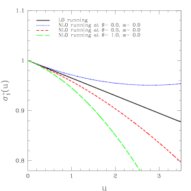
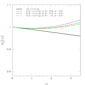
Figure 4: On the left(right) side the step scaling function of ${\cal Q}_{1}^{\prime+}$(${\cal Q}_{2}^{\prime+}$) at NLO and $N_{\rm f}=0$ is plotted vs. the squared renormalised coupling in the SF scheme. The boundary sources choice is $s=1$, and the $\alpha$-parameter is set to zero.

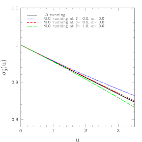
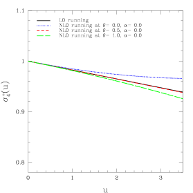
Figure 5: On the left(right) side the step scaling function of ${\cal Q}_{3}^{\prime+}$(${\cal Q}_{4}^{\prime+}$) at NLO and $N_{\rm f}=0$ is plotted vs. the renormalised coupling in the SF scheme. The boundary sources choice is $s=1$, and the $\alpha$-parameter is set to zero.

The rate of convergence of the step-scaling functions toward the continuum limit at LO can be expressed in terms of the first non-trivial coefficient of the perturbative expansion (analogous to (128)) of $\Sigma_{k;\alpha}^{{\scriptsize+};(s)}(u,a/L)$ via the ratio

$$\delta_{k;\alpha}^{{\scriptsize+};(s)}(a/L)=\frac{\Sigma_{k;\alpha}^{{\scriptsize+};(s,1)}(a/L)-\sigma_{k;\alpha}^{{\scriptsize+};(s,1)}}{\sigma_{k;\alpha}^{{\scriptsize+};(s,1)}}\ ,$$ (130)

where

$$\Sigma_{k;\alpha}^{{\scriptsize+};(s,1)}(a/L)={\cal Z}_{k;\alpha}^{\prime+;(s,1)}(2L/a)-{\cal Z}_{k;\alpha}^{\prime+;(s,1)}(L/a)\ .$$ (131)

In order to compare the perturbative lattice artefacts (130) with the ones obtained from the corresponding non-perturbative Monte Carlo simulations, the same definition of the critical mass, based on the PCAC Ward identity, should be adopted. This point has been extensively explained in [23], where the numerical values of $am_{c}^{(1)}(L/a)$ from $L/a=6$ to $L/a=32$ have been provided (cf. Table 3 in that work). That discussion will not be repeated here. Since our codes ran up to $L/a=48$, we are in the position to extend the aforementioned table to include the additional points. The new numbers are reported in Table 1.

$L/a$	$am_{c}^{(1)}(L/a)|_{c_{\rm sw}=1}/C_{\rm F}$	$am_{c}^{(1)}(L/a)|_{c_{\rm sw}=0}/C_{\rm F}$
34	-0.20255637783	-0.32544080501
36	-0.20255639414	-0.32547023220
38	-0.20255640819	-0.32549515390
40	-0.20255642028	-0.32551644442
42	-0.20255643068	-0.32553477599
44	-0.20255643965	-0.32555067224
46	-0.20255644740	-0.32556454600
48	-0.20255645412	-0.32557672619

Table 1: The one-loop coefficients of the critical mass as obtained from the PCAC Ward Identity at finite lattice size. For the parameter choices made here, the convergence to the values at infinite lattice size is quadratic/cubic in $(a/L)$, for standard/${\rm O}(a)$ improved Wilson quarks.

In practice, non-perturbative simulations based on the Eichten-Hill discretisation of the heavy quark fields should better be avoided, given the bad intrinsic signal-to-noise ratio (3, 4) [27]. Nevertheless, it is instructive to compute lattice artefacts in perturbation theory for the Eichten-Hill action, if only to check whether the use of static fields enhances lattice artefacts with respect to the purely relativistic case. A comparison between static-light and light-light four-quark operators in a typical situation is shown in Figure 6. All data refer to ${\cal Q}_{1}^{\scriptsize+}$, employing a renormalisation scheme in which the boundary sources have a Dirac structure $[\gamma_{5},\gamma_{5},\gamma_{5}]$ and where the normalisation of the four-quark correlator involves only $f_{1}^{ll}$. Relativistic data are taken from [23]. Taken at face value, the plot leads to the conclusion that the light quark action is the main responsible for the presence of relatively large lattice artefacts: once this has been chosen, static-light and light-light four-quark operators come to be affected by cutoff effects of a similar size.

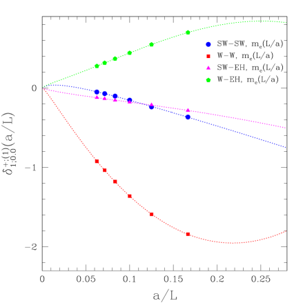
Figure 6: Comparison between cutoff effects of the step scaling function of the static-light and light-light versions of the four-quark operator ${\cal Q}_{1}^{\prime{\scriptsize+}}$. Light quarks are described in terms of the unimproved (W) or improved (SW) Wilson action. Static quarks are always described by the Eichten-Hill (EH) action. The critical mass has been obtained from the PCAC Ward Identity.

5 tmQCD for $B^{0}$–$\bar{B}^{0}$ mixing

As stated above, our interest in the renormalisation of ${\cal Q}^{+}_{k}$ stems from the fact that the physical $\Delta B=2$ matrix elements involving the operators $Q^{+}_{1},Q^{+}_{2}$, with $\psi_{1}=\psi_{2}\equiv\psi_{\ell}$ (where in practice the flavour label $\ell$ denotes either a $d$ or an $s$ quark), can be mapped onto matrix elements of ${\cal Q}^{+}_{1},{\cal Q}^{+}_{2}$ computed in some suitable tmQCD regularisation. This reduces to a minimum the uncertainties related to operator renormalisation, which takes place essentially in the same way as if exact chiral symmetry were present. Now we will construct specific tmQCD regularisations which realize this mapping. This technique is a generalisation of the ones already developed for $B_{K}$ [20, 22].

We will work in the so-called “twisted basis”, and concentrate first on the case of the $B_{B}$ parameter where $\psi_{\ell}=d$. Let us consider a quark doublet $\psi^{T}=(u,d)$, for which we specify the tmQCD action

$$S^{\rm tmQCD}[\psi,\bar{\psi}]=a^{4}\sum_{x}\ \left\{\bar{\psi}(x)\left[D_{\rm w}+m+i\mu\tau^{3}\gamma_{5}\right]\psi(x)\right\}\,,$$ (132)

where $D_{\rm w}$ is the usual Wilson-Dirac operator (with or without a SW term). The choice of action for the other relativistic quark flavours is immaterial to the argument. The equivalence of tmQCD to standard QCD has been first established in [20]. Given a multi-local gauge-invariant operator ${\cal O}(x_{1},\dots,x_{n})$, the equivalence amounts to the identity between renormalised correlation functions

$$\langle\tilde{\cal O}_{\rm R}(x_{1},\dots,x_{n})\rangle_{(M_{\rm R},0)}=\langle{\cal O}_{\rm R}(x_{1},\dots,x_{n})\rangle_{(m_{\rm R},\mu_{\rm R})}\ ,$$ (133)

which holds in the regularised theory up to cutoff effects, and is exact in the continuum limit. In the above expression, the relation between the operators $\tilde{\cal O}$ and ${\cal O}$ is provided by the axial rotation of the quark fields which relates QCD to tmQCD, viz.

$$\begin{split}\tilde{\psi}&=\exp\left(i\alpha\gamma_{5}\tau^{3}/2\right)\psi\\ \tilde{\bar{\psi}}&=\bar{\psi}\exp\left(i\alpha\gamma_{5}\tau^{3}/2\right)\ ,\end{split}$$ (134)

where the twist angle $\alpha$ is defined in terms of the renormalised mass parameters of the tmQCD action as

$$\tan(\alpha)=\frac{\mu_{\rm R}}{m_{\rm R}}\,,$$ (135)

and the physical renormalised quark mass $M_{\rm R}$ is given by

$$M_{\rm R}=\sqrt{m_{\rm R}^{2}+\mu_{\rm R}^{2}}\,.$$ (136)

Let us now consider the static-light four-quark operators ${\cal O}^{\scriptsize+}_{\rm VV+AA}$ and ${\cal O}^{\scriptsize+}_{\rm VA+AV}$ with light flavours $\psi_{1}=\psi_{2}=d$. We observe that the rotation (134) implies

$$\tilde{\cal O}^{\scriptsize+}_{\rm VV+AA}=\cos(\alpha){\cal O}^{\scriptsize+}_{\rm VV+AA}-i\sin(\alpha){\cal O}^{\scriptsize+}_{\rm VA+AV}\ .$$ (137)

In particular, at $\alpha=\pi/2$, which is known as the maximally twisted case, (137) simplifies to

$$\tilde{\cal O}^{\scriptsize+}_{\rm VV+AA}=-i{\cal O}^{\scriptsize+}_{\rm VA+AV}\ .$$ (138)

Exactly the same property holds for the operator ${\rm SS+PP}$, for which one finds again

$$\tilde{\cal O}^{\scriptsize+}_{\rm SS+PP}=-i{\cal O}^{\scriptsize+}_{\rm SP+PS}\ .$$ (139)

This demonstrates explicitly that the matrix elements of ${\cal O}^{\scriptsize+}_{\rm VV+AA}$ and ${\cal O}^{\scriptsize+}_{\rm SS+PP}$, responsible for the particle mixing in the SM and within the static approximation of QCD, can be obtained from a computation of the matrix element of ${\cal O}^{\scriptsize+}_{\rm VA+AV}$ and ${\cal O}^{\scriptsize+}_{\rm SP+PS}$ in tmQCD at $\alpha=\pi/2$. Since in mass independent schemes, such as the SF, all dependence of renormalisation factors on the mass parameters drops out, it is clear that tmQCD does not spoil the renormalisation pattern of the operator basis (46). In particular, the combinations ${\cal Q}_{1}^{\prime}\equiv{\cal O}^{\scriptsize+}_{\rm VA+AV}$ and ${\cal Q}_{2}^{\prime}\equiv{\cal O}^{\scriptsize+}_{\rm VA+AV}+4{\cal O}^{\scriptsize+}_{\rm SP+PS}$ renormalise purely multiplicatively.

In case one is interested in the $B_{s}^{0}$–$\bar{B}_{s}^{0}$ mixing amplitude, it is enough to maximally twist a quark doublet which contains the $s$ quark, e.g. $(c,s)$, the action for which would read exactly as eq. (132), save for the eventual introduction of non-degenerate masses for the two quarks of the doublet, along the lines of [54]. The action for a twisted $(c,s)$ doublet would then read

$$S^{\rm tmQCD}[\psi,\bar{\psi}]=a^{4}\sum_{x}\ \left\{\bar{\psi}(x)\left[D_{\rm w}+\mathbf{m}+i\boldsymbol{\mu}\gamma_{5}\right]\psi(x)\right\}$$ (140)

with $\mathbf{m}={\rm diag}(m_{c},m_{s})$ and $\boldsymbol{\mu}={\rm diag}(\mu_{c},\mu_{s})$, and the constraint

$$\tan(\alpha)=-\frac{\mu_{s,{\rm R}}}{m_{s,{\rm R}}}=\frac{\mu_{c,{\rm R}}}{m_{c,{\rm R}}}\,.$$ (141)

A potential shortcoming of eq. (140) comes about in case it is taken as the action for dynamical $c,s$ quarks, since $M_{s,{\rm R}}\neq M_{c,{\rm R}}$ would then induce a phase in the fermion determinant. One may then consider more sophisticated chiral rotations that keep the determinant real, as in [55]. If $c,s$ are kept quenched, or interpreted as valence quarks, no such subtlety arises.

We conclude that the use of suitable tmQCD regularisations avoids the need of determining mixing coefficients for the renormalisation of the matrix elements entering the $B^{0}$–$\bar{B}^{0}$ amplitude in the static approximation. For an alternative analysis of operator mixing using a different tmQCD regularisation, we refer the reader to ref. [56].

An additional advantage brought in by the use of maximally tmQCD is the automatic $\mbox{O}(a)$ improvement of bare matrix elements of the above four-fermion operators. This property does not hold, on the other hand, for the renormalisation constants computed within the SF schemes discussed in previous sections. In order to obtain O($a$) improved renormalization constants one should use modified SF schemes, as proposed in refs. [57, 58].

In order to show that the bare matrix elements are automatically O($a$) improved we extend the argument in Appendix A of ref. [59]. The first observation is that, at maximal twist, the only O($a$) counterterms to the static action are proportional to the dimension five operators

$$\mbox{tr}(\boldsymbol{\mu}^{2})\,(\bar{\psi}_{h}\psi_{h}+\bar{\psi}_{\bar{h}}\psi_{\bar{h}})\,,~{}~{}~{}~{}~{}~{}~{}~{}~{}~{}(\mbox{tr}(\boldsymbol{\mu}))^{2}\,(\bar{\psi}_{h}\psi_{h}+\bar{\psi}_{\bar{h}}\psi_{\bar{h}})\,.$$ (142)

(In the simple case $\boldsymbol{\mu}=\mu\tau^{3}$ there is one single counterterm proportional to $\mu^{2}(\bar{\psi}_{h}\psi_{h}+\bar{\psi}_{\bar{h}}\psi_{\bar{h}})$.) These counterterms merely generate a shift of the static quark self-energy . The second observation is that all the possible O($a$) (dimension seven) counterterms will have the same static field content of the original (dimension six) four-fermion operator, and will differ from it only by the addition of mass factors or derivatives. It is then possible to extend the symmetry ${\cal P}\times{\cal D}_{d}\times(\mu\to-\mu)$ of the relativistic action [59] (where $\cal P$ is the physical parity and ${\cal D}_{d}$ is defined in ref. [60]) to include static quarks. ${\cal P}$ and ${\cal D}_{d}$ will now be defined to be

$${\cal{P}}:\left\{\begin{array}[]{lll}U_{0}(x)&\rightarrow&U_{0}(x^{\pi})\\ U_{k}(x)&\rightarrow&U_{k}^{\dagger}(x^{\pi}-a\hat{k})\\ \psi(x)&\rightarrow&i\gamma_{0}\gamma_{5}\tau_{3}\psi(x^{\pi})\\ \bar{\psi}(x)&\rightarrow&\bar{\psi}(x^{\pi})\tau_{3}\gamma_{5}\gamma_{0}i\\ \psi_{h}(x)&\rightarrow&\psi_{h}(x^{\pi})\\ \bar{\psi}_{h}(x)&\rightarrow&\bar{\psi}_{h}(x^{\pi})\\ \psi_{\bar{h}}(x)&\rightarrow&-\psi_{\bar{h}}(x^{\pi})\\ \bar{\psi}_{\bar{h}}(x)&\rightarrow&-\bar{\psi}_{\bar{h}}(x^{\pi})\end{array}\right. {\cal{D}}_{d}:\left\{\begin{array}[]{lll}U_{\mu}(x)&\rightarrow&U_{\mu}^{\dagger}(-x-a\hat{\mu})\\ \psi(x)&\rightarrow&-i\psi(-x)\\ \bar{\psi}(x)&\rightarrow&-i\bar{\psi}(-x)\\ \psi_{h}(x)&\rightarrow&\psi_{\bar{h}}(-x)\\ \bar{\psi}_{h}(x)&\rightarrow&\bar{\psi}_{\bar{h}}(-x)\\ \psi_{\bar{h}}(x)&\rightarrow&\psi_{h}(-x)\\ \bar{\psi}_{\bar{h}}(x)&\rightarrow&\bar{\psi}_{h}(-x)\end{array}\right.$$ (158)

where $(x_{0},{\mathbf{x}})^{\pi}=(x_{0},-{\mathbf{x}})$. Using ${\cal P}\times{\cal D}_{d}\times(\mu\to-\mu)$ one immediately concludes that all the relevant dimension seven operators have opposite parity with respect to the dimension six ones. Using the same arguments of ref. [59], one then concludes that no O($a$) appears in the Symanzik expansion of the relevant correlation functions.

6 Conclusions

In this paper we have shown that the renormalisation problem of heavy-light four-quark operators in the static approximation can be tackled for Wilson-like fermions without the need to perform finite subtractions.

Owing to the presence of static quark fields, the flavour switching symmetries, which in the relativistic case have proved so useful [61, 19] for imposing constraints on the mixing, are very much reduced. However, this lack is compensated by the heavy quark symmetry, spatial rotations and a set of discrete symmetries, such as time reversal. The emerging renormalisation and mixing pattern is then quite similar to the relativistic theory: while chiral symmetry breaking generated by the Wilson term induces mixing among different chiralities of parity-even operators in the lattice regularised theory, such mixings are completely absent in the parity-odd sector.

Twisted-mass QCD can be used to relate the operator bases in the parity-even and parity-odd sectors also in the static approximation. In particular, we have shown how to do this for the operators that contribute to $B^{0}$–$\bar{B}^{0}$ mixing in the Standard Model, using a maximal twist setup that brings in, as a bonus, the potential for automatic $\mbox{O}(a)$ improvement.

A fully non-perturbative determination of the renormalisation factors of four-quark operators in the framework of the Schrödinger functional appears entirely feasible at this point, provided that one can overcome the well-known problem of the Eichten-Hill action, namely the exponential growth of statistical fluctuations at large Euclidean times [68]. Here the hope is that the methods described in refs. [62, 27] turn out to be as useful as in the simpler case of heavy-light bilinears.

We have verified explicitly the expected mixing pattern in an extensive perturbative calculation at one loop. Thereby we have also obtained the NLO anomalous dimensions, which will be an important ingredient in future non-perturbative determinations of the renormalisation factors. Furthermore, our perturbative calculation can be used to optimise the choice of renormalisation prescription in the forthcoming numerical simulations.

As we have mentioned above, at the level of $B^{0}$–$\bar{B}^{0}$ amplitudes the matching between HQET and QCD requires to compute matrix elements of the operators ${\cal O}^{+}_{\rm VV+AA}$ and ${\cal O}^{+}_{\rm SS+PP}$, which are mapped via tmQCD onto the operators ${\cal O}^{+}_{\rm VA+AV}$ and ${\cal O}^{+}_{\rm SP+PS}$. Therefore, as far as renormalisation is concerned, one is then faced with the task of computing the step-scaling functions for the relevant pair of operators, which renormalise multiplicatively, i.e. ${\cal O}^{+}_{\rm VA+AV}$ and ${\cal O}^{+}_{\rm VA+AV}+4{\cal O}^{+}_{\rm SP+PS}$.

The static approximation considered in this work only represents the lowest order of HQET, and hence all results for phenomenologically relevant quantities are subject to corrections in powers of the inverse heavy quark mass. While there are strategies in place which are designed for determining the leading $1/M$ corrections non-perturbatively [14], it is also possible to interpolate lattice results between the static approximation and the regime of relativistic quarks with masses around that of the charm quark. Our findings may serve to obtain high-precision results for $B^{0}-\bar{B}^{0}$ mixing amplitudes in the static approximation, which in turn are required to perform reliable interpolations to the physical $b$-quark mass.

Acknowledgements

We are grateful to J. Heitger and R. Sommer for their participation in the early stages of this work. We thank D. Bećirević, M. Della Morte, F. Mescia and especially J. Reyes for useful discussions. F.P. acknowledges the Alexander-von-Humboldt Stiftung for financial support. Hospitality offered by CERN (F.P., M.P.) and DESY (C.P.) during the preparation of this work is thankfully acknowledged.

Appendix A Constraints from heavy quark spin symmetry and $H(3)$ spatial rotations on the mixing pattern

We now describe the procedure followed to impose the constraints from heavy quark spin symmetry and cubic rotations. It applies identically to both the parity-even and the parity-odd sectors and we choose to describe it for the latter. It turns out that, in this particular case, there is no need for considering a maximal set of independent symmetry transformations, because the final constraints are already obtained by considering a finite spin transformation of the heavy fields, e.g.

$$\Phi_{1}:\qquad \bar{\psi}_{h}\to\bar{\psi}_{h}\gamma_{2}\gamma_{3}\ ,\quad\bar{\psi}_{\bar{h}}\to\bar{\psi}_{\bar{h}}\gamma_{2}\gamma_{3}\ ,$$ (159)

and two lattice spatial rotations, e.g.

$$\Phi_{2}:\qquad{\cal R}(\ \hat{1}\to\hat{2}\ )\ \mbox{rotates the $\hat{1}$ axis onto the $\hat{2}$ axis},$$

$$\Phi_{3}:\qquad{\cal R}(\ \hat{2}\to\hat{3}\ )\ \mbox{rotates the $\hat{2}$ axis onto the $\hat{3}$ axis,}$$ (160)

alone. The subspace spanned by (2) is not invariant under the set of transformations (159). We hence give up temporarily Lorentz invariance (which, as we will see, will be recovered naturally) and consider an enlarged basis containing eight operators,

$${\cal O}^{\pm}=({\cal O}^{\pm}_{V_{0}A_{0}+A_{0}V_{0}},\dots,{\cal O}^{\pm}_{V_{3}A_{3}+A_{3}V_{3}},{\cal O}^{\pm}_{V_{0}A_{0}-A_{0}V_{0}},\dots,{\cal O}^{\pm}_{V_{3}A_{3}-A_{3}V_{3}})^{T}\ ,$$ (161)

which can generate, when properly combined, the original parity-odd basis (2) . The analysis performed in section 2 by using chiral symmetry can be carried over to (161), which can be accordingly shown to renormalise as

$${\cal O}^{\pm}_{R}=z^{\pm}(\mathds{1}+\delta^{\pm}){\cal O}^{\pm}\ .$$ (162)

Here $z^{\pm}$ are block diagonal matrices containing two $(4\times 4)$ scale-dependent blocks while $\delta^{\pm}$ are block off-diagonal matrices, containing two $(4\times 4)$ scale-independent blocks. The advantage of using (161) is that the new basis is closed under (159) and (A), and the matrices $\Phi_{k}$ that implement the symmetry rotations can be constructed explicitly. Moreover, it should be observed that in order to preserve the renormalisation structure determined by chiral symmetry, the two matrices $z^{\pm}$ and $\delta^{\pm}$ have to satisfy the symmetry constraints independently, namely

$$z^{\pm} =\Phi_{k}z^{\pm}\Phi_{k}^{-1}\ ,$$

$$\delta^{\pm} =\Phi_{k}\delta^{\pm}\Phi_{k}^{-1}\ .$$ (163)

The explicit form of the matrices $\Phi_{k}$ is easily found out to be:

$$\Phi_{1}=\left(\begin{array}[]{rrrrrrrr}0&1&0&0&0&0&0&0\\ 1&0&0&0&0&0&0&0\\ 0&0&0&1&0&0&0&0\\ 0&0&1&0&0&0&0&0\\ 0&0&0&0&0&-1&0&0\\ 0&0&0&0&-1&0&0&0\\ 0&0&0&0&0&0&0&1\\ 0&0&0&0&0&0&1&0\\ \end{array}\right)\ ,\quad\Phi_{2}=\left(\begin{array}[]{rrrrrrrr}1&0&0&0&0&0&0&0\\ 0&0&1&0&0&0&0&0\\ 0&1&0&0&0&0&0&0\\ 0&0&0&1&0&0&0&0\\ 0&0&0&0&1&0&0&0\\ 0&0&0&0&0&0&1&0\\ 0&0&0&0&0&1&0&0\\ 0&0&0&0&0&0&0&1\\ \end{array}\right)\ ,\quad\Phi_{3}=\left(\begin{array}[]{rrrrrrrr}1&0&0&0&0&0&0&0\\ 0&1&0&0&0&0&0&0\\ 0&0&0&1&0&0&0&0\\ 0&0&1&0&0&0&0&0\\ 0&0&0&0&1&0&0&0\\ 0&0&0&0&0&1&0&0\\ 0&0&0&0&0&0&0&1\\ 0&0&0&0&0&0&1&0\\ \end{array}\right)\ .$$ (188)

Once all the constraints are imposed one gets :

$$z^{\pm}=\left(\begin{array}[]{rrrrrrrr}z_{1}&z_{2}&z_{2}&z_{2}&0&0&0&0\\ z_{2}&z_{1}&z_{2}&z_{2}&0&0&0&0\\ z_{2}&z_{2}&z_{1}&z_{2}&0&0&0&0\\ z_{2}&z_{2}&z_{2}&z_{1}&0&0&0&0\\ 0&0&0&0&z^{\prime}_{1}&-z^{\prime}_{2}&-z^{\prime}_{2}&-z^{\prime}_{2}\\ 0&0&0&0&-z^{\prime}_{2}&z^{\prime}_{1}&z^{\prime}_{2}&z^{\prime}_{2}\\ 0&0&0&0&-z^{\prime}_{2}&z^{\prime}_{2}&z^{\prime}_{1}&z^{\prime}_{2}\\ 0&0&0&0&-z^{\prime}_{2}&z^{\prime}_{2}&z^{\prime}_{2}&z^{\prime}_{1}\\ \end{array}\right)\ ,\quad\delta^{\pm}=\left(\begin{array}[]{rrrrrrrr}0&0&0&0&-\delta_{1}&\delta_{2}&\delta_{2}&\delta_{2}\\ 0&0&0&0&-\delta_{2}&\delta_{1}&\delta_{2}&\delta_{2}\\ 0&0&0&0&-\delta_{2}&\delta_{2}&\delta_{1}&\delta_{2}\\ 0&0&0&0&-\delta_{2}&\delta_{2}&\delta_{2}&\delta_{1}\\ -\delta^{\prime}_{1}&-\delta^{\prime}_{2}&-\delta^{\prime}_{2}&-\delta^{\prime}_{2}&0&0&0&0\\ \delta^{\prime}_{2}&\delta^{\prime}_{1}&\delta^{\prime}_{2}&\delta^{\prime}_{2}&0&0&0&0\\ \delta^{\prime}_{2}&\delta^{\prime}_{2}&\delta^{\prime}_{1}&\delta^{\prime}_{2}&0&0&0&0\\ \delta^{\prime}_{2}&\delta^{\prime}_{2}&\delta^{\prime}_{2}&\delta^{\prime}_{1}&0&0&0&0\\ \end{array}\right)\ .$$ (205)

Now we go to a basis such that $z^{\pm}$ is diagonal. A convenient choice is:

$$\{{\cal Q}^{\pm}_{1},{\cal Q}^{\pm}_{1}+4{\cal Q}^{\pm}_{2},R_{1}^{\pm},R_{2}^{\pm},{\cal Q}^{\pm}_{3}+2{\cal Q}^{\pm}_{4},{\cal Q}^{\pm}_{3}-2{\cal Q}^{\pm}_{4},R_{3}^{\pm},R_{4}^{\pm}\}\ ,$$ (206)

where $R_{j}^{\pm}$ are some Lorentz non-invariant operators, the precise expression of which is irrelevant for the rest of the argument. By transforming into this basis it turns out that also the nontrivial blocks of $\delta^{\pm}$ are diagonal. We have therefore arrived to the final conclusion that the basis (46) is closed under renormalisation, with the mixing pattern presented in (63).

Appendix B Integrals in the infinite volume theory

The lattice contributions to the matching coefficients ${\cal X}^{(1)}_{{\rm ref,lat}}$, commonly expressed in terms of a basic set of Feynman integrals in the momentum-space representation, have been calculated and cross-checked by independent authors [63, 6, 64, 65]. In all cases, their evaluation has been pursued through Monte Carlo simulations (VEGAS), resulting in an average numerical precision of three digits. On the other hand, the matching constants ${\cal X}_{\rm SF,lat}^{(1)}$, which provide the connection between the SF and the lattice scheme, have been calculated with a better accuracy, as explained in section 4.2. As a consequence, the uncertainty on the NLO coefficients of the SF anomalous dimensions is dominated by the lack of precision in the infinite lattice integrals. A possible way out would be running the Monte Carlo algorithms on faster computers and wait long enough for a couple of digits more. A more attractive alternative is to use an analytical trick to improve the quality of the results, obtaining at the same time some insight into the peculiar nature of the static lattice integrals. As an example, we consider

$$d_{1} =\frac{1}{\pi^{2}}\int_{-\pi}^{\pi}d^{4}k\biggl{[}-4\theta(1-k^{2})\frac{1}{k^{4}}+\frac{1}{4\Delta_{1}\Delta_{2}}+\frac{3}{16}\frac{1}{\Delta_{2}}\biggr{]},$$

$$\Delta_{1} =\sum_{\mu=1}^{4}\sin^{2}\frac{k_{\mu}}{2}\ ,\qquad\Delta_{2}=\sum_{\mu=1}^{4}\sin^{2}k_{\mu}+4\Delta_{1}^{2}\ .$$ (207)

The first term in the integral, which comes from the static propagator, diverges logarithmically at $k=0$. This contribution is compensated by an opposite divergence of the subsequent terms, which brings the final result to a finite value, namely $d_{1}\simeq 5.46$. In principle, $d_{1}$ could be regularised through the usual lattice discretisation of the integration variables,

$$k_{\mu}\ \rightarrow\ \frac{2\pi}{N}n_{\mu}\ ,\qquad-\frac{N}{2}<n_{\mu}\leq\frac{N}{2}\ .$$ (208)

If it were not for the $\theta(1-k^{2})$-function, the integral would be expected to behave like an ordinary lattice integral, i.e. its convergence to the continuum would be determined by the asymptotic formula

$$\tilde{d}_{1}(N)=d_{1}+\frac{a_{1}}{N}+\frac{b_{1}}{N}\log(N)+\frac{a_{2}}{N^{2}}+\frac{b_{2}}{N^{2}}\log(N)+O\left(\frac{1}{N^{3}}\right)\ ,$$ (209)

where $\tilde{d}_{1}$ represents the lattice version of $d_{1}$. The $\theta$-function, which is non-zero inside a spherical domain, produces an explicit breaking of the hyper-cubic $H(4)$ symmetry, thus perturbing the convergence pattern. This effect can be better understood by defining

$$I\equiv\int_{-\pi}^{\pi}d^{4}k\ \theta(1-k^{2})\frac{1}{k^{4}}\quad\longrightarrow\quad\tilde{I}(N)=\frac{1}{\pi^{2}}\sum_{n_{i}:\ n^{2}\neq 0}\frac{\theta\left(\frac{N^{2}}{4\pi^{2}}-n^{2}\right)}{n^{4}}\ ,$$ (210)

and observing that the number of the lattice points that lie inside a 3-sphere $\Sigma$ with radius $R_{\Sigma}=N/2\pi$ increases irregularly when $N\to\infty$. The alternating excess or deficit of integration points gives rise to the oscillating behaviour characterising the dashed curve of Figure 4. In order to smooth $\tilde{d}_{1}$, we propose to regularise $\tilde{I}$ in a way that formally restores the hyper-cubic symmetry. To this aim, we introduce an order parameter $\Delta V_{\Sigma}$, which provides a measure of the spherical symmetry breaking produced by the lattice discretisation,

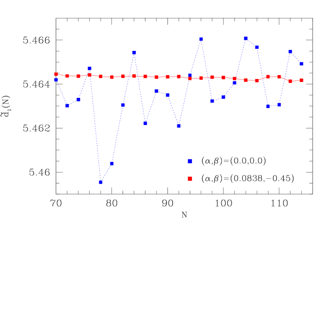
Figure 7: Convergence pattern of $\tilde{d}_{1}(N)$.

$$\Delta V_{\Sigma}(N)=\frac{V_{\Sigma}-\tilde{V}_{\Sigma}(N)}{V_{\Sigma}}\ .$$ (211)

Here $V_{\Sigma}=N^{4}/(32\pi^{2})$ is the volume of the above-mentioned 3-sphere, and $\tilde{V}_{\Sigma}(N)$ represents the corresponding lattice volume, obtained by just counting the number of the lattice points that belong to the inner of $\Sigma$ at fixed $N$. The recovery of spherical symmetry in the continuum limit implies that $\Delta V_{\Sigma}$ vanishes when $N\to\infty$. In addition, $\Delta V_{\Sigma}$ describes a surface effect at large values of $N$, and its rate of vanishing is therefore proportional to $1/N$, up to fluctuations. We now define

$$\tilde{I}^{\prime}(N)=\left\{1+\alpha\Delta V_{\Sigma}(N)+\beta\Delta V_{\Sigma}(N)^{2}\right\}\tilde{I}(N)\ ,$$ (212)

where $\alpha$ and $\beta$ are two real parameters to be suitably chosen. Although both $\tilde{I}$ and $\tilde{I}^{\prime}$ diverge in the continuum limit, their difference vanishes. According to our considerations, the fluctuations of $\Delta V_{\Sigma}$ are expected to mimic the ones of $\tilde{I}$, and an appropriate and unique choice of $\alpha$ and $\beta$ will provide a partial cancellation of the irregularities observed in the continuum approach of $\tilde{I}^{\prime}$, and consequently $\tilde{d}_{1}$. The search of optimal values can be simply performed by hand, as far as only two parameters have to be tuned (in addition, $\beta$ multiplies a subdominant contribution). We find, in particular, $(\alpha,\beta)=(0.0838,-0.45)$. A plot of $\tilde{d}_{1}$, regularised according to this choice, is represented by the solid curve in Figure 4. A fit of the smoothed data against (209) allows to extract the value of $d_{1}$ with much higher precision than the previous determinations. The procedure can be extended to all the other lattice integrals which contribute to the matching between the continuum and the lattice heavy-light operators. Their explicit expressions, reported in [29, 6], will not be reproduced here, but a list of more accurate values, obtained with the method explained above, is given in Table 2.

$d_{1}$	$J_{1}$	$f$	$v$	$c$	$w$
$5.4636(6)$	$-4.8540(6)$	$13.3503(6)$	$-6.9230(24)$	$4.5259(27)$	$-1.20538(1)$

Table 2: Some basic infinite lattice integrals, which are needed to compute the matching coefficients ${\cal X}^{(1)}_{{\rm ref,lat}}$. Their values have been determined according to the regularisation method explained in this Appendix.

The finite lattice constants that contribute to the matching coefficients ${\cal X}^{(1)}_{{\rm ref,lat}}$ are expressed in terms of those lattice integrals by a set of algebraic relations that have been first published in [29, 6]. Their values are reported in Table 3.

$\ D_{LL}\$	$-41.248(8)$	$\ \bar{D}_{LL}\$	$2.5923(12)$
$\ D^{S}_{LL}\$	$-30.879(8)$	$\ \bar{D}_{RL}\$	$2.4489(11)$
$\ D_{LR}\$	$-37.843(6)$	$\ \bar{D}_{RR}\$	$0.40179(3)\$
$\ D^{S}_{LR}\$	$-37.843(6)$	$\ \bar{D}^{S}_{RL}\$	$9.796(4)$
$\ D_{RR}\$	$-1.60717(1)$

Table 3: Values of the combinations of lattice integrals entering matching coefficients.

The improvement integrals $f^{I}$, $v^{I}$ and $w^{I}$, introduced in eq. (126), do not involve a factor of $\theta(1-k^{2})$. Hence, their numerical value can be computed with good precision through the blocking procedure described in [52]. We obtain:

$$f^{I} =-3.6461(2)\ ,$$

$$v^{I} =-6.7185(2)\ ,$$

$$w^{I} =0.82130(2)\ .$$ (213)

Appendix C Tables.

In this appendix we list our results for the coefficients $r^{+}_{k,0}$, as well as for the NLO anomalous dimension, obtained for different discretisations and renormalisation schemes. We also take the opportunity to describe the blocking procedure [52] applied to determine the coefficients $r^{+}_{k,0}$ (see also ref. [66] for another practical application in the context of the SF).

Here we apply this method at the level of the first two blocking steps, in order to eliminate the $\mbox{O}(a)$ cutoff effects in the data. Going beyond this level yields no benefit with double precision arithmetics, because of the numerical rounding that arises when subsequent cancellations of the signal are performed. Starting from the filtered data, we first check that the logarithmically divergent term in the one-loop renormalisation constant has the correct coefficient, which we indeed obtain with an average precision

$$s_{k,0}^{+}/\gamma_{k}^{\prime+;(0)}=1.000(1)\ ,$$ (214)

cf. eq. (121).

After having checked the form of the divergence, we remove it from the filtered data by subtracting explicitly a term $\gamma_{k}^{\prime+;(0)}\ln(L/a)$. We then extract the finite part of the renormalisation constant $r^{+}_{k,0}$ according to the following procedure. The data are fitted with two different ansätze, viz.

$${\cal Z}^{(n)}(L/a)=A+\sum_{\nu=2}^{n+1}\left(\dfrac{a}{L}\right)^{\nu}\left\{B_{\nu}+C_{\nu}\ln(L/a)\right\}\ ,\qquad n=1,2.$$ (215)

Rounding errors are modelled as suggested in [67]. We then fit in several intervals in $L/a$, always starting at the largest available value. Next we study the $\chi^{2}$ per degree of freedom for each fit ansatz as a function of the number of values of $L/a$ included, and find the minimum within the stability interval of the fit, thus obtaining two estimates $[r^{+}_{k,0}]_{\rm 3p}$ and $[r^{+}_{k,0}]_{\rm 5p}$ for $r^{+}_{k,0}$. We take $[r^{+}_{k,0}]_{\rm 3p}$ as our best estimate. Then we consider a number of estimates for the uncertainty on $r^{+}_{k,0}$, namely: the fit errors on $[r^{+}_{k,0}]_{\rm 3p}$ and $[r^{+}_{k,0}]_{\rm 5p}$; the difference $|[r^{+}_{k,0}]_{\rm 3p}-[r^{+}_{k,0}]_{\rm 5p}|$; and the fluctuation of $A$ within the stability interval of each fit. The final uncertainty is taken to be the largest of all of them.

Our final results for the finite coefficients of the renormalisation constants $r_{k,0}^{+}$ are reported in Tables 4–9 below. In the determination of the NLO anomalous dimensions, we have derived their uncertainties by combining in quadrature the errors of $r_{k,0}^{+}$ and of the matching coefficients in eq. (4.3), cf. Table 3.

action	$\theta$	$s$	$\alpha$	$r^{+}_{1,0}$	$r^{+}_{2,0}$	$r^{+}_{3,0}$	$r^{+}_{4,0}$
W–EH	0.0	1	0.0	-0.09022(12)	-0.09029(4)	-0.13884(12)	-0.12270(4)
W–EH	0.0	2	0.0	-0.09022(12)	-0.09029(4)	-0.13884(12)	-0.12270(4)
W–EH	0.0	3	0.0	-0.09022(12)	-0.09029(4)	-0.13884(12)	-0.12270(4)
W–EH	0.0	4	0.0	-0.09022(12)	-0.09029(4)	-0.13884(12)	-0.12270(4)
W–EH	0.0	5	0.0	-0.09022(12)	-0.09029(4)	-0.13884(12)	-0.12270(4)
W–EH	0.0	1	0.5	-0.09022(12)	-0.09029(4)	-0.13884(12)	-0.12270(4)
W–EH	0.0	2	0.5	-0.09022(12)	-0.09029(4)	-0.13884(12)	-0.12270(4)
W–EH	0.0	3	0.5	-0.09022(12)	-0.09029(4)	-0.13884(12)	-0.12270(4)
W–EH	0.0	4	0.5	-0.09022(12)	-0.09029(4)	-0.13884(12)	-0.12270(4)
W–EH	0.0	5	0.5	-0.09022(12)	-0.09029(4)	-0.13884(12)	-0.12270(4)

Table 4: Finite parts of the renormalisation constants in the primed operator basis. Light quarks are regularised with the unimproved Wilson action (W); heavy quarks with the Eichten-Hill one (EH). Here $\theta=0.0$. Boundary conditions $s$ are enumerated according to (88)-(92).

action	$\theta$	$s$	$\alpha$	$r^{+}_{1,0}$	$r^{+}_{2,0}$	$r^{+}_{3,0}$	$r^{+}_{4,0}$
SW–EH	0.0	1	0.0	-0.05219(12)	-0.05005(13)	-0.1046(13)	-0.08498(15)
SW–EH	0.0	2	0.0	-0.05219(12)	-0.05005(13)	-0.1046(13)	-0.08498(15)
SW–EH	0.0	3	0.0	-0.05219(12)	-0.05005(13)	-0.1046(13)	-0.08498(15)
SW–EH	0.0	4	0.0	-0.05219(12)	-0.05005(13)	-0.1046(13)	-0.08498(15)
SW–EH	0.0	5	0.0	-0.05219(12)	-0.05005(13)	-0.1046(13)	-0.08498(15)
SW–EH	0.0	1	0.5	-0.05219(12)	-0.05005(13)	-0.1046(13)	-0.08498(15)
SW–EH	0.0	2	0.5	-0.05219(12)	-0.05005(13)	-0.1046(13)	-0.08498(15)
SW–EH	0.0	3	0.5	-0.05219(12)	-0.05005(13)	-0.1046(13)	-0.08498(15)
SW–EH	0.0	4	0.5	-0.05219(12)	-0.05005(13)	-0.1046(13)	-0.08498(15)
SW–EH	0.0	5	0.5	-0.05219(12)	-0.05005(13)	-0.1046(13)	-0.08498(15)

Table 5: Finite parts of the renormalisation constants in the primed operator basis. Light quarks are regularised with the improved Wilson action (SW); heavy quarks with the Eichten-Hill one (EH). Here $\theta=0.0$. Boundary conditions $s$ are enumerated according to (88)-(92).

action	$\theta$	$s$	$\alpha$	$r^{+}_{1,0}$	$r^{+}_{2,0}$	$r^{+}_{3,0}$	$r^{+}_{4,0}$
W–EH	0.5	1	0.0	-0.22302(8)	-0.10054(7)	-0.15083(5)	-0.14615(10)
W–EH	0.5	2	0.0	-0.21290(8)	-0.09671(7)	-0.14767(5)	-0.14187(10)
W–EH	0.5	3	0.0	-0.21290(8)	-0.09566(7)	-0.14767(5)	-0.13734(10)
W–EH	0.5	4	0.0	-0.22302(8)	-0.10054(7)	-0.15083(5)	-0.14615(10)
W–EH	0.5	5	0.0	-0.21290(8)	-0.09356(7)	-0.14767(5)	-0.12828(10)
W–EH	0.5	1	0.5	-0.22723(8)	-0.10475(5)	-0.15504(10)	-0.15036(6)
W–EH	0.5	2	0.5	-0.21711(8)	-0.10092(5)	-0.15188(10)	-0.14608(6)
W–EH	0.5	3	0.5	-0.21711(8)	-0.09987(5)	-0.15188(10)	-0.14155(6)
W–EH	0.5	4	0.5	-0.22723(8)	-0.10475(5)	-0.15504(10)	-0.15036(6)
W–EH	0.5	5	0.5	-0.21711(8)	-0.09777(5)	-0.15188(10)	-0.13249(6)

Table 6: Finite parts of the renormalisation constants in the primed operator basis. Light quarks are regularised with the unimproved Wilson action (W); heavy quarks with the Eichten-Hill one (EH). Here $\theta=0.5$. Boundary conditions $s$ are enumerated according to (88)-(92).

action	$\theta$	$s$	$\alpha$	$r^{+}_{1,0}$	$r^{+}_{2,0}$	$r^{+}_{3,0}$	$r^{+}_{4,0}$
SW–EH	0.5	1	0.0	-0.1850(4)	-0.06030(5)	-0.11658(15)	-0.10843(11)
SW–EH	0.5	2	0.0	-0.1749(4)	-0.05648(5)	-0.11342(15)	-0.10416(11)
SW–EH	0.5	3	0.0	-0.1749(4)	-0.05543(5)	-0.11342(15)	-0.09963(11)
SW–EH	0.5	4	0.0	-0.1850(4)	-0.06031(5)	-0.11658(15)	-0.10843(11)
SW–EH	0.5	5	0.0	-0.1749(4)	-0.05333(5)	-0.11342(15)	-0.09057(11)
SW–EH	0.5	1	0.5	-0.1892(4)	-0.06451(7)	-0.12078(15)	-0.11264(13)
SW–EH	0.5	2	0.5	-0.1791(4)	-0.06069(7)	-0.11763(15)	-0.10836(13)
SW–EH	0.5	3	0.5	-0.1791(4)	-0.05964(7)	-0.11763(15)	-0.10383(13)
SW–EH	0.5	4	0.5	-0.1892(4)	-0.06451(7)	-0.12078(15)	-0.11264(13)
SW–EH	0.5	5	0.5	-0.1791(4)	-0.05754(7)	-0.11763(15)	-0.09478(12)

Table 7: Finite parts of the renormalisation constants in the primed operator basis. Light quarks are regularised with the improved Wilson action (SW); heavy quarks with the Eichten-Hill one (EH). Here $\theta=0.5$. Boundary conditions $s$ are enumerated according to (88)-(92).

action	$\theta$	$s$	$\alpha$	$r^{+}_{1,0}$	$r^{+}_{2,0}$	$r^{+}_{3,0}$	$r^{+}_{4,0}$
W–EH	1.0	1	0.0	-0.3596(10)	-0.10601(14)	-0.16560(14)	-0.15650(23)
W–EH	1.0	2	0.0	-0.3421(10)	-0.10173(14)	-0.16161(14)	-0.15057(24)
W–EH	1.0	3	0.0	-0.3421(10)	-0.09975(14)	-0.16161(14)	-0.14540(24)
W–EH	1.0	4	0.0	-0.3596(10)	-0.10601(14)	-0.16560(14)	-0.15650(23)
W–EH	1.0	5	0.0	-0.3421(10)	-0.09579(14)	-0.16161(14)	-0.13509(24)
W–EH	1.0	1	0.5	-0.3649(10)	-0.11133(14)	-0.17093(14)	-0.16183(23)
W–EH	1.0	2	0.5	-0.3474(10)	-0.10706(14)	-0.16693(14)	-0.15589(23)
W–EH	1.0	3	0.5	-0.3474(10)	-0.10507(14)	-0.16693(14)	-0.15073(23)
W–EH	1.0	4	0.5	-0.3649(10)	-0.11133(14)	-0.17092(14)	-0.16183(23)
W–EH	1.0	5	0.5	-0.3474(10)	-0.10110(14)	-0.16694(14)	-0.14041(24)

Table 8: Finite parts of the renormalisation constants in the primed operator basis. Light quarks are regularised with the unimproved Wilson action (W); heavy quarks with the Eichten-Hill one (EH). Here $\theta=1.0$. Boundary conditions $s$ are enumerated according to (88)-(92).

action	$\theta$	$s$	$\alpha$	$r^{+}_{1,0}$	$r^{+}_{2,0}$	$r^{+}_{3,0}$	$r^{+}_{4,0}$
SW–EH	1.0	1	0.0	-0.3216(4)	-0.06578(19)	-0.13135(23)	-0.1188(4)
SW–EH	1.0	2	0.0	-0.3041(4)	-0.06151(19)	-0.12736(23)	-0.1129(4)
SW–EH	1.0	3	0.0	-0.3041(4)	-0.05953(19)	-0.12736(23)	-0.1077(4)
SW–EH	1.0	4	0.0	-0.3216(4)	-0.06578(19)	-0.13135(23)	-0.1188(4)
SW–EH	1.0	5	0.0	-0.3041(4)	-0.05557(19)	-0.12736(23)	-0.0974(4)
SW–EH	1.0	1	0.5	-0.3269(4)	-0.07109(19)	-0.13666(23)	-0.1241(4)
SW–EH	1.0	2	0.5	-0.3094(4)	-0.06683(19)	-0.13268(23)	-0.1182(4)
SW–EH	1.0	3	0.5	-0.3094(4)	-0.06485(19)	-0.13268(23)	-0.1130(4)
SW–EH	1.0	4	0.5	-0.3269(4)	-0.07109(19)	-0.13666(23)	-0.1241(4)
SW–EH	1.0	5	0.5	-0.3094(4)	-0.06089(19)	-0.13268(23)	-0.1027(4)

Table 9: Finite parts of the renormalisation constants in the primed operator basis. Light quarks are regularised with the improved Wilson action (SW); heavy quarks with the Eichten-Hill one (EH). Here $\theta=1.0$. Boundary conditions $s$ are enumerated according to (88)-(92).

$\theta$	$s$	$\alpha$	$\gamma^{\prime+;(1)}_{1;\rm SF}/\gamma^{\prime+;(0)}_{1}$	$\gamma^{\prime+;(1)}_{2;\rm SF}/\gamma^{\prime+;(0)}_{2}$
0.0	1	0.0	$-0.2087(4)+0.02294(2)N_{\rm\scriptsize f}$	$-0.5535(5)+0.04876(3)N_{\rm\scriptsize f}$
0.0	2	0.0	$-0.2087(4)+0.02294(2)N_{\rm\scriptsize f}$	$-0.5535(5)+0.04876(3)N_{\rm\scriptsize f}$
0.0	3	0.0	$-0.2087(4)+0.02294(2)N_{\rm\scriptsize f}$	$-0.5535(5)+0.04876(3)N_{\rm\scriptsize f}$
0.0	4	0.0	$-0.2087(4)+0.02294(2)N_{\rm\scriptsize f}$	$-0.5535(5)+0.04876(3)N_{\rm\scriptsize f}$
0.0	5	0.0	$-0.2087(4)+0.02294(2)N_{\rm\scriptsize f}$	$-0.5535(5)+0.04876(3)N_{\rm\scriptsize f}$
$\theta$	$s$	$\alpha$	$\gamma^{\prime+;(1)}_{3;\rm SF}/\gamma^{\prime+;(0)}_{3}$	$\gamma^{\prime+;(1)}_{4;\rm SF}/\gamma^{\prime+;(0)}_{4}$
0.0	1	0.0	$-0.0590(3)+0.01371(2)N_{\rm\scriptsize f}$	$-0.1654(3)+0.02478(2)N_{\rm\scriptsize f}$
0.0	2	0.0	$-0.0590(3)+0.01371(2)N_{\rm\scriptsize f}$	$-0.1654(3)+0.02478(2)N_{\rm\scriptsize f}$
0.0	3	0.0	$-0.0590(3)+0.01371(2)N_{\rm\scriptsize f}$	$-0.1654(3)+0.02478(2)N_{\rm\scriptsize f}$
0.0	4	0.0	$-0.0590(3)+0.01371(2)N_{\rm\scriptsize f}$	$-0.1654(3)+0.02478(2)N_{\rm\scriptsize f}$
0.0	5	0.0	$-0.0590(3)+0.01371(2)N_{\rm\scriptsize f}$	$-0.1654(3)+0.02478(2)N_{\rm\scriptsize f}$

Table 10: The two loop anomalous dimensions of the diagonal basis in units of the corresponding universal one-loop coefficients. Here $\theta=0.0$ and $\alpha=0.0$.

$\theta$	$s$	$\alpha$	$\gamma^{\prime+;(1)}_{1;\rm SF}/\gamma^{\prime+;(0)}_{1}$	$\gamma^{\prime+;(1)}_{2;\rm SF}/\gamma^{\prime+;(0)}_{2}$
0.0	1	0.5	$-0.2087(4)+0.02294(2)N_{\rm\scriptsize f}$	$-0.5535(5)+0.04876(3)N_{\rm\scriptsize f}$
0.0	2	0.5	$-0.2087(4)+0.02294(2)N_{\rm\scriptsize f}$	$-0.5535(5)+0.04876(3)N_{\rm\scriptsize f}$
0.0	3	0.5	$-0.2087(4)+0.02294(2)N_{\rm\scriptsize f}$	$-0.5535(5)+0.04876(3)N_{\rm\scriptsize f}$
0.0	4	0.5	$-0.2087(4)+0.02294(2)N_{\rm\scriptsize f}$	$-0.5535(5)+0.04876(3)N_{\rm\scriptsize f}$
0.0	5	0.5	$-0.2087(4)+0.02294(2)N_{\rm\scriptsize f}$	$-0.5535(5)+0.04876(3)N_{\rm\scriptsize f}$
$\theta$	$s$	$\alpha$	$\gamma^{\prime+;(1)}_{3;\rm SF}/\gamma^{\prime+;(0)}_{3}$	$\gamma^{\prime+;(1)}_{4;\rm SF}/\gamma^{\prime+;(0)}_{4}$
0.0	1	0.5	$-0.0590(3)+0.01371(2)N_{\rm\scriptsize f}$	$-0.1654(3)+0.02478(2)N_{\rm\scriptsize f}$
0.0	2	0.5	$-0.0590(3)+0.01371(2)N_{\rm\scriptsize f}$	$-0.1654(3)+0.02478(2)N_{\rm\scriptsize f}$
0.0	3	0.5	$-0.0590(3)+0.01371(2)N_{\rm\scriptsize f}$	$-0.1654(3)+0.02478(2)N_{\rm\scriptsize f}$
0.0	4	0.5	$-0.0590(3)+0.01371(2)N_{\rm\scriptsize f}$	$-0.1654(3)+0.02478(2)N_{\rm\scriptsize f}$
0.0	5	0.5	$-0.0590(3)+0.01371(2)N_{\rm\scriptsize f}$	$-0.1654(3)+0.02478(2)N_{\rm\scriptsize f}$

Table 11: The two loop anomalous dimensions of the diagonal basis in units of the corresponding universal one-loop coefficients. Here $\theta=0.0$ and $\alpha=0.5$.

$\theta$	$s$	$\alpha$	$\gamma^{\prime+;(1)}_{1;\rm SF}/\gamma^{\prime+;(0)}_{1}$	$\gamma^{\prime+;(1)}_{2;\rm SF}/\gamma^{\prime+;(0)}_{2}$
0.5	1	0.0	$0.1566(4)+0.00080(2)N_{\rm\scriptsize f}$	$-0.4690(5)+0.04364(3)N_{\rm\scriptsize f}$
0.5	2	0.0	$0.1287(4)+0.00249(2)N_{\rm\scriptsize f}$	$-0.5006(5)+0.04555(3)N_{\rm\scriptsize f}$
0.5	3	0.0	$0.1287(4)+0.00249(2)N_{\rm\scriptsize f}$	$-0.5092(5)+0.04608(3)N_{\rm\scriptsize f}$
0.5	4	0.0	$0.1565(4)+0.00080(2)N_{\rm\scriptsize f}$	$-0.4690(5)+0.04364(3)N_{\rm\scriptsize f}$
0.5	5	0.0	$0.1287(4)+0.00249(2)N_{\rm\scriptsize f}$	$-0.5265(5)+0.04713(3)N_{\rm\scriptsize f}$
$\theta$	$s$	$\alpha$	$\gamma^{\prime+;(1)}_{3;\rm SF}/\gamma^{\prime+;(0)}_{3}$	$\gamma^{\prime+;(1)}_{4;\rm SF}/\gamma^{\prime+;(0)}_{4}$
0.5	1	0.0	$-0.0327(3)+0.01211(2)N_{\rm\scriptsize f}$	$-0.0364(3)+0.01696(2)N_{\rm\scriptsize f}$
0.5	2	0.0	$-0.0396(3)+0.01254(2)N_{\rm\scriptsize f}$	$-0.0600(3)+0.01839(2)N_{\rm\scriptsize f}$
0.5	3	0.0	$-0.0396(3)+0.01254(2)N_{\rm\scriptsize f}$	$-0.0849(3)+0.01990(2)N_{\rm\scriptsize f}$
0.5	4	0.0	$-0.0327(3)+0.01211(2)N_{\rm\scriptsize f}$	$-0.0364(3)+0.01696(2)N_{\rm\scriptsize f}$
0.5	5	0.0	$-0.0396(3)+0.01254(2)N_{\rm\scriptsize f}$	$-0.1347(3)+0.02292(2)N_{\rm\scriptsize f}$

Table 12: The two loop anomalous dimensions of the diagonal basis in units of the corresponding universal one-loop coefficients. Here $\theta=0.5$ and $\alpha=0.0$.

$\theta$	$s$	$\alpha$	$\gamma^{\prime+;(1)}_{1;\rm SF}/\gamma^{\prime+;(0)}_{1}$	$\gamma^{\prime+;(1)}_{2;\rm SF}/\gamma^{\prime+;(0)}_{2}$
0.5	1	0.5	$0.1681(3)+0.00010(2)N_{\rm\scriptsize f}$	$-0.4342(6)+0.04153(3)N_{\rm\scriptsize f}$
0.5	2	0.5	$0.1403(3)+0.00179(2)N_{\rm\scriptsize f}$	$-0.4658(6)+0.04344(3)N_{\rm\scriptsize f}$
0.5	3	0.5	$0.1403(3)+0.00179(2)N_{\rm\scriptsize f}$	$-0.4745(6)+0.04397(3)N_{\rm\scriptsize f}$
0.5	4	0.5	$0.1681(3)+0.00010(2)N_{\rm\scriptsize f}$	$-0.4342(6)+0.04153(3)N_{\rm\scriptsize f}$
0.5	5	0.5	$0.1403(3)+0.00179(2)N_{\rm\scriptsize f}$	$-0.4918(6)+0.04502(3)N_{\rm\scriptsize f}$
$\theta$	$s$	$\alpha$	$\gamma^{\prime+;(1)}_{3;\rm SF}/\gamma^{\prime+;(0)}_{3}$	$\gamma^{\prime+;(1)}_{4;\rm SF}/\gamma^{\prime+;(0)}_{4}$
0.5	1	0.5	$-0.0234(2)+0.01155(2)N_{\rm\scriptsize f}$	$-0.0133(3)+0.01556(2)N_{\rm\scriptsize f}$
0.5	2	0.5	$-0.0304(2)+0.01197(2)N_{\rm\scriptsize f}$	$-0.0368(3)+0.01699(2)N_{\rm\scriptsize f}$
0.5	3	0.5	$-0.0304(2)+0.01197(2)N_{\rm\scriptsize f}$	$-0.0617(3)+0.01850(2)N_{\rm\scriptsize f}$
0.5	4	0.5	$-0.0234(2)+0.01155(2)N_{\rm\scriptsize f}$	$-0.0133(3)+0.01556(2)N_{\rm\scriptsize f}$
0.5	5	0.5	$-0.0304(2)+0.01197(2)N_{\rm\scriptsize f}$	$-0.1116(3)+0.02152(2)N_{\rm\scriptsize f}$

Table 13: The two loop anomalous dimensions of the diagonal basis in units of the corresponding universal one-loop coefficients. Here $\theta=0.5$ and $\alpha=0.5$.

$\theta$	$s$	$\alpha$	$\gamma^{\prime+;(1)}_{1;\rm SF}/\gamma^{\prime+;(0)}_{1}$	$\gamma^{\prime+;(1)}_{2;\rm SF}/\gamma^{\prime+;(0)}_{2}$
1.0	1	0.0	$0.5321(3)-0.02196(2)N_{\rm\scriptsize f}$	$-0.424(1)+0.04090(8)N_{\rm\scriptsize f}$
1.0	2	0.0	$0.4840(3)-0.01904(2)N_{\rm\scriptsize f}$	$-0.459(1)+0.04304(8)N_{\rm\scriptsize f}$
1.0	3	0.0	$0.4840(3)-0.01904(2)N_{\rm\scriptsize f}$	$-0.475(1)+0.04403(8)N_{\rm\scriptsize f}$
1.0	4	0.0	$0.5321(3)-0.02196(2)N_{\rm\scriptsize f}$	$-0.424(1)+0.04090(8)N_{\rm\scriptsize f}$
1.0	5	0.0	$0.4840(3)-0.01904(2)N_{\rm\scriptsize f}$	$-0.508(1)+0.04601(8)N_{\rm\scriptsize f}$
$\theta$	$s$	$\alpha$	$\gamma^{\prime+;(1)}_{3;\rm SF}/\gamma^{\prime+;(0)}_{3}$	$\gamma^{\prime+;(1)}_{4;\rm SF}/\gamma^{\prime+;(0)}_{4}$
1.0	1	0.0	$-0.0002(3)+0.01014(2)N_{\rm\scriptsize f}$	$\hskip 8.5359pt0.020(1)+0.01351(8)N_{\rm\scriptsize f}$
1.0	2	0.0	$-0.0090(3)+0.01068(2)N_{\rm\scriptsize f}$	$-0.012(1)+0.01549(8)N_{\rm\scriptsize f}$
1.0	3	0.0	$-0.0090(3)+0.01068(2)N_{\rm\scriptsize f}$	$-0.041(1)+0.01721(8)N_{\rm\scriptsize f}$
1.0	4	0.0	$-0.0002(3)+0.01014(2)N_{\rm\scriptsize f}$	$\hskip 8.5359pt0.020(1)+0.01351(8)N_{\rm\scriptsize f}$
1.0	5	0.0	$-0.0090(3)+0.01068(2)N_{\rm\scriptsize f}$	$-0.097(1)+0.02065(8)N_{\rm\scriptsize f}$

Table 14: The two loop anomalous dimensions of the diagonal basis in units of the corresponding universal one-loop coefficients. Here $\theta=1.0$ and $\alpha=0.0$.

$\theta$	$s$	$\alpha$	$\gamma^{\prime+;(1)}_{1;\rm SF}/\gamma^{\prime+;(0)}_{1}$	$\gamma^{\prime+;(1)}_{2;\rm SF}/\gamma^{\prime+;(0)}_{2}$
1.0	1	0.5	$0.5467(3)-0.02284(2)N_{\rm\scriptsize f}$	$-0.380(1)+0.03824(8)N_{\rm\scriptsize f}$
1.0	2	0.5	$0.4986(3)-0.01993(2)N_{\rm\scriptsize f}$	$-0.415(1)+0.04038(8)N_{\rm\scriptsize f}$
1.0	3	0.5	$0.4986(3)-0.01993(2)N_{\rm\scriptsize f}$	$-0.432(1)+0.04137(8)N_{\rm\scriptsize f}$
1.0	4	0.5	$0.5467(3)-0.02284(2)N_{\rm\scriptsize f}$	$-0.380(1)+0.03824(8)N_{\rm\scriptsize f}$
1.0	5	0.5	$0.4986(3)-0.01993(2)N_{\rm\scriptsize f}$	$-0.464(1)+0.04336(8)N_{\rm\scriptsize f}$
$\theta$	$s$	$\alpha$	$\gamma^{\prime+;(1)}_{3;\rm SF}/\gamma^{\prime+;(0)}_{3}$	$\gamma^{\prime+;(1)}_{4;\rm SF}/\gamma^{\prime+;(0)}_{4}$
1.0	1	0.5	$0.0116(3)+0.00943(2)N_{\rm\scriptsize f}$	$\hskip 8.5359pt0.050(1)+0.01174(8)N_{\rm\scriptsize f}$
1.0	2	0.5	$0.0028(3)+0.00997(2)N_{\rm\scriptsize f}$	$\hskip 8.5359pt0.017(1)+0.01372(8)N_{\rm\scriptsize f}$
1.0	3	0.5	$0.0028(3)+0.00997(2)N_{\rm\scriptsize f}$	$-0.011(1)+0.01544(8)N_{\rm\scriptsize f}$
1.0	4	0.5	$0.0115(3)+0.00943(2)N_{\rm\scriptsize f}$	$\hskip 8.5359pt0.050(1)+0.01174(8)N_{\rm\scriptsize f}$
1.0	5	0.5	$0.0028(3)+0.00997(2)N_{\rm\scriptsize f}$	$-0.068(1)+0.01888(8)N_{\rm\scriptsize f}$

Table 15: The two loop anomalous dimensions of the diagonal basis in units of the corresponding universal one-loop coefficients. Here $\theta=1.0$ and $\alpha=0.5$.

References

• [1] A. Abada et al., Nucl. Phys. B 376 (1992) 172.
• [2] A.K. Ewing et al. [UKQCD Collaboration], Phys. Rev. D 54 (1996) 3526 [arXiv:hep-lat/9508030].
• [3] V. Giménez and G. Martinelli, Phys. Lett. B 398 (1997) 135 [arXiv:hep-lat/9610024].
• [4] J.C. Christensen, T. Draper and C. McNeile, Phys. Rev. D 56 (1997) 6993 [arXiv:hep-lat/9610026].
• [5] C.W. Bernard, T. Blum and A. Soni, Phys. Rev. D 58 (1998) 014501 [arXiv:hep-lat/9801039].
• [6] V. Giménez and J. Reyes, Nucl. Phys. B 545 (1999) 576 [arXiv:hep-lat/9806023];
J. Reyes, “Cálculo de elementos de matriz débiles para hadrones $B$ con la HQET en el retículo”, Ph. D. Thesis, University of Valencia, May 2001.
• [7] D. Bećirević, D. Meloni, A. Retico, V. Giménez, L. Giusti, V. Lubicz and G. Martinelli, Nucl. Phys. B 618 (2001) 241 [arXiv:hep-lat/0002025].
• [8] S. Hashimoto, K.I. Ishikawa, T. Onogi, M. Sakamoto, N. Tsutsui and N. Yamada, Phys. Rev. D 62 (2000) 114502 [arXiv:hep-lat/0004022].
• [9] L. Lellouch and C.J.D. Lin [UKQCD Collaboration], Phys. Rev. D 64 (2001) 094501 [arXiv:hep-ph/0011086].
• [10] D. Bećirević, V. Giménez, G. Martinelli, M. Papinutto and J. Reyes, JHEP 0204 (2002) 025 [arXiv:hep-lat/0110091].
• [11] S. Aoki et al. [JLQCD Collaboration], Phys. Rev. D 67 (2003) 014506 [arXiv:hep-lat/0208038].
• [12] S. Aoki et al. [JLQCD Collaboration], Phys. Rev. Lett.  91 (2003) 212001 [arXiv:hep-ph/0307039].
• [13] E. Eichten, Nucl. Phys. Proc. Suppl.  4 (1988) 170.
• [14] J. Heitger and R. Sommer [ALPHA Collaboration], JHEP 0402 (2004) 022 [arXiv:hep-lat/0310035].
• [15] B.A. Thacker and G.P. Lepage, Phys. Rev. D 43 (1991) 196; G.P. Lepage, L. Magnea, C. Nakhleh, U. Magnea and K. Hornbostel, Phys. Rev. D 46 (1992) 4052 [arXiv:hep-lat/9205007].
• [16] A.X. El-Khadra, A.S. Kronfeld and P.B. Mackenzie, Phys. Rev. D 55 (1997) 3933 [arXiv:hep-lat/9604004].
• [17] S. Aoki, Y. Kuramashi and S. Tominaga, Prog. Theor. Phys.  109 (2003) 383 [arXiv:hep-lat/0107009].
• [18] M. Guagnelli, F. Palombi, R. Petronzio and N. Tantalo, Phys. Lett. B 546 (2002) 237 [arXiv:hep-lat/0206023].
• [19] A. Donini, V. Giménez, G. Martinelli, M. Talevi and A. Vladikas, Eur. Phys. J. C 10 (1999) 121 [arXiv:hep-lat/9902030].
• [20] R. Frezzotti, P.A. Grassi, S. Sint and P. Weisz [ALPHA Collaboration], JHEP 0108 (2001) 058 [arXiv:hep-lat/0101001].
• [21] M. Lüscher, R. Narayanan, P. Weisz and U. Wolff, Nucl. Phys. B 384 (1992) 168 [arXiv:hep-lat/9207009].
• [22] M. Guagnelli, J. Heitger, C. Pena, S. Sint and A. Vladikas [ALPHA Collaboration], JHEP 0603 (2006) 088 [arXiv:hep-lat/0505002].
• [23] F. Palombi, C. Pena and S. Sint, JHEP 0603 (2006) 089 [arXiv:hep-lat/0505003].
• [24] D. Bećirević and J. Reyes, Nucl. Phys. Proc. Suppl.  129 (2004) 435 [arXiv:hep-lat/0309131].
• [25] D. Bećirević, B. Blossier, P. Boucaud, J.P. Leroy, A. Le Yaouanc and O. Pène, PoS LAT2005 (2005) 218 [arXiv:hep-lat/0509165].
• [26] E. Eichten and B. Hill, Phys. Lett. B 234 (1990) 511.
• [27] M. Della Morte, A. Shindler and R. Sommer, JHEP 0508 (2005) 051 [arXiv:hep-lat/0506008].
• [28] B. Sheikholeslami and R. Wohlert, Nucl. Phys. B 259 (1985) 572.
• [29] J.M. Flynn, O.F. Hernández and B.R. Hill, Phys. Rev. D 43 (1991) 3709.
• [30] M. Bochicchio, L. Maiani, G. Martinelli, G.C. Rossi and M. Testa, Nucl. Phys. B 262 (1985) 331.
• [31] M. Lüscher, R. Sommer, P. Weisz and U. Wolff, Nucl. Phys. B 413 (1994) 481 [arXiv:hep-lat/9309005].
• [32] S. Capitani, M. Lüscher, R. Sommer and H. Wittig [ALPHA Collaboration], Nucl. Phys. B 544 (1999) 669 [arXiv:hep-lat/9810063].
• [33] M. Della Morte, R. Frezzotti, J. Heitger, J. Rolf, R. Sommer and U. Wolff [ALPHA Collaboration], Nucl. Phys. B 713 (2005) 378 [arXiv:hep-lat/0411025].
• [34] J. Garden, J. Heitger, R. Sommer and H. Wittig [ALPHA Collaboration], Nucl. Phys. B 571 (2000) 237 [arXiv:hep-lat/9906013].
• [35] J. Rolf and S. Sint [ALPHA Collaboration], JHEP 0212 (2002) 007 [arXiv:hep-ph/0209255].
• [36] M. Della Morte, R. Hoffmann, F. Knechtli, J. Rolf, R. Sommer, I. Wetzorke and U. Wolff [ALPHA Collaboration], arXiv:hep-lat/0507035.
• [37] M. Guagnelli, J. Heitger, R. Sommer and H. Wittig [ALPHA Collaboration], Nucl. Phys. B 560 (1999) 465 [arXiv:hep-lat/9903040].
• [38] A. Jüttner and J. Rolf [ALPHA Collaboration], Phys. Lett. B 560 (2003) 59 [arXiv:hep-lat/0302016].
• [39] G.M. de Divitiis, M. Guagnelli, F. Palombi, R. Petronzio and N. Tantalo, Nucl. Phys. B 672 (2003) 372 [arXiv:hep-lat/0307005].
• [40] M. Guagnelli, K. Jansen, F. Palombi, R. Petronzio, A. Shindler and I. Wetzorke [Zeuthen-Rome (ZeRo) Collaboration], Eur. Phys. J. C 40 (2005) 69 [arXiv:hep-lat/0405027].
• [41] M. Guagnelli, K. Jansen, F. Palombi, R. Petronzio, A. Shindler and I. Wetzorke [Zeuthen-Rome (ZeRo) Collaboration], Phys. Lett. B 597 (2004) 216 [arXiv:hep-lat/0403009].
• [42] P. Dimopoulos, J. Heitger, F. Palombi, C. Pena, S. Sint and A. Vladikas [ALPHA Collaboration], arXiv:hep-ph/0601002.
• [43] M. Kurth and R. Sommer [ALPHA Collaboration], Nucl. Phys. B 597 (2001) 488 [arXiv:hep-lat/0007002].
• [44] J. Heitger, M. Kurth and R. Sommer [ALPHA Collaboration], Nucl. Phys. B 669 (2003) 173 [arXiv:hep-lat/0302019].
• [45] M. Lüscher, S. Sint, R. Sommer and P. Weisz, Nucl. Phys. B 478 (1996) 365 [arXiv:hep-lat/9605038].
• [46] G. de Divitiis et al. [ALPHA Collaboration], Nucl. Phys. B 437 (1995) 447 [arXiv:hep-lat/9411017].
• [47] M. Guagnelli, J. Heitger, F. Palombi, C. Pena and A. Vladikas [ALPHA Collaboration], JHEP 0405, 001 (2004) [arXiv:hep-lat/0402022].
• [48] S. Sint and P. Weisz [ALPHA collaboration], Nucl. Phys. B 545 (1999) 529 [arXiv:hep-lat/9808013].
• [49] E. Obeso, PoS LAT2005 (2005) 234 [arXiv:hep-lat/0509191].
• [50] H. Panagopoulos and Y. Proestos, Phys. Rev. D 65 (2002) 014511 [arXiv:hep-lat/0108021].
• [51] S. Sint and P. Weisz, Nucl. Phys. Proc. Suppl.  63, 856 (1998) [arXiv:hep-lat/9709096].
• [52] M. Lüscher and P. Weisz, Nucl. Phys. B 266 (1986) 309.
• [53] S. Sint and R. Sommer, Nucl. Phys. B 465 (1996) 71 [arXiv:hep-lat/9508012].
• [54] C. Pena, S. Sint and A. Vladikas, JHEP 0409 (2004) 069 [arXiv:hep-lat/0405028].
• [55] R. Frezzotti and G. C. Rossi, Nucl. Phys. Proc. Suppl.  128 (2004) 193 [arXiv:hep-lat/0311008].
• [56] M. Della Morte, Nucl. Phys. Proc. Suppl.  140 (2005) 458 [arXiv:hep-lat/0409012].
• [57] S. Sint, PoS LAT2005 (2005) 235 [arXiv:hep-lat/0511034].
• [58] R. Frezzotti and G. Rossi, arXiv:hep-lat/0507030.
• [59] R. Frezzotti, G. Martinelli, M. Papinutto and G. C. Rossi, arXiv:hep-lat/0503034.
• [60] R. Frezzotti and G. C. Rossi, JHEP 0408 (2004) 007 [arXiv:hep-lat/0306014].
• [61] C.W. Bernard, T. Draper, G. Hockney and A. Soni, Nucl. Phys. Proc. Suppl.  4 (1988) 483.
• [62] M. Della Morte, S. Dürr, J. Heitger, H. Molke, J. Rolf, A. Shindler and R. Sommer [ALPHA Collaboration], Phys. Lett. B 581 (2004) 93 [Erratum-ibid. B 612 (2005) 313] [arXiv:hep-lat/0307021].
• [63] A. Borrelli and C. Pittori, Nucl. Phys. B 385 (1992) 502.
• [64] E. Eichten and B. Hill, Phys. Lett. B 240 (1990) 193.
• [65] M. Di Pierro and C.T. Sachrajda [UKQCD Collaboration], Nucl. Phys. B 534 (1998) 373 [arXiv:hep-lat/9805028].
• [66] F. Palombi, R. Petronzio and A. Shindler, Nucl. Phys. B 637, 243 (2002) [arXiv:hep-lat/0203002].
• [67] A. Bode, P. Weisz and U. Wolff [ALPHA collaboration], Nucl. Phys. B 576 (2000) 517 [Erratum-ibid. B 600 (2001) 453; Erratum-ibid. B 608 (2001) 481] [arXiv:hep-lat/9911018].
• [68] F. Palombi, M. Papinutto, C. Pena and H. Wittig [ALPHA collaboration], work in progress.