Lattice formulation of $(2,2)$ supersymmetric gauge theories with matter fields

Abstract:

We construct lattice actions for a variety of $(2,2)$ supersymmetric gauge theories in two dimensions with matter fields interacting via a superpotential.

1 Introduction

In recent years there has been rapid progress in understanding how to construct lattice actions for a variety of continuum supersymmetric theories (see ref. [1] for a recent summary). Supersymmetric gauge theories are expected to exhibit many fascinating nonperturbative effects; furthermore, in the limit of large gauge symmetries, they are related to quantum gravity and string theory. A lattice construction of such theories provides a nonperturbative regulator, and not only establishes that such theories make sense, but also makes it possible that these theories may eventually be solved numerically. Although attempts to construct supersymmetric lattice theories have been made for several decades, the new development has been understanding how to write lattice actions which at finite lattice spacing possess an exactly realized subset of the continuum supersymmetries and have a Lorentz invariant continuum limit. These exact supersymmetries in many cases have been shown to constrain relevant operators to the point that the full supersymmetry of the target theory is attained without a fine tuning. We will refer to lattices which possess exact supersymmetries as “supersymmetric lattices”. For alternative approaches where supersymmetry only emerges in the continuum limit, see [2, 3].

There have been two distinct approaches in formulating supersymmetric lattice actions, recently reviewed in Ref. [4]. One involves a Dirac-Kähler construction [5, 6] which associates the Lorentz spinor supercharges with tensors under a diagonal subgroup of the product of Lorentz and $R$-symmetry groups of the target theory. (An $R$-symmetry is a global symmetry which does not commute with supersymmetry). These tensors can then be given a geometric meaning, with $p$-index tensors being mapped to $p$-cells on a lattice. A lattice action is then constructed from the target theory which preserves the scalar supercharge even at finite lattice spacing [7, 8, 9, 10, 11, 12, 13, 14, 15, 16]. This work was foreshadowed by an early proposal to use Dirac-Kähler fermions in the construction of a supersymmetric lattice Hamiltonian in one spatial dimension [17]. A more ambitious construction which purports to preserve all supercharges on the lattice has been proposed [18, 19, 20, 21, 22], but remains controversial [23].

The other method for constructing supersymmetric lattices, and the one employed in this Letter, is to start with a “parent theory”–basically the target theory with a parametrically enlarged gauge symmetry–and reduce it to a zero-dimensional matrix model. One then creates a $d$ dimensional lattice with $N^{d}$ sites by modding out a $(Z_{N})^{d}$ symmetry, where this discrete symmetry is a particular subgroup of the gauge, global, and Lorentz symmetries of the parent theory [24, 25, 26, 27, 28, 29, 30, 31]. The process of modding out the discrete symmetry is called an orbifold projection. Substituting the projected variables into the matrix model yields the lattice action. The continuum limit is then defined by expanding the theory about a point in moduli space that moves out to infinity as $N$ is taken to infinity, as introduced in the method of deconstruction [32].

Although apparently different, these two approaches to lattice supersymmetry yield similar lattices. The reason for this is that in the orbifold approach, the placement of variables on the lattice is determined by their charges under a diagonal subgroup of the product of the Lorentz and $R$ symmetry groups, in a manner similar to the Dirac-Kähler construction [33].

To date, supersymmetric lattices have been constructed for pure supersymmetric Yang-Mills (SYM) theories, as well as for two-dimensional Wess-Zumino models. In this Letter we take the next step and show how to write down lattice actions for gauge theories with charged matter fields interacting via a superpotential. In particular, we focus on two dimensional gauge theories with four supercharges. These are called $(2,2)$ supersymmetric gauge theories, and are of particular interest due to their relation to Calabi-Yau manifolds, as discussed by Witten [34]. Our construction also yields general insights into the logic of supersymmetric lattices.

2 $(2,2)$ SYM

We begin with a brief review of the $(2,2)$ pure Yang-Mills theory. The field content of the $(2,2)$ SYM theory is a gauge field, a two-component Dirac spinor, and a complex scalar $s$, with action

$${\cal L} = \frac{1}{g_{2}^{2}}\,{\rm Tr\,}\Biggl{(}\bigl{|}D_{m}s\bigr{|}^{2}+\kern 0.6pt\overline{\kern-0.6pt\Psi\kern-0.6pt}\kern 0.6pt\,D_{m}\gamma_{m}\Psi+{\textstyle{\frac{1}{4}}}v_{mn}v_{mn}$$ (2)

$$+\sqrt{2}(\kern 0.6pt\overline{\kern-0.6pt\Psi\kern-0.6pt}\kern 0.6pt_{L}[s,\Psi_{R}]+\kern 0.6pt\overline{\kern-0.6pt\Psi\kern-0.6pt}\kern 0.6pt_{R}[s^{\dagger},\Psi_{L}])+{\textstyle{\frac{1}{2}}}[s^{\dagger},s\,]^{2}\Biggr{)}\ ;$$

both $\Psi$ and $s$ transform as adjoints under the gauge symmetry. The first supersymmetric lattice for a gauge theory was the discretization of the above action using the orbifold method [26]. To construct a lattice for this theory, one begins with a parent theory which is most conveniently taken to be ${\cal N}=1$ SYM in four dimensions with gauge group $U(kN^{2})$, where the gauge group of the target theory eq. (2) is $U(k)$. The parent theory possesses four supercharges, a gauge field $v_{\mu}$, and a two component Weyl fermion $\lambda$ and its conjugate $\kern 0.6pt\overline{\kern-0.6pt\lambda\kern-0.6pt}\kern 0.6pt$, each variable being a $kN^{2}$ dimensional matrix. When reduced to a matrix model in zero dimensions, the Euclidean theory has a global symmetry $G_{R}=SU(2)_{L}\times SU(2)_{R}\times U(1)$, where the nonabelian part is inherited from the four dimensional Lorentz symmetry, and the $U(1)$ is the $R$-symmetry consisting of a phase rotation of the gaugino. From the three Cartan generators $L_{3}$, $R_{3}$, $Y$ of $G_{R}$ we construct two independent charges $r_{1,2}$ under which the variables of the theory take on charges $0$ and $\pm 1$ (integer values are required for the lattice construction, and magnitude no bigger than one to ensure only nearest neighbor interactions on the lattice). One can define:

$$r_{1}=-L_{3}+R_{3}-Y\ ,\qquad r_{2}=+L_{3}+R_{3}-Y\ ,$$ (3)

where $Y$ is $1/2$ times the conventionally normalized $R$-charge in four dimensions. By writing $v_{\mu}$, $\lambda$ and $\kern 0.6pt\overline{\kern-0.6pt\lambda\kern-0.6pt}\kern 0.6pt$ as

$$v_{\mu}\kern 0.6pt\overline{\kern-0.6pt\sigma\kern-0.6pt}\kern 0.6pt_{\mu}=\begin{pmatrix}\kern 0.6pt\overline{\kern-0.6ptz\kern-0.6pt}\kern 0.6pt_{1}&-z_{2}\cr\kern 0.6pt\overline{\kern-0.6ptz\kern-0.6pt}\kern 0.6pt_{2}&z_{1}\end{pmatrix}\ ,\quad\lambda=\begin{pmatrix}\lambda_{1}\cr\lambda_{2}\end{pmatrix}\ ,\quad\kern 0.6pt\overline{\kern-0.6pt\lambda\kern-0.6pt}\kern 0.6pt=\begin{pmatrix}\kern 0.6pt\overline{\kern-0.6pt\lambda\kern-0.6pt}\kern 0.6pt_{1}&\kern 0.6pt\overline{\kern-0.6pt\lambda\kern-0.6pt}\kern 0.6pt_{2}\end{pmatrix}\ ,$$ (4)

where $\kern 0.6pt\overline{\kern-0.6pt\sigma\kern-0.6pt}\kern 0.6pt_{\mu}=\{1,i\vec{\sigma}\}$, we arrive at the charge assignments shown in Table 1. The $N^{d}$ site lattice is then constructed by assigning to each variable a position in the unit cell dictated by its $\vec{r}=\{r_{1},r_{2}\}$ charges, where $\{0,0\}$ corresponds to a site variable, $\{1,0\}$ corresponds to an oriented variable on the $x$-link, etc. Thus from the charges in Table 1 we immediately arrive at the lattice structure shown in Fig. 1.

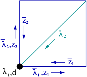
Figure 1: The lattice for pure $(2,2)$ gauge theory, from Ref. [26].

	$z_{1}$	$\kern 0.6pt\overline{\kern-0.6ptz\kern-0.6pt}\kern 0.6pt_{1}$	$z_{2}$	$\kern 0.6pt\overline{\kern-0.6ptz\kern-0.6pt}\kern 0.6pt_{2}$	$\lambda_{1}$	$\lambda_{2}$	$\kern 0.6pt\overline{\kern-0.6pt\lambda\kern-0.6pt}\kern 0.6pt_{1}$	$\kern 0.6pt\overline{\kern-0.6pt\lambda\kern-0.6pt}\kern 0.6pt_{2}$	$d$
$L_{3}$	$-{\textstyle{\frac{1}{2}}}$	$+{\textstyle{\frac{1}{2}}}$	$+{\textstyle{\frac{1}{2}}}$	$-{\textstyle{\frac{1}{2}}}$	$\,\ 0$	$\,\ 0$	$-{\textstyle{\frac{1}{2}}}$	$+{\textstyle{\frac{1}{2}}}$	$0$
$R_{3}$	$+{\textstyle{\frac{1}{2}}}$	$-{\textstyle{\frac{1}{2}}}$	$+{\textstyle{\frac{1}{2}}}$	$-{\textstyle{\frac{1}{2}}}$	$+{\textstyle{\frac{1}{2}}}$	$-{\textstyle{\frac{1}{2}}}$	$\,\ 0$	$\,\ 0$	$0$
$Y$	$\,\ 0$	$\,\ 0$	$\,\ 0$	$\,\ 0$	$+{\textstyle{\frac{1}{2}}}$	$+{\textstyle{\frac{1}{2}}}$	$-{\textstyle{\frac{1}{2}}}$	$-{\textstyle{\frac{1}{2}}}$	$0$
$r_{1}$	$+1$	$-1$	$\,\ 0$	$\,\ 0$	$\,\ 0$	$-1$	$+1$	$\,\ 0$	$0$
$r_{2}$	$\,\ 0$	$\,\ 0$	$+1$	$-1$	$\,\ 0$	$-1$	$\,\ 0$	$+1$	$0$

Table 1: The $r_{1,2}$ charges of the gauge multiplet.

The orbifold lattice construction technique also renders writing down the lattice action a simple mechanical exercise; here we summarize the results of Ref. [26]. The lattice variables in Fig. 1 are $k$ dimensional matrices, where Greek letters correspond to Grassmann variables, while Latin letters are bosons. The lattice action possesses a $U(k)$ gauge symmetry and single exact supercharge which can be realized as $Q=\partial/\partial\theta$, where $\theta$ is a Grassmann coordinate. To make the supersymmetry manifest, the variables are organized into superfields as

$$\mathbf{Z}_{i,{\bf n}} = z_{i,{\bf n}}+\sqrt{2}\,\theta\,\kern 0.6pt\overline{\kern-0.6pt\lambda\kern-0.6pt}\kern 0.6pt_{i,{\bf n}}$$ (5)

$$\bm{\Lambda}_{\bf n} = \lambda_{1,{\bf n}}+\theta\,\bigl{[}\left(z_{i,{\bf n}}\kern 0.6pt\overline{\kern-0.6ptz\kern-0.6pt}\kern 0.6pt_{i,{\bf n}}-\kern 0.6pt\overline{\kern-0.6ptz\kern-0.6pt}\kern 0.6pt_{i,{\bf n}-{\bf e}_{i}}z_{i,{\bf n}-{\bf e}_{i}}-id_{\bf n}\right)\bigr{]}$$ (6)

$$\bm{\Xi}_{ij,{\bf n}} = \lambda_{2,{\bf n}}\epsilon_{ij}+2\,\theta\left(\kern 0.6pt\overline{\kern-0.6ptz\kern-0.6pt}\kern 0.6pt_{i,{\bf n}+{\bf e}_{i}}\kern 0.6pt\overline{\kern-0.6ptz\kern-0.6pt}\kern 0.6pt_{j,{\bf n}}-\kern 0.6pt\overline{\kern-0.6ptz\kern-0.6pt}\kern 0.6pt_{j,{\bf n}+{\bf e}_{j}}\kern 0.6pt\overline{\kern-0.6ptz\kern-0.6pt}\kern 0.6pt_{i,{\bf n}}\right)\ ;$$ (7)

a sum over repeated $i$ indices being implied, where ${\bf n}$ is a lattice vector with integer components, and ${\bf e}_{i}$ is a unit vector in the $i$ direction. The $\kern 0.6pt\overline{\kern-0.6ptz\kern-0.6pt}\kern 0.6pt_{i}$ bosons are supersymmetric singlets. The lattice action may then be written in manifestly supersymmetric form:

$$S = \frac{1}{g^{2}}\sum_{{\bf n}}\int\!d\theta\,{\rm Tr\,}\biggl{[}{\textstyle{\frac{1}{2}}}\bm{\Lambda}_{\bf n}\partial_{\theta}\,\bm{\Lambda}_{\bf n}-\bm{\Xi}_{ij,{\bf n}}\mathbf{Z}_{i,{\bf n}}\mathbf{Z}_{j,{\bf n}+{\bf e}_{i}}$$ (9)

$$+\bm{\Lambda}_{\bf n}\left(\mathbf{Z}_{i,{\bf n}}\kern 0.6pt\overline{\kern-0.6ptz\kern-0.6pt}\kern 0.6pt_{i,{\bf n}}-\kern 0.6pt\overline{\kern-0.6ptz\kern-0.6pt}\kern 0.6pt_{i,{\bf n}-{\bf e}_{i}}\mathbf{Z}_{i,{\bf n}-{\bf e}_{i}}\right)\biggr{]}\ .$$

The continuum limit is defined by expanding about the point in moduli space $z_{i}=\kern 0.6pt\overline{\kern-0.6ptz\kern-0.6pt}\kern 0.6pt_{i}=(1/\sqrt{2}a){\bf 1}_{k}$, where ${\bf 1}_{k}$ is the $k$ dimensional unit matrix and $a$ is identified as the lattice spacing, and then taking $a\to 0$ with $L=Na$ and $g_{2}=ga$ held fixed. An additional soft supersymmetry breaking mass term

$$\delta S=\frac{1}{g^{2}}\sum_{\bf n}a^{2}\mu^{2}\left(\kern 0.6pt\overline{\kern-0.6ptz\kern-0.6pt}\kern 0.6pt_{i,{\bf n}}z_{i,{\bf n}}-\frac{1}{2a^{2}}\right)$$ (10)

may be introduced to the action in order to lift the degeneracy of the moduli and fix the vacuum expectation value of the gauge bosons. The mass parameter $\mu$ is chosen to scale as $\mu\sim 1/L$ so as to leave physical properties at length scales smaller than $1/\mu$ unaffected by this modification to the action. The lattice action has been shown to converge to the $(2,2)$ target theory eq. (2) with the lattice and continuum variables related as $z_{i}=\frac{1}{\sqrt{2}}\left(1/a+s_{i}+iv_{i}\right)$, where

$$s=\frac{s_{1}+is_{2}}{\sqrt{2}}\ ,\quad\Psi=\begin{pmatrix}\lambda_{1}\cr\lambda_{2}\end{pmatrix}\ ,\quad\kern 0.6pt\overline{\kern-0.6pt\Psi\kern-0.6pt}\kern 0.6pt=\begin{pmatrix}\kern 0.6pt\overline{\kern-0.6pt\lambda\kern-0.6pt}\kern 0.6pt_{1}&\kern 0.6pt\overline{\kern-0.6pt\lambda\kern-0.6pt}\kern 0.6pt_{2}\end{pmatrix}$$ (11)

in a particular basis for the Dirac $\gamma$ matrices [26].

3 Adjoint matter

We now turn to supersymmetric lattices for gauge theories with matter multiplets, once again employing the orbifold technique. To illustrate the general structure of these theories on the lattice, we first consider as our target theory a $(2,2)$ gauge theory with gauge group $G=U(k)$ (with $k=1$ a possibility) and $N_{f}$ flavors of adjoint matter fields. The parent theory is a four dimensional ${\cal N}=1$ theory with gauge group $\tilde{G}=U(kN^{2})$ and chiral superfields $\bm{\Phi}^{a}$, $a=1,\ldots,N_{f}$ transforming as adjoints under $\tilde{G}$, and a superpotential $W(\bm{\Phi})$ that preserves the $U(1)$ $R$-symmetry.

The orbifold projection of the matter fields follows a similar path from that outlined in the previous section for the gauge multiplet. Each chiral field $\bm{\Phi}$ from the parent theory contributes a boson $A$, auxiliary field $F$, and two component fermion $\psi_{i}$; $\kern 0.6pt\overline{\kern-0.6pt\bm{\Phi}\kern-0.6pt}\kern 0.6pt$ contributes barred versions of the same. Once again, the placement of these variables on the lattice is entirely dictated by their transformation properties under the global $SU(2)_{R}\times SU(2)_{L}\times U(1)$ symmetry of the parent theory, which we give in Table 2. An ambiguity is apparent in the assignment of the $U(1)$ symmetry to each field, and we have assigned in the parent theory a $U(1)$ charge $y$ to our generic $\bm{\Phi}$. Without a superpotential, there is freedom to assign to each chiral superfield an independent value for $y$; however, it is apparent from Table 2 that to obtain a sensible lattice with only nearest neighbor interactions (i.e. all $r_{i}$ charges equal to $0$ or $\pm 1$), we are constrained to choose $y=0$ or $y=1$. The result of this choice is shown in Fig. 2; in fact, we will need both types of matter multiplets, since the superpotential $W$ must have net charge $Y=1$.

	$A$	$\kern 0.6pt\overline{\kern-0.6ptA\kern-0.6pt}\kern 0.6pt$	$\psi_{1}$	$\psi_{2}$	$\kern 0.6pt\overline{\kern-0.6pt\psi\kern-0.6pt}\kern 0.6pt_{1}$	$\kern 0.6pt\overline{\kern-0.6pt\psi\kern-0.6pt}\kern 0.6pt_{2}$	$F$	$\kern 0.6pt\overline{\kern-0.6ptF\kern-0.6pt}\kern 0.6pt$
$L_{3}$	$\,\ 0$	$\,\ 0$	$\,\ 0$	$\,\ 0$	$-{\textstyle{\frac{1}{2}}}$	$+{\textstyle{\frac{1}{2}}}$	0	0
$R_{3}$	$\,\ 0$	$\,\ 0$	$+{\textstyle{\frac{1}{2}}}$	$-{\textstyle{\frac{1}{2}}}$	$\,\ 0$	$\,\ 0$	0	0
$Y$	$+y$	$-y$	$y-{\textstyle{\frac{1}{2}}}$	$y-{\textstyle{\frac{1}{2}}}$	$-y+{\textstyle{\frac{1}{2}}}$	$-y+{\textstyle{\frac{1}{2}}}$	$y-1$	$-y+1$
$r_{1}$	$-y$	$+y$	$1-y$	$-y$	$+y$	$-1+y$	$y-1$	$-y+1$
$r_{2}$	$-y$	$+y$	$1-y$	$-y$	$-1+y$	$+y$	$y-1$	$-y+1$

Table 2: The $r_{1,2}$ charges of the matter multiplet.

We can organize the chiral multiplet $\bm{\Phi}$ of the parent theory for either case $y=0,1$ into lattice superfields:

$${\bf A}_{\bf n} = A_{\bf n}+\sqrt{2}\theta\psi_{2,{\bf n}}$$ (12)

$${\mathbf{\Psi}}_{{\bf n}} = \psi_{1,{\bf n}}-\sqrt{2}\theta F_{\bf n}$$ (13)

$$\kern 0.6pt\overline{\kern-0.6pt{\mathbf{\Psi}}\kern-0.6pt}\kern 0.6pt_{i,{\bf n}} = \kern 0.6pt\overline{\kern-0.6pt\psi\kern-0.6pt}\kern 0.6pt_{i,{\bf n}}+2\theta\,\epsilon_{ij}(\kern 0.6pt\overline{\kern-0.6ptA\kern-0.6pt}\kern 0.6pt_{{\bf n}+{\bf e}_{j}}\kern 0.6pt\overline{\kern-0.6ptz\kern-0.6pt}\kern 0.6pt_{j,{\bf n}+y\,{\bf e}_{12}}-\kern 0.6pt\overline{\kern-0.6ptz\kern-0.6pt}\kern 0.6pt_{j,{\bf n}}\kern 0.6pt\overline{\kern-0.6ptA\kern-0.6pt}\kern 0.6pt_{\bf n})$$ (14)

$$\kern 0.6pt\overline{\kern-0.6pt\mathbf{F}\kern-0.6pt}\kern 0.6pt_{\bf n} = \kern 0.6pt\overline{\kern-0.6ptF\kern-0.6pt}\kern 0.6pt_{\bf n}-2\theta\,\biggl{(}\kern 0.6pt\overline{\kern-0.6ptA\kern-0.6pt}\kern 0.6pt_{{\bf n}+{\bf e}_{12}}\lambda_{2,{\bf n}+y\,{\bf e}_{12}}-\lambda_{2,{\bf n}}\kern 0.6pt\overline{\kern-0.6ptA\kern-0.6pt}\kern 0.6pt_{{\bf n}}$$ (16)

$$+\epsilon_{ij}\epsilon_{ik}\left[\kern 0.6pt\overline{\kern-0.6pt\psi\kern-0.6pt}\kern 0.6pt_{k,{\bf n}+{\bf e}_{j}}\kern 0.6pt\overline{\kern-0.6ptz\kern-0.6pt}\kern 0.6pt_{j,{\bf n}+y\,{\bf e}_{12}}-\kern 0.6pt\overline{\kern-0.6ptz\kern-0.6pt}\kern 0.6pt_{j,{\bf n}+{\bf e}_{i}}\kern 0.6pt\overline{\kern-0.6pt\psi\kern-0.6pt}\kern 0.6pt_{k,{\bf n}}\right]\biggr{)}$$

where ${\bf e}_{12}=({\bf e}_{1}+{\bf e}_{2})$ and $\kern 0.6pt\overline{\kern-0.6ptA\kern-0.6pt}\kern 0.6pt$ is a supersymmetric singlet. Note the appearance of $\lambda_{2}$ and $\kern 0.6pt\overline{\kern-0.6ptz\kern-0.6pt}\kern 0.6pt_{i}$ from the gauge supermultiplet eq. (7), which implies nontrivial consistency conditions which can be shown to hold. In the Appendix we make contact between the rather unfamiliar multiplet structure in eq. (16), and the more familiar chiral superfields from $N=1$ supersymmetry in the $3+1$ dimensional continuum.

In terms of the above fields, the orbifold projection of the parent theory produces the following lattice kinetic Lagrangian for the matter:

$${\cal L}_{\text{kin}} = \frac{1}{g^{2}}\int\!d\theta\,{\rm Tr\,}\big{[}\epsilon_{ij}\kern 0.6pt\overline{\kern-0.6pt{\mathbf{\Psi}}\kern-0.6pt}\kern 0.6pt_{i,{\bf n}}\left(\mathbf{Z}_{j,{\bf n}+y\,{\bf e}_{12}}{\bf A}_{{\bf n}+{\bf e}_{j}}-{\bf A}_{\bf n}\mathbf{Z}_{j,{\bf n}}\right)$$ (18)

$$+\kern 0.6pt\overline{\kern-0.6ptA\kern-0.6pt}\kern 0.6pt_{\bf n}\left(\bm{\Lambda}_{{\bf n}+y\,{\bf e}_{12}}{\bf A}_{\bf n}-{\bf A}_{\bf n}\bm{\Lambda}_{\bf n}\right)-\frac{1}{\sqrt{2}}\kern 0.6pt\overline{\kern-0.6pt\mathbf{F}\kern-0.6pt}\kern 0.6pt_{\bf n}{\mathbf{\Psi}}_{\bf n}\big{]}\ .$$

The superpotential contributions for the theory are

$${\cal L}_{W} = \frac{1}{g^{2}}{\rm Tr\,}\biggl{[}\left(\int\!d\theta\,\frac{1}{\sqrt{2}}{\mathbf{\Psi}}^{a}W_{a}({\bf A})\right)+\kern 0.6pt\overline{\kern-0.6pt\mathbf{F}\kern-0.6pt}\kern 0.6pt^{a}\kern 0.6pt\overline{\kern-0.6ptW\kern-0.6pt}\kern 0.6pt_{a}(\kern 0.6pt\overline{\kern-0.6ptA\kern-0.6pt}\kern 0.6pt)-\kern 0.6pt\overline{\kern-0.6pt{\mathbf{\Psi}}\kern-0.6pt}\kern 0.6pt_{1}^{a}\kern 0.6pt\overline{\kern-0.6pt{\mathbf{\Psi}}\kern-0.6pt}\kern 0.6pt_{2}^{b}\kern 0.6pt\overline{\kern-0.6ptW\kern-0.6pt}\kern 0.6pt_{ab}(\kern 0.6pt\overline{\kern-0.6ptA\kern-0.6pt}\kern 0.6pt)\biggr{]}$$ (19)

where $W({\bf A})$ is a polynomial in the ${\bf A}$ fields with $R$-charge $y=1$ (and $\kern 0.6pt\overline{\kern-0.6ptW\kern-0.6pt}\kern 0.6pt(\kern 0.6pt\overline{\kern-0.6ptA\kern-0.6pt}\kern 0.6pt)$ is its conjugate), while $W_{a}=\partial W/\partial A^{a}$ and $W_{ab}=\partial^{2}W/\partial A^{a}\partial A^{b}$. The space-time dependence has been omitted as it is implied by the gauge invariance of the Lagrangian; each term in the superpotential should form a closed loop on the space-time lattice. One can verify by explicit calculation that the $\theta$ dependence cancels between the second and third terms after summing over lattice sites, and therefore the action is annihilated by $Q=\partial/\partial\theta$ and is supersymmetric.

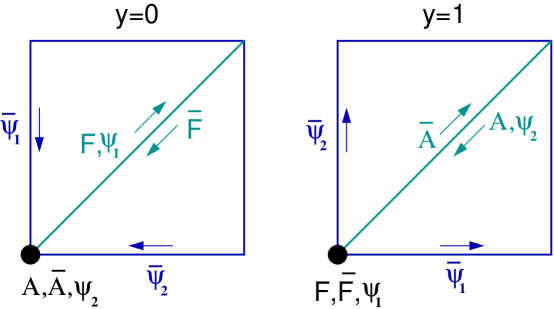
Figure 2: Placement of the matter variables within the unit cell for the two choices $y=0$ and $y=1$ for the $U(1)$ $R$-charge.

As an example of how to interpret the above terms, we consider a two flavor model ($N_{f}=2$) and the superpotential $W(\bm{\Phi})=c\,{\rm Tr\,}\bm{\Phi}^{1}\bm{\Phi}^{2}$. The superpotential must carry charge $Y=1$, which can be satisfied by choosing for the superfields $R$-charges $y_{1}=1$ and $y_{2}=0$ for $\bm{\Phi}^{1}$ and $\bm{\Phi}^{2}$ respectively. These charge assignments dictate the lattice representation for these superfields, as shown in Fig. 2. The first term in eq. (19), for example, is then

$${\rm Tr\,}{\mathbf{\Psi}}^{a}W_{a}({\bf A}) = c\,{\rm Tr\,}\left({\mathbf{\Psi}}^{1}_{{\bf n}}{\bf A}^{2}_{{\bf n}}+{\bf A}^{1}_{{\bf n}}{\mathbf{\Psi}}^{2}_{{\bf n}}\right)$$ (20)

which is seen to be gauge invariant since $\{{\bf A}^{1},{\mathbf{\Psi}}^{1}\}$ are $\{-\text{diagonal, site}\}$ variables, while $\{{\bf A}^{2},{\mathbf{\Psi}}^{2}\}$ are $\{\text{site, +diagonal}\}$ variables.

The continuum limit of the above theory is defined as in the previous section for the pure gauge theory, and the desired $(2,2)$ theory with matter results at the classical level. An analysis of the continuum limit, including quantum corrections can be found in the Appendix. In the case $k=1$, the continuum gauge symmetry is $U(1)$ and one obtains a theory of neutral matter interacting via a superpotential.

4 More general matter multiplets

More general theories of matter fields interacting via gauge interactions and a superpotential may be obtained by orbifolding the parent theory of §3 by some $N$-independent discrete symmetry, before orbifolding by $Z_{N}\times Z_{N}$. Here we give several examples.

Example 1: $SU(2)\times U(1)$ with charged doublets. Consider the parent theory with a $U(3N^{2})$ gauge symmetry, adjoint superfields $\bm{\Phi}^{1}$ and $\bm{\Phi}^{2}$, and the superpotential $W(\bm{\Phi})=c\,{\rm Tr\,}\bm{\Phi}^{1}\bm{\Phi}^{1}\bm{\Phi}^{2}$. Here, we choose $y_{1}=0$ and $y_{2}=1$ as R-charges for our superfields. This theory has a $\bm{\Phi}^{a}\to(-1)^{a}\bm{\Phi}^{a}$ symmetry, and so we can impose the additional orbifold condition $P\bm{\Phi}^{a}P=(-1)^{a}\bm{\Phi}^{a}$ and $P\mathbf{V}P=\mathbf{V}$ where $\mathbf{V}$ is the vector supermultiplet of the parent theory and $P$ is a $U(3N^{2})$ matrix with $\{1,1,-1\}$ along the diagonal, where each entry is an $N^{2}$ dimensional unit matrix. This projection breaks the $U(3N^{2})$ gauge symmetry down to $U(2N^{2})\times U(N^{2})$, under which the projected matter field $\bm{\Phi}^{1}$ decomposes as $(\raisebox{-0.5pt}{\hbox{\rule{0.4pt}{6.5pt}\hskip-0.4pt\rule{6.5pt}{0.4pt}\hskip-6.5pt\rule[6.5pt]{6.5pt}{0.4pt}}\rule[6.5pt]{0.4pt}{0.4pt}\hskip-0.4pt\rule{0.4pt}{6.5pt}},\kern 0.6pt\overline{\kern-0.6pt\raisebox{-0.5pt}{\hbox{\rule{0.4pt}{6.5pt}\hskip-0.4pt\rule{6.5pt}{0.4pt}\hskip-6.5pt\rule[6.5pt]{6.5pt}{0.4pt}}\rule[6.5pt]{0.4pt}{0.4pt}\hskip-0.4pt\rule{0.4pt}{6.5pt}}\kern-0.6pt}\kern 0.6pt)\oplus(\kern 0.6pt\overline{\kern-0.6pt\raisebox{-0.5pt}{\hbox{\rule{0.4pt}{6.5pt}\hskip-0.4pt\rule{6.5pt}{0.4pt}\hskip-6.5pt\rule[6.5pt]{6.5pt}{0.4pt}}\rule[6.5pt]{0.4pt}{0.4pt}\hskip-0.4pt\rule{0.4pt}{6.5pt}}\kern-0.6pt}\kern 0.6pt,\raisebox{-0.5pt}{\hbox{\rule{0.4pt}{6.5pt}\hskip-0.4pt\rule{6.5pt}{0.4pt}\hskip-6.5pt\rule[6.5pt]{6.5pt}{0.4pt}}\rule[6.5pt]{0.4pt}{0.4pt}\hskip-0.4pt\rule{0.4pt}{6.5pt}})$ and $\bm{\Phi}^{2}$ decomposes as $({\bf adj},1)\oplus(1,{\bf adj})$. We then orbifold the parent theory by $Z_{N}\times Z_{N}$, resulting in a lattice with an $SU(2)\times U(1)\times U(1)$ gauge theory, with matter multiplets transforming as $3_{0,0}\oplus 2_{\pm 1/2,0}\oplus 1_{0,0}\oplus 1_{0,0}$ in the continuum limit. The doublet couples to both the triplet and one of the singlets in the superpotential. Evidently the second $U(1)$ gauge sector decouples from the theory since no fields carry that charge.

It is possible to generalize the above construction to fundamental matter transforming as $\raisebox{-0.5pt}{\hbox{\rule{0.4pt}{6.5pt}\hskip-0.4pt\rule{6.5pt}{0.4pt}\hskip-6.5pt\rule[6.5pt]{6.5pt}{0.4pt}}\rule[6.5pt]{0.4pt}{0.4pt}\hskip-0.4pt\rule{0.4pt}{6.5pt}}_{+1}\oplus\kern 0.6pt\overline{\kern-0.6pt\raisebox{-0.5pt}{\hbox{\rule{0.4pt}{6.5pt}\hskip-0.4pt\rule{6.5pt}{0.4pt}\hskip-6.5pt\rule[6.5pt]{6.5pt}{0.4pt}}\rule[6.5pt]{0.4pt}{0.4pt}\hskip-0.4pt\rule{0.4pt}{6.5pt}}\kern-0.6pt}\kern 0.6pt_{-1}$ under $SU(M)\times U(1)$ gauge transformations by starting with a $U((M+1)N^{2})$ theory broken down to $U(MN^{2})\times U(N^{2})$.

Example 2: $U(1)^{k}$ quiver with Fayet-Iliopoulos terms. A different sort of theory may be obtained by considering a parent theory with a $U(kN^{2})$ gauge symmetry and a single matter adjoint $\bm{\Phi}$ with a superpotential $W(\bm{\Phi})=c/k{\rm Tr\,}\bm{\Phi}^{k}$. The initial orbifold condition is $\mathbf{V}=P\mathbf{V}P^{\dagger}$ and $\bm{\Phi}=\omega P\bm{\Phi}P^{\dagger}$ on the parent theory, where $\omega=exp(i2\pi/k)$ and $P$ is the diagonal $kN^{2}$ dimensional “clock” matrix $\text{diag}\{1,\omega,\omega^{2}\ldots,\omega^{k-1}\}$, each entry appearing $N^{2}$ times. This projection produces a quiver theory, breaking the gauge symmetry down from $U(kN^{2})$ to $U(N^{2})^{k}$, and producing bifundamental matter fields $\bm{\Phi}^{a}$, with $a=1,\ldots,k$ transforming as $(\raisebox{-0.5pt}{\hbox{\rule{0.4pt}{6.5pt}\hskip-0.4pt\rule{6.5pt}{0.4pt}\hskip-6.5pt\rule[6.5pt]{6.5pt}{0.4pt}}\rule[6.5pt]{0.4pt}{0.4pt}\hskip-0.4pt\rule{0.4pt}{6.5pt}},\kern 0.6pt\overline{\kern-0.6pt\raisebox{-0.5pt}{\hbox{\rule{0.4pt}{6.5pt}\hskip-0.4pt\rule{6.5pt}{0.4pt}\hskip-6.5pt\rule[6.5pt]{6.5pt}{0.4pt}}\rule[6.5pt]{0.4pt}{0.4pt}\hskip-0.4pt\rule{0.4pt}{6.5pt}}\kern-0.6pt}\kern 0.6pt)$ under $G_{a}\times G_{a+1}$, where $G_{a}=U(N^{2})$ and $G_{k+1}\equiv G_{1}$. The superpotential becomes $W(\bm{\Phi})=c{\rm Tr\,}\bm{\Phi}^{1}\cdots\bm{\Phi}^{k}$.

One can assign $y=1$ to one of the $k$ matter fields, and $y=0$ to the others. A subsequent $Z_{N}\times Z_{N}$ projection then produces a lattice theory with a $U(1)^{k}$ gauge symmetry, where the descendants of the parent multiplet $\bm{\Phi}^{a}$ carry $U(1)$ charges $q_{b}=(\delta_{ab}-\delta_{a,b-1})$, with $q_{k+1}\equiv q_{1}$. One can also add Fayet-Iliopoulos terms to the action given by $-i\xi\,\int d\theta\,\sum_{\bf n}\,{\rm Tr\,}\bm{\Lambda}^{a}_{\bf n}$, as is apparent from eq. (7). Such a theory is directly related to Calabi-Yau manifolds, as discussed in [34], and would be interesting to study numerically.

It should be apparent that although we focused on a $U(1)^{k}$ quiver, any $U(p)^{q}$ quiver can be constructed in a similar manner. We have not found a way to construct lattices for arbitrary matter representations.

Appendix A Superfield structure

The relationship between the lattice superfields defined in eq. (16) and the continuum chiral superfields of the parent theory can be most easily seen if we turn off the gauge interactions. Consider the familiar superfield formulation of ${\cal N}=1$ supersymmetry in four dimensions. We work in the superspace coordinate basis $(y,\,\theta,\,\kern 0.6pt\overline{\kern-0.6pt\theta\kern-0.6pt}\kern 0.6pt)$ from ref. [35], where $\theta$ is a two-component complex Grassmann spinor, and $y_{m}\equiv(x_{m}+i\theta\sigma_{m}\kern 0.6pt\overline{\kern-0.6pt\theta\kern-0.6pt}\kern 0.6pt)$. In this basis the chiral supercharges $Q_{\alpha}$ are particularly simple,

$$Q_{\alpha}=\frac{\partial\ }{\partial\theta^{\alpha}}\ .$$ (21)

Furthermore, a chiral superfield $\bm{\Phi}(y,\theta)$ is independent of $\kern 0.6pt\overline{\kern-0.6pt\theta\kern-0.6pt}\kern 0.6pt$ in this basis, and may be decomposed as

$$\bm{\Phi} = A(y)+\sqrt{2}\theta\psi(y)+\theta\theta F(y)$$ (22)

$$= {\bf A}(y,\theta^{2})+\sqrt{2}\theta^{1}{\mathbf{\Psi}}(y,\theta^{2})\ ,$$ (23)

where we follow the spinor notation of [35], and ${\bf A}$ and ${\mathbf{\Psi}}$ are defined as

$${\bf A} = A(y)+\sqrt{2}\,\theta^{2}\psi_{2}(y)\ ,$$ (24)

$${\mathbf{\Psi}} = \psi_{1}(y)-\sqrt{2}\,\theta^{2}F(y)\ .$$ (25)

We see that ${\bf A}$ and ${\mathbf{\Psi}}$ correspond to the first two lattice multiplets in eq. (16), where the surviving lattice supersymmetry generator is $Q_{2}=\partial/\partial\theta^{2}$.

The anti-chiral superfield in four dimensions may be written as $\kern 0.6pt\overline{\kern-0.6pt\bm{\Phi}\kern-0.6pt}\kern 0.6pt(\kern 0.6pt\overline{\kern-0.6pty\kern-0.6pt}\kern 0.6pt,\kern 0.6pt\overline{\kern-0.6pt\theta\kern-0.6pt}\kern 0.6pt)$. When this is converted to the $(y,\,\theta,\,\kern 0.6pt\overline{\kern-0.6pt\theta\kern-0.6pt}\kern 0.6pt)$ basis, $\kern 0.6pt\overline{\kern-0.6pt\bm{\Phi}\kern-0.6pt}\kern 0.6pt$ has the expansion

$$\kern 0.6pt\overline{\kern-0.6pt\bm{\Phi}\kern-0.6pt}\kern 0.6pt = \kern 0.6pt\overline{\kern-0.6ptA\kern-0.6pt}\kern 0.6pt(\kern 0.6pt\overline{\kern-0.6pty\kern-0.6pt}\kern 0.6pt)+\sqrt{2}\kern 0.6pt\overline{\kern-0.6pt\theta\kern-0.6pt}\kern 0.6pt\kern 0.6pt\overline{\kern-0.6pt\psi\kern-0.6pt}\kern 0.6pt(\kern 0.6pt\overline{\kern-0.6pty\kern-0.6pt}\kern 0.6pt)+\kern 0.6pt\overline{\kern-0.6pt\theta\kern-0.6pt}\kern 0.6pt\kern 0.6pt\overline{\kern-0.6pt\theta\kern-0.6pt}\kern 0.6pt\kern 0.6pt\overline{\kern-0.6ptF\kern-0.6pt}\kern 0.6pt(\kern 0.6pt\overline{\kern-0.6pty\kern-0.6pt}\kern 0.6pt)$$ (26)

$$= \kern 0.6pt\overline{\kern-0.6ptA\kern-0.6pt}\kern 0.6pt(y)-\sqrt{2}\kern 0.6pt\overline{\kern-0.6pt\theta\kern-0.6pt}\kern 0.6pt^{j}\left[\kern 0.6pt\overline{\kern-0.6pt{\mathbf{\Psi}}\kern-0.6pt}\kern 0.6pt_{j}(y,\theta^{2})+\sqrt{2}\theta^{1}\partial_{j}\kern 0.6pt\overline{\kern-0.6ptA\kern-0.6pt}\kern 0.6pt(y)\right]$$ (29)

$$+\kern 0.6pt\overline{\kern-0.6pt\theta\kern-0.6pt}\kern 0.6pt\kern 0.6pt\overline{\kern-0.6pt\theta\kern-0.6pt}\kern 0.6pt\left[\kern 0.6pt\overline{\kern-0.6pt\mathbf{F}\kern-0.6pt}\kern 0.6pt(y,\theta^{2})-\sqrt{2}\theta^{1}\epsilon_{ij}\partial_{i}\kern 0.6pt\overline{\kern-0.6pt{\mathbf{\Psi}}\kern-0.6pt}\kern 0.6pt_{j}(y,\theta^{2})\right]\ ,$$

where

$$\kern 0.6pt\overline{\kern-0.6pt{\mathbf{\Psi}}\kern-0.6pt}\kern 0.6pt_{i} = \kern 0.6pt\overline{\kern-0.6pt\psi\kern-0.6pt}\kern 0.6pt_{i}(y)+\sqrt{2}\theta^{2}\epsilon_{ij}\partial_{j}\kern 0.6pt\overline{\kern-0.6ptA\kern-0.6pt}\kern 0.6pt(y)\ ,$$ (30)

$$\kern 0.6pt\overline{\kern-0.6pt\mathbf{F}\kern-0.6pt}\kern 0.6pt = \kern 0.6pt\overline{\kern-0.6ptF\kern-0.6pt}\kern 0.6pt(y)-\sqrt{2}\theta^{2}\partial_{j}\kern 0.6pt\overline{\kern-0.6pt\psi\kern-0.6pt}\kern 0.6pt_{j}(y)\ .$$ (31)

The multiplets $\kern 0.6pt\overline{\kern-0.6pt{\mathbf{\Psi}}\kern-0.6pt}\kern 0.6pt_{i}$ and $\kern 0.6pt\overline{\kern-0.6pt\mathbf{F}\kern-0.6pt}\kern 0.6pt$ are just the continuum versions of the second two supermultiplets in eq. (16), after replacing $\theta\to\theta^{2}$ and setting to zero the gauge and gaugino fields. Note that the lattice supercharge we have constructed is gauge invariant, which is why the gauge and gaugino fields appear in our lattice superfields.

With the above packaging, the kinetic energy and superpotential terms for matter in the lattice theory coincide with those of the parent theory. For example, ${\cal L}_{\text{kin}}$ in eq. (18) takes the familiar form

$${\cal L}_{\text{kin}} = \frac{1}{4}\int\!d\theta^{2}\,d\theta^{1}\,d\kern 0.6pt\overline{\kern-0.6pt\theta\kern-0.6pt}\kern 0.6pt^{1}\,d\kern 0.6pt\overline{\kern-0.6pt\theta\kern-0.6pt}\kern 0.6pt^{2}\,\kern 0.6pt\overline{\kern-0.6pt\bm{\Phi}\kern-0.6pt}\kern 0.6pt\bm{\Phi}\ .$$ (32)

Appendix B Continuum limit and renormalization

Radiative corrections and renormalization for the pure (2,2) gauge theory were considered in Ref. [26]; here we extend that analysis to include the matter fields interacting through a superpotential

$$W={\rm Tr\,}\left(\kappa_{2}^{A}\bm{\Phi}^{A}+\kappa_{1}^{Ab}\bm{\Phi}^{A}\bm{\Phi}^{b}+\kappa_{0}^{Abc}\bm{\Phi}^{A}\bm{\Phi}^{b}\bm{\Phi}^{c}\right)$$ (33)

where the index $A$ sums over all flavors of $y=1$ matter fields, while $b$, $c$ sum over $y=0$ matter fields (we have normalized the $R$-symmetry such that $W$ has $y=1$).

Induced operators in the Symanzik action take the form

$$\delta S_{\cal O}=\frac{1}{g_{2}^{2}}\int\!d^{2}z\,C_{\cal O}{\cal O}\ ,$$ (34)

where ${\cal O}$ is a local operator in the continuum, and $C_{\cal O}$ is a coefficient depending on the lattice spacing $a$. The super-renormalizability of the target theory is most easily accounted for by defining the scaling dimension of ${\cal O}$ according to the usual conventions of four dimensional theories: bosons have mass dimension 1, fermions have mass dimension 3/2, $z$ and $\theta$ have mass dimension $-1$ and $-{\textstyle{\frac{1}{2}}}$ respectively. Then for an operator ${\cal O}$ of dimension $p$, the coefficient $C_{\cal O}$ induced by radiative corrections takes the form

$$C_{\cal O}=a^{p-4}\sum_{\ell=1}^{\infty}c_{\ell}(g_{2}^{2}a^{2})^{\ell}\times F_{\ell}(\kappa_{0},a\kappa_{1},a^{2}\kappa_{2})\ ,$$ (35)

where $\ell$ corresponds to the number of loops in a perturbative expansion, and $c_{\ell}$ is a dimensionless coefficient with only possible logarithmic dependence on $a$. The functions $F_{\ell}$ may depend on both $\kappa_{n}$ and $\kern 0.6pt\overline{\kern-0.6pt\kappa\kern-0.6pt}\kern 0.6pt_{n}$, but will not diverge as inverse powers of $a$ as $a\to 0$.

Induced operators with coefficients which do not vanish as $a\to 0$ will typically spoil the continuum limit of the theory. However we see that these could only correspond to $p=2$ at $\ell=1$, $p=1$ at $\ell=1$, or $p=0$ at $\ell=1,2$. We can ignore the $p=0$ case, which corresponds to a cosmological constant and has no noticeable effects on the continuum limit. That leaves us with the only operators to consider being dimension $p=1$ (scalar tadpole) or $p=2$ (scalar mass or $F$ tadpole). These operators must be consistent with the exact symmetries of the lattice: (i) ${\cal Q}=1$ supersymmetry; (ii) the $Z_{2}$ reflection symmetry about the diagonal link; (iii) gauge symmetry; (iv) $U(1)$ symmetries. The latter include not only the exact $U(1)^{3}$ global symmetry corresponding to $r_{1}$, $r_{2}$ and $y$, but also the approximate $U(1)^{2}$ symmetry broken by the superpotential under which the $\kappa_{n}$ act as spurions:

$$\bm{\Phi}^{a}\to e^{i\alpha}\bm{\Phi}^{a}\ ,\ \ \bm{\Phi}^{A}\to e^{i\beta}\bm{\Phi}^{A}\ ,\ \ \kappa_{0}\to e^{-i(2\alpha+\beta)}\kappa_{0}\ ,\ \ \kappa_{1}\to e^{-i(\alpha+\beta)}\kappa_{1}\ ,\ \ \kappa_{2}\to e^{-i\beta}\kappa_{2}\ .$$ (36)

(37)

There may be additional symmetries restricting the form of counterterms, depending on the form of $W$.

At $p=2$ the operators allowed by symmetry are

$$\int\!d\theta{\rm Tr\,}{\mathbf{\Psi}}^{A}\ ,\qquad{\rm Tr\,}\kern 0.6pt\overline{\kern-0.6pt\mathbf{F}\kern-0.6pt}\kern 0.6pt^{A}\ ,\qquad{\rm Tr\,}\kern 0.6pt\overline{\kern-0.6ptA\kern-0.6pt}\kern 0.6pt^{a}\kern 0.6pt\overline{\kern-0.6ptA\kern-0.6pt}\kern 0.6pt^{b}\ .$$ (38)

The second operator does not look supersymmetric, but one can verify that its $\theta$ component is a total derivative and makes no contribution to the action. In each of the above cases it is evident that the $U(1)^{2}$ symmetry of eq. (37) mandates powers of $a\kappa_{1}$ and/or $a^{2}\kappa_{2}$ in the operator coefficient $C_{\cal O}$, rendering each of these operators innocuous in the $a\to 0$ continuum limit.

At $p=1$ there exists a single operator allowed by the symmetries,

$${\rm Tr\,}\,\kern 0.6pt\overline{\kern-0.6ptA\kern-0.6pt}\kern 0.6pt^{a}\ ,$$ (39)

which might be induced at one loop with a coefficient $C_{\cal O}\propto g_{2}^{2}\kern 0.6pt\overline{\kern-0.6pt\kappa\kern-0.6pt}\kern 0.6pt_{0}^{Aab}\kappa_{1}^{Ab}$ times a possible log. This contribution can either be calculated and cancelled off by introducing an explicit tadpole term to the lattice action, or it may be forbidden by introducing a discrete $\bm{\Phi}^{a}\to-\bm{\Phi}^{a}$ symmetry, eliminating the $\kappa_{1}$ coefficient in the superpotential. In either case, the continuum theory can be attained without any numerical fine-tuning.

References

• [1] S. Catterall, Dirac-kaehler fermions and exact lattice supersymmetry, PoS LAT2005 (2005) 006, [hep-lat/0509136].
• [2] A. Feo, Supersymmetry on the lattice, Nucl. Phys. Proc. Suppl. 119 (2003) 198–209, [hep-lat/0210015].
• [3] J. W. Elliott and G. D. Moore, Three dimensional n = 2 supersymmetry on the lattice, PoS LAT2005 (2005) 245, [hep-lat/0509032].
• [4] J. Giedt, Deconstruction and other approaches to supersymmetric lattice field theories, Int. J. Mod. Phys. A21 (2006) 3039–3094, [hep-lat/0602007].
• [5] J. M. Rabin, Homology theory of lattice fermion doubling, Nucl. Phys. B201 (1982) 315.
• [6] P. Becher and H. Joos, The dirac-kahler equation and fermions on the lattice, Zeit. Phys. C15 (1982) 343.
• [7] S. Catterall and S. Karamov, Exact lattice supersymmetry: the two-dimensional n = 2 wess-zumino model, Phys. Rev. D65 (2002) 094501, [hep-lat/0108024].
• [8] S. Catterall and S. Karamov, A two-dimensional lattice model with exact supersymmetry, Nucl. Phys. Proc. Suppl. 106 (2002) 935–937, [hep-lat/0110071].
• [9] S. Catterall and S. Ghadab, Lattice sigma models with exact supersymmetry, JHEP 05 (2004) 044, [hep-lat/0311042].
• [10] S. Catterall, Lattice supersymmetry and topological field theory, JHEP 05 (2003) 038, [hep-lat/0301028].
• [11] F. Sugino, A lattice formulation of super yang-mills theories with exact supersymmetry, JHEP 01 (2004) 015, [hep-lat/0311021].
• [12] S. Catterall, A geometrical approach to n = 2 super yang-mills theory on the two dimensional lattice, JHEP 11 (2004) 006, [hep-lat/0410052].
• [13] J. Giedt, R-symmetry in the q-exact (2,2) 2d lattice wess-zumino model, Nucl. Phys. B726 (2005) 210–232, [hep-lat/0507016].
• [14] S. Catterall, Lattice formulation of n = 4 super yang-mills theory, JHEP 06 (2005) 027, [hep-lat/0503036].
• [15] S. Catterall, Simulations of n = 2 super yang-mills theory in two dimensions, JHEP 03 (2006) 032, [hep-lat/0602004].
• [16] F. Sugino, Two-dimensional compact n = (2,2) lattice super yang-mills theory with exact supersymmetry, Phys. Lett. B635 (2006) 218–224, [hep-lat/0601024].
• [17] S. Elitzur, E. Rabinovici, and A. Schwimmer, Supersymmetric models on the lattice, Phys. Lett. B119 (1982) 165.
• [18] N. Kawamoto and T. Tsukioka, N = 2 supersymmetric model with dirac-kaehler fermions from generalized gauge theory in two dimensions, Phys. Rev. D61 (2000) 105009, [hep-th/9905222].
• [19] J. Kato, N. Kawamoto, and Y. Uchida, Twisted superspace for n = d = 2 super bf and yang-mills with dirac-kaehler fermion mechanism, Int. J. Mod. Phys. A19 (2004) 2149–2182, [hep-th/0310242].
• [20] A. D’Adda, I. Kanamori, N. Kawamoto, and K. Nagata, Twisted superspace on a lattice, Nucl. Phys. B707 (2005) 100–144, [hep-lat/0406029].
• [21] J. Kato, N. Kawamoto, and A. Miyake, N = 4 twisted superspace from dirac-kaehler twist and off- shell susy invariant actions in four dimensions, Nucl. Phys. B721 (2005) 229–286, [hep-th/0502119].
• [22] A. D’Adda, I. Kanamori, N. Kawamoto, and K. Nagata, Exact extended supersymmetry on a lattice: Twisted n = 2 super yang-mills in two dimensions, Phys. Lett. B633 (2006) 645–652, [hep-lat/0507029].
• [23] F. Bruckmann and M. de Kok, Noncommutativity approach to supersymmetry on the lattice: Susy quantum mechanics and an inconsistency, Phys. Rev. D73 (2006) 074511, [hep-lat/0603003].
• [24] N. Arkani-Hamed, A. G. Cohen, D. B. Kaplan, A. Karch, and L. Motl, Deconstructing (2,0) and little string theories, JHEP 01 (2003) 083, [hep-th/0110146].
• [25] D. B. Kaplan, E. Katz, and M. Unsal, Supersymmetry on a spatial lattice, JHEP 05 (2003) 037, [hep-lat/0206019].
• [26] A. G. Cohen, D. B. Kaplan, E. Katz, and M. Unsal, Supersymmetry on a euclidean spacetime lattice. i: A target theory with four supercharges, JHEP 08 (2003) 024, [hep-lat/0302017].
• [27] A. G. Cohen, D. B. Kaplan, E. Katz, and M. Unsal, Supersymmetry on a euclidean spacetime lattice. ii: Target theories with eight supercharges, JHEP 12 (2003) 031, [hep-lat/0307012].
• [28] J. Giedt, E. Poppitz, and M. Rozali, Deconstruction, lattice supersymmetry, anomalies and branes, JHEP 03 (2003) 035, [hep-th/0301048].
• [29] J. Giedt, Non-positive fermion determinants in lattice supersymmetry, Nucl. Phys. B668 (2003) 138–150, [hep-lat/0304006].
• [30] J. Giedt and E. Poppitz, Lattice supersymmetry, superfields and renormalization, JHEP 09 (2004) 029, [hep-th/0407135].
• [31] D. B. Kaplan and M. Unsal, A euclidean lattice construction of supersymmetric yang- mills theories with sixteen supercharges, JHEP 09 (2005) 042, [hep-lat/0503039].
• [32] N. Arkani-Hamed, A. G. Cohen, and H. Georgi, (de)constructing dimensions, Phys. Rev. Lett. 86 (2001) 4757–4761, [http://arXiv.org/abs/hep-th/0104005].
• [33] M. Unsal, Twisted supersymmetric gauge theories and orbifold lattices, hep-th/0603046.
• [34] E. Witten, Phases of n = 2 theories in two dimensions, Nucl. Phys. B403 (1993) 159–222, [hep-th/9301042].
• [35] J. Wess and J. Bagger, Supersymmetry and supergravity, . Princeton, USA: Univ. Pr. (1992) 259 p.