Deconfinement in dense 2-color QCD

Abstract

We study SU(2) lattice gauge theory with two flavors of Wilson fermion at non-zero chemical potential $\mu$ and low temperature on a $8^{3}\times 16$ system. We identify three régimes along the $\mu$-axis. For $\mu\lesssim m_{\pi}/2$ the system remains in the vacuum phase, and all physical observables considered remain essentially unchanged. The intermediate régime is characterised by a non-zero diquark condensate and an associated increase in the baryon density, consistent with what is expected for Bose–Einstein condensation of tightly bound diquarks. We also observe screening of the static quark potential here. In the high-density deconfined régime we find a non-zero Polyakov loop and a strong modification of the gluon propagator, including significant screening in the magnetic sector in the static limit, which must have a non-perturbative origin. The behaviour of thermodynamic observables and the superfluid order parameter are consistent with a Fermi surface disrupted by a BCS diquark condensate. The energy per baryon as a function of $\mu$ exhibits a minimum in the deconfined régime, implying that macroscopic objects such as stars formed in this theory are largely composed of quark matter.

1 Introduction

At large quark chemical potential $\mu$, QCD is expected to undergo a transition from a confined nuclear matter phase to a deconfined quark matter phase, where the relevant degrees of freedom are quarks and gluons. It is now also generally believed that the quark matter phase at low temperature $T$ is characterised by diquark condensation: pairing of quarks near the Fermi surface gives rise to a number of color superconducting phases Rajagopal:2000wf ; Alford:2001dt ; Schafer:2003vz ; Shovkovy:2004me . The phase structure depends critically on the precise values of the diquark gap parameters and the effective strange quark mass at the relevant densities, and in the absence of a first-principles non-perturbative determination of these quantities, our knowledge of this region of the phase diagram will remain unsatisfactory.

Lattice QCD is at present unable to address these problems directly, since the fermion determinant is no longer positive definite once $\mu\neq 0$, and cannot be used as a probability weight in the functional integral. There has been much progress in recent years in developing methods for the region of high $T$, low $\mu$, where the problem is less severe Philipsen:2005mj . These methods are being extended in the direction of higher $\mu$ and lower $T$, but it is not clear at what point they break down, beyond which only unphysical results will be obtained.

Another approach is to study QCD-like theories where the fermion determinant remains real and positive even when $\mu\neq 0$. These can be used as a laboratory for investigating gauge theories at high density and low temperature. One such theory is 2-color QCD (QC₂D) with an even number of flavors Hands:1999md , where the quarks and antiquarks live in equivalent representations of the color group and can be related by an anti-unitary symmetry (the Pauli–Gürsey symmetry). This theory has been studied on the lattice by a number of groups Hands:1999md ; Aloisio:2000if ; Hands:2000ei ; Hands:2001ee ; Kogut:2002cm ; Muroya:2002ry ; Alles:2006ea ; Chandrasekharan:2006tz .

At $\mu=0$, the Pauli–Gürsey symmetry implies an exact symmetry between mesons and diquarks, which are the baryons of the theory. In particular, chiral multiplets will contain both mesons and baryons. For $N_{f}=2$ for example, the pseudo-Goldstone multiplet consists of the pion isotriplet plus a scalar isoscalar diquark and antidiquark. The diquark baryons can be expected to condense when $\mu\gtrsim m_{\pi}/2$, forming a superfluid ground state. In this respect, the theory is radically different from real QCD, where no gauge invariant diquark operator exists and the ground state at high density is superconducting. The nature of the superfluid ground state is however an interesting issue in its own right. For instance, an alternative approach to a superfluid order parameter in terms of an orthodox BCS description of diquark pairing at the Fermi surface has been given in Kondratyuk:1991hf .

In the gluon sector, the differences between SU(2) and SU(3) are expected to be less important, and QC₂D is a good setting for ab initio studies of gluodynamics in the presence of a background baryon density. Of particular interest is the issue of deconfinement at high density. Signals of deconfinement were observed in simulations with Wilson Muroya:2002ry and staggered fermions Alles:2006ea , where correlations were found between the Polyakov loop and chiral or baryonic observables. However, the phase structure has not been investigated in any further detail, and it remains unclear whether there is a confined nuclear matter phase with non-zero baryon number (as in QCD), or just a single phase transition. This will be investigated in the present paper.

Most of the lattice studies so far have been conducted using staggered fermions, which have several potential theoretical problems. Firstly, the pattern of global symmetry breaking is different to that of the continuum, so two-color staggered lattice QCD has a different Goldstone spectrum to continuum QC₂D Hands:2000ei ; Hands:2001ee . Secondly, one staggered flavor corresponds to four continuum flavors, which is uncomfortably close to the Banks–Zaks threshold $N_{f}^{BZ}=136/49\approx 5.6$ where the second term in the $\beta$-function changes sign, leading to a nontrivial infrared fixed point and absence of confinement and chiral symmetry breaking. Note that this prediction for $N_{f}^{BZ}$ is inherently perturbative, and may be unreliable since the fixed-point coupling is large for $N_{f}\sim N_{f}^{BZ}$. In order to describe a single continuum flavor one usually takes the fourth root of the fermion determinant. It is not clear whether this procedure yields something corresponding to a local action of a single-flavor fermion field Durr:2005ax . Even if it can be shown to be a valid procedure at $\mu=0$, obstacles remain for $\mu\neq 0$ which may invalidate it Golterman:2006rw .

These problems are absent if Wilson fermions are used. We note that the Wilson formulation still admits a U(1)_B global symmetry implying a conserved baryon number, and so a superfluid order parameter remains well-defined. In the chiral limit $\kappa\to\kappa_{c}$, the lattice Dirac operator’s eigenvalue spectrum lies in the same chiral orthogonal ensemble universality class as the continuum theory. Moreover, the consequences of explicitly broken chiral symmetry should be less severe, since they manifest themselves at the bottom of the Fermi sea, and hence become physically irrelevant at large $\mu$. Because the Wilson formulation has the whole of the first Brillouin zone available to describe a single physical flavor, saturation artefacts set in at a larger value of $\mu$ than is the case for staggered Bietenholz:1998rj . On the other hand one has to contend with a higher computational cost, and for this reason, only a few studies using Wilson fermions have been performed to date Muroya:2002ry .

In this article we will present results from a study of QC₂D with two flavors of Wilson fermion at zero temperature and non-zero chemical potential. In section 2 we present the lattice action and expressions for the principal bulk observables. The simulation parameters are given in section 3, along with results for the lattice spacing and pion and rho meson masses from simulations at $\mu=0$. The main results are given in section 4. Finally, in section 5 we discuss the significance of our results and the prospects for further work.

2 Lattice formulation and simulation

2.1 Action and algorithm

The $N_{f}=2$ fermion action is given by

$$S=\bar{\psi}_{1}M(\mu)\psi_{1}+\bar{\psi}_{2}M(\mu)\psi_{2}\\ -J\bar{\psi}_{1}(C\gamma_{5})\tau_{2}\bar{\psi}_{2}^{tr}+\bar{J}\psi_{2}^{tr}(C\gamma_{5})\tau_{2}\psi_{1},$$ (1)

where $M(\mu)$ is the usual Wilson fermion matrix

$$M_{xy}(\mu)=\delta_{xy}-\kappa\sum_{\nu}\Bigl{[}(1-\gamma_{\nu})e^{\mu\delta_{\nu 0}}U_{\nu}(x)\delta_{y,x+\hat{\nu}}\\ +(1+\gamma_{\nu})e^{-\mu\delta_{\nu 0}}U_{\nu}^{\dagger}(y)\delta_{y,x-\hat{\nu}}\Bigr{]}\,.$$ (2)

The diquark source terms $J,\bar{J}$ serve a double purpose in lifting the low-lying eigenmodes in the superfluid phase, thus making the simulation numerically tractable, and enabling us to study diquark condensation without any “partial quenching”. In principle the results should at the end be extrapolated to the “physical” limit $J=\bar{J}=0$. We will also introduce the rescaled source strength $j\equiv J/\kappa$.

The fermion matrix has the following symmetries:

$$\gamma_{5}M(\mu)\gamma_{5} =M^{\dagger}(-\mu)$$ (3)

$$KM(\mu)K^{-1} =M^{*}(\mu)\quad\text{with}\quad K\equiv C\gamma_{5}\tau_{2}\,,$$ (4)

where we have used the property $\tau_{2}U_{\mu}\tau_{2}=U_{\mu}^{*}$.

The last equation is the Pauli–Gürsey symmetry. This symmetry implies that $\det M(\mu)$ is real, but not necessarily positive. However, with the change of variables $\bar{\phi}=-\psi_{2}^{tr}C\tau_{2},\phi=C^{-1}\tau_{2}\bar{\psi}_{2}^{tr}$ we can rewrite the action as

$$S=\begin{pmatrix}\bar{\psi}&\bar{\phi}\end{pmatrix}\begin{pmatrix}M(\mu)&J\gamma_{5}\\ -\bar{J}\gamma_{5}&M(-\mu)\end{pmatrix}\begin{pmatrix}\psi\\ \phi\end{pmatrix}\equiv\bar{\Psi}{\cal M}\Psi.$$ (5)

Hence positivity of $\mbox{det}{\cal M}$ requires the product $J\bar{J}$ to be real and positive, which translates into the requirement that the diquark source term be antihermitian Skullerud:2003yc .

Now use (5) to write

$${\cal M}^{\dagger}{\cal M}=\begin{pmatrix}M^{\dagger}(\mu)M(\mu)\!+\!|\bar{J}|^{2}&\\ &\!\!\!\!\!M^{\dagger}(-\mu)M(-\mu)\!+\!|J|^{2}\end{pmatrix}$$ (6)

The off-diagonal terms can be shown to vanish if $\bar{J}=J^{*}$ using (3); moreover the same identity applied to the lower block yields

$$\det{\cal M}^{\dagger}{\cal M}=[\det(M^{\dagger}(\mu)M(\mu)+\bar{J}J)]^{2}.$$ (7)

It is therefore possible to take the square root analytically, by using pseudofermion fields with weight $(M^{\dagger}M+|J|^{2})^{-1}$. This has the advantage of (a) requiring matrix multiplications of half the dimensionality, and (b) permitting a hamiltonian evaluation and hence the use of an exact HMC algorithm. It is equivalent to the even/odd partitioning step used for staggered fermion gauge theories, but is more transparent since all lattice sites are physically equivalent, making the force term easier to implement. The trick was used in Kogut:2001na , though because the staggered version still requires a Pfaffian rather than a determinant, an HMD algorithm was used in that case.

2.2 Observables

The quark number density is given by the timelike component of the conserved vector current:

$$n_{q}=\sum_{i}\kappa\Bigl{\langle}\bar{\psi}_{i}(x)(\gamma_{0}-1)e^{\mu}U_{t}(x)\psi_{i}(x+\hat{t})\\ +\bar{\psi}_{i}(x)(\gamma_{0}+1)e^{-\mu}U^{\dagger}_{t}(x-\hat{t})\psi_{i}(x-\hat{t})\Bigr{\rangle}\,.$$ (8)

The quark energy density can be defined in terms of a local bilinear very similar to (8):

$$\varepsilon_{q}=\sum_{i}\kappa\Bigl{\langle}\bar{\psi}_{i}(x)(\gamma_{0}-1)e^{\mu}U_{t}(x)\psi_{i}(x+\hat{t})\\ -\bar{\psi}_{i}(x)(\gamma_{0}+1)e^{-\mu}U^{\dagger}_{t}(x-\hat{t})\psi_{i}(x-\hat{t})\Bigr{\rangle}\,.$$ (9)

Unlike $n_{q}$, however, this quantity requires both additive and multiplicative renormalisation as a result of quantum corrections. First, the vacuum contribution $\varepsilon_{q0}$ must be subtracted. This correction can be obtained in the zero temperature thermodynamic limit from the relation

$$\varepsilon_{q}^{0}=\frac{1}{D}\Bigl{(}\operatorname{Tr}1\kern-4.5pt1-\langle\bar{\psi}\psi\rangle_{\mu=0}\Bigr{)}\,,$$ (10)

valid in $D$-dimensional spacetime, or more directly, as we do here, by subtracting the measured value of $\varepsilon_{q}(\mu=0)\simeq 0.3982(8)$. We have verified that this gives the same result as using eq. (10). The multiplicative correction results from the renormalisation of the anisotropy factor $\xi=a_{t}/a_{s}$ under quantum corrections; it affects the quantity defined in (9) even in the isotropic limit $\xi=1$, and must be determined either perturbatively or preferably non-perturbatively, requiring simulations with $\xi\neq 1$. To our knowledge the perturbative correction has yet to be calculated for Wilson fermions; for staggered fermions it has been computed to be $1-0.1599C_{2}(N_{c})g^{2}$ Karsch:1989fu , where $C_{2}$ is the quadratic Casimir. This suggests that our results for $\varepsilon_{q}$ should be rescaled downwards. Since the correction is independent of $\mu$, however, this is only an overall normalisation factor.

With the standard Wilson lattice gauge action employed in this study the gluon energy density may be defined as a local observable

$$\varepsilon_{g}\equiv\frac{1}{N_{s}^{3}N_{t}}\left\langle a_{t}\frac{\partial S_{g}}{\partial a_{t}}\right\rangle=\frac{3\beta}{N_{c}}\operatorname{Tr}\langle\Box_{t}-\Box_{s}\rangle,$$ (11)

where $\Box_{t}$, $\Box_{s}$ are timelike and spacelike plaquettes respectively. Once again, this requires renormalisation due to quantum corrections; the dominant correction factor has been calculated in perturbation theory to be $1-0.1466C_{2}g^{2}$ Karsch:1982ve , suggesting that bare $\varepsilon_{g}$ data should again be rescaled downwards by a $\mu$-independent factor.

The final thermodynamic observable we can discuss is the trace of the energy-momentum tensor, expressible in terms of the conformal anomaly

$$\begin{split}\delta&=\varepsilon-3p\\ &=-\frac{1}{N_{s}^{3}N_{t}}\Biggl{[}a\frac{\partial\beta}{\partial a}\biggr{|}_{LCP}\!\!\!\frac{\partial\ln{\cal Z}}{\partial\beta}+a\frac{\partial\kappa}{\partial a}\biggr{|}_{LCP}\!\!\!\frac{\partial\ln{\cal Z}}{\partial\kappa}\\ &\phantom{=-\frac{1}{N_{s}^{3}N_{t}}\Biggl{[}}+a\frac{\partial j}{\partial a}\biggr{|}_{LCP}\!\!\!\frac{\partial\ln{\cal Z}}{\partial j}\Biggr{]}\end{split}$$ (12)

where it is understood that beta-functions are evaluated at $\mu=T=0$ along lines of constant physics, so dimensionless ratios of physical quantities are cutoff-independent (the derivation of this equation for $\mu\neq 0$ is sketched in Allton:2003vx ). Baryon number symmetry implies that $\lim_{j\to 0}\partial j/\partial a=0$ and hence the third term can be neglected. The local observables required at $\mu\neq 0$ are then

$$-\frac{1}{N_{s}^{3}N_{t}}\frac{\partial\ln{\cal Z}}{\partial\beta} =-\frac{3\beta}{N_{c}}\operatorname{Tr}\langle\Box_{t}+\Box_{s}\rangle$$ (13)

$$-\frac{1}{N_{s}^{3}N_{t}}\frac{\partial\ln{\cal Z}}{\partial\kappa} =\frac{1}{\kappa}(\operatorname{Tr}1\kern-4.5pt1-\langle\bar{\psi}\psi\rangle)$$ (14)

The final bulk observables we compute are the diquark condensate,

$$\langle qq\rangle=\frac{\kappa}{2}\langle\bar{\psi}_{1}K\bar{\psi}_{2}^{tr}-\psi_{2}^{tr}K\psi_{1}\rangle\,,$$ (15)

which is an order parameter for the vacuum-to-superfluid transition; and the Polyakov loop $N_{c}^{-1}\langle\operatorname{Tr}L\rangle$, which in pure gauge theories is an order parameter for the deconfinement transition.

3 Simulation parameters and physical scales

Exploratory simulations at zero chemical potential were performed at a range of different values for $\beta$ and $\kappa$ Skullerud:2003yc , but for this study the parameters $\beta=1.7,\kappa=0.178$ were selected. All the simulations have been performed on a $8^{3}\times 16$ lattice. The full set of parameters used is given in table 1. Configurations were saved every 4 trajectories.

$\mu$	$j$	$N_{traj}$	$\langle\ell\rangle$	$dt$	$N_{cg}$	acc
0	0	2000	1.0	0.0125	385	85%
0.1	0	608	1.0	0.0125		82%
0.2	0	560	1.0	0.01	785	75%
0.25	0.04	266	0.5	0.0075	740	86%
0.3	0	600	1.0	0.004	1350	80%
	0.02	188	0.5	0.006	1170	80%
	0.04	190	0.5	0.0075	965	75%
	0.06	276	0.5	0.0075	775	86%
0.35	0	500	0.1	0.0005	1650	90%
	0.02	400	1.0	0.004	1615	75%
	0.04	500	1.0	0.005	1090	85%
0.4	0.04	148	1.0	0.005	1165	80%
		302	0.5	0.006	1235	77%
0.45	0.04	252	0.5	0.0042	1275	82%
		64	1.0	0.004	1200	88%
0.5	0.02	554	0.5	0.003	2565	78%
	0.04	44	1.0	0.004	1240	74%
		300	0.5	0.0045	1270	77%
	0.06	304	0.5	0.005	900	86%
0.55	0.04	308	0.5	0.0038	1340	83%
0.6	0.04	112	1.0	0.0033	1290	83%
		283	0.5	0.004	1375	80%
0.65	0.04	276	1.0	0.003	1310	85%
0.7	0.02	400	1.0	0.002	2525	80%
		440	0.5	0.0025	2760	75%
	0.04	136	1.0	0.003	1330	85%
		530	0.5	0.0035	1450	78%
	0.06	280	0.5	0.0037	970	85%
0.75	0.04	180	1.0	0.003	1390	80%
0.8	0.04	292	1.0	0.0028	1410	80%
		292	0.5	0.003	1520	74%
0.9	0.04	264	0.5	0.003	1610	72%
1.0	0.04	272	0.5	0.0028	1660	75%
1.3	0.04	249	0.5	0.0033	1070	88%
1.4	0.04	404	0.5	0.005	620	82%
1.5	0.04	400	0.5	0.01	290	80%
1.6	0.04	400	0.5	0.01	215	90%
1.75	0.04	250	0.5	0.01	200	94%
2.5	0.04	260	0.5	0.012	260	97%

Table 1: Simulation parameters. $\langle\ell\rangle$ denotes the average trajectory length, $dt$ is the molecular dynamics timestep, $N_{cg}$ is the number of conjugate gradient iterations needed in the molecular dynamics evolution, and acc is the acceptance rate.

In order to determine the scale, we computed pi and rho meson correlators and the static quark potential. The mesons were computed using point sources (no smearing), and as fig. 1 and table 2 clearly show, on our relatively small lattice this did not allow a precise determination of the mass. In a future in-depth study of the hadron spectrum it will be desirable to use smeared sources and variational techniques, but at this point we are primarily interested in a rough idea of the hadronic scales.

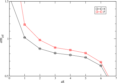
Figure 1: Pi and rho effective masses for $\mu=j=0$.

Range	$m_{\pi}$	$\chi^{2}/N_{df}$	$m_{\rho}$	$\chi^{2}/N_{df}$	$m_{\pi}/m_{\rho}$
3–4	0.809(2)	0.58	0.882(4)	0.71	0.917(3)
3–5	0.800(2)	0.97	0.870(3)	1.4	0.919(3)
3–6	0.795(2)	1.3	0.860(3)	2.5	0.924(3)
4–5	0.789(2)	0.81	0.854(4)	1.7	0.924(3)
4–6	0.786(2)	0.63	0.846(3)	1.9	0.929(3)
5–6	0.783(2)	0.80	0.836(4)	3.0	0.937(3)

Table 2: Fit ranges and fitted masses for pi and rho mesons.

These numbers indicate that we may expect an onset transition at $\mu_{o}\approx m_{\pi}/2\sim 0.4a^{-1}$, but since there is no separation of scales between the Goldstone (pion) and the non-Goldstone (rho), we should not expect chiral perturbation theory to be quantitatively valid at any point.

The static quark potential was computed using APE smeared Wilson loops with spatial separations near the diagonal to minimise lattice artefacts. The minimum time separation used was 2. Figure 2 shows the potential together with a fit to the Cornell potential $V(R)=\sigma R+e/R+C$ up to $aR_{\text{max}}=4.0$. We find for the string tension $\sigma a^{2}=0.218(8)$, which gives $a=0.223(4)$ fm for the lattice spacing.

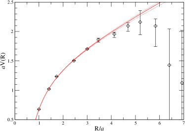
Figure 2: Static quark potential for $\mu=j=0$, together with a fit to the Cornell potential.

4 Results at $\mu\neq 0$

4.1 Model Considerations

Our expectation as $\mu$ is increased from zero at $T\simeq 0$ is that the system will remain in the vacuum phase until an onset occurs at $\mu=\mu_{o}\simeq M_{\text{light}}/N_{c}$, where $M_{\text{light}}$ is the mass of the lightest baryon in the physical spectrum. In QC₂D this lightest baryon is a scalar diquark state in the same chiral multiplet as the pion: hence $\mu_{o}=m_{\pi}/2$, and in the chiral limit the onset transition is well described by an effective chiral model ($\chi$PT) in which only pseudo-Goldstone pion and diquark degrees of freedom are retained. A mean-field treatment of $\chi$PT has yielded quantitative predictions for chiral and superfluid condensates, quark number density, and Goldstone spectrum as $\mu$ is increased beyond onset Kogut:2000ek . Our starting point for thermodynamics is the result for quark number density:

$$n_{\chi PT}=\begin{cases}0\,,&\mu<\mu_{o},\\ 8N_{f}F^{2}\mu\left(1-\frac{\mu_{o}^{4}}{\mu^{4}}\right)\,,&\mu\geq\mu_{o}.\end{cases}$$ (16)

Here $F$ is the pion decay constant, a parameter of the $\chi$PT which can be extracted in principle from the pion correlator measured at $\mu=0$. The pressure follows immediately from integration of the fundamental relation $n_{q}={\partial p/\partial\mu}|_{T,V}$:

$$p_{\chi PT}=4N_{f}F^{2}\left(\mu^{2}+{\frac{\mu_{o}^{4}}{\mu^{2}}}-2\mu_{o}^{2}\right).$$ (17)

Now, if $\Omega(\mu,T,V)$ is the thermodynamic grand potential, then in the grand canonical ensemble $\Omega=-pV$. In the $T=0$ limit we can therefore extract the energy density via $\Omega/V=\varepsilon_{q}-\mu n_{q}$, implying

$$\varepsilon_{\chi PT}=4N_{f}F^{2}\left(\mu^{2}-3\frac{\mu_{o}^{4}}{\mu^{2}}+2\mu_{o}^{2}\right).$$ (18)

We can also extract the trace of the energy-momentum tensor $\delta=\varepsilon_{q}-3p$:

$$\delta_{\chi PT}=8N_{f}F^{2}\left(-\mu^{2}-3\frac{\mu_{o}^{4}}{\mu^{2}}+4\mu_{o}^{2}\right)$$ (19)

and note that $\delta_{\chi PT}$ is positive for $\mu_{o}<\mu<\sqrt{3}\mu_{o}$.

The result (18) for $\varepsilon_{\chi PT}$ coincides with that derived in Kogut:2000ek  using the assumption that diquarks Bose-condense in the ground state, remain degenerate with the pion for $\mu\geq\mu_{o}$, and that their self-interactions are weak due to their Goldstone nature. One infers $\varepsilon_{q}\simeq\frac{1}{2}m_{\pi}n_{q}=\mu_{o}n_{q}$. A more refined treatment taking account of corrections to the dilute ideal Bose gas from the weak repulsive interaction yields Kogut:2000ek

$$\varepsilon_{q}=\mu_{o}n_{q}+{\frac{n_{q}^{2}}{64F^{2}N_{f}}}+\cdots$$ (20)

where the dots denote corrections from subleading terms in the chiral expansion. Using $\mu=\partial\varepsilon_{q}/\partial n_{q}$, this can be seen to be consistent with (16) linearised about $\mu=\mu_{o}$:

$$n_{\chi PT}\approx 32N_{f}F^{2}(\mu-\mu_{o});$$ (21)

the same approximation predicts $p_{\chi PT}$ to vanish as $(\mu-\mu_{o})^{2}$, consistent with a second order transition in the Ehrenfest scheme.

Next we turn to the deconfined phase expected at large $\mu$. The obvious starting point is the Stefan–Boltzmann prediction for the number density of massless quarks:

$$n_{SB}=\frac{N_{f}N_{c}}{3\pi^{2}}\mu^{3}.$$ (22)

This is obtained simply by populating a Fermi sphere of radius $k_{F}=\mu$, with every momentum state occupied by $2N_{f}N_{c}$ non-interacting quarks. Other thermodynamic quantities follow immediately:

$$\varepsilon_{SB}=3p_{SB}={\frac{N_{f}N_{c}}{4\pi^{2}}}\mu^{4};\quad\delta_{SB}=0.$$ (23)

An estimate for the chemical potential $\mu_{d}$ at which deconfinement takes place can be obtained by equating the free grand potential densities, or equivalently the pressures given in (17) and (23). Since $p_{\chi PT}>p_{SB}$ for $\mu<\mu_{d}$ is required for thermodynamic stability, we find $\mu_{d}$ given by the largest positive real root of

$$\mu_{d}^{3}-4\pi F\sqrt{\frac{3}{N_{c}}}(\mu_{d}^{2}-\mu_{o}^{2})=0.$$ (24)

This estimate takes no account of any non-Goldstone states in the hadron spectrum, or of any gluon degrees of freedom released at deconfinement.

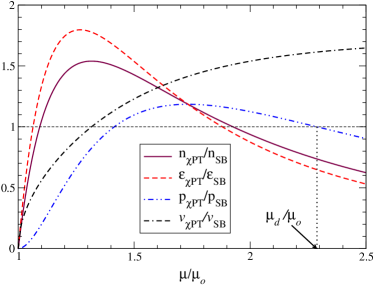
Figure 3: Ratio of thermodynamic observables from $\chi$PT and free quarks

In fig. 3 we plot the ratios $n_{\chi PT}/n_{SB}$, $\varepsilon_{\chi PT}/\varepsilon_{SB}$ and $p_{\chi PT}/p_{SB}$ as functions of $\mu/\mu_{o}$ for the choice $F^{2}=N_{c}/6\pi^{2}$, corresponding to $\mu_{d}\simeq 2.288\mu_{o}$. Since $n_{\chi PT}<n_{SB}$ at this point, this naively simple approach predicts a first order deconfining transition — note also that $\delta_{\chi PT}<0$ at deconfinement. Also shown is the ratio of the speed of sound

$$v_{\chi PT}=\sqrt{\frac{\partial p}{\partial\varepsilon}}=\sqrt{\frac{1-\frac{\mu_{o}^{4}}{\mu^{4}}}{1+3\frac{\mu_{o}^{2}}{\mu^{4}}}}$$ (25)

to the Stefan–Boltzmann value $v_{SB}=1/\sqrt{3}$.

4.2 Thermodynamics results

The raw data for bosonic observables (spatial and temporal plaquettes, Polyakov line) are tabulated in table 3, and for fermionic bilinears ($\langle\bar{\psi}\psi\rangle,n_{q}$ (8), $\varepsilon_{q}$ (9) and $\langle qq\rangle$ (15)) in table 4. All quark observables are normalised to $N_{c}$ colors and $N_{f}$ flavors, with $N_{f}=N_{c}=2$. In this section we outline the analysis needed to extract bulk thermodynamical quantities and condensates.

$j$	$\mu$	$\operatorname{Tr}(\Box_{s}+\Box_{t})/2N_{c}$	$\operatorname{Tr}(\Box_{t}-\Box_{s})/N_{c}$	$\operatorname{Tr}L/N_{c}$
0.00	0.00	0.4738(1)	-0.0002(1)	-0.0014(05)
	0.30	0.4739(3)	0.0001(2)	-0.0008(14)
0.02	0.30	0.4742(3)	0.0002(2)	-0.0012(15)
	0.35	0.4755(4)	-0.0005(3)	0.0005(24)
	0.50	0.4804(5)	0.0024(2)	0.0020(13)
	0.70	0.4773(3)	0.0089(2)	0.0127(11)
0.04	0.25	0.4735(3)	0.0002(3)	-0.0026(14)
	0.30	0.4753(4)	0.0007(4)	-0.0013(20)
	0.35	0.4764(4)	0.0004(2)	0.0003(13)
	0.40	0.4784(4)	0.0012(3)	0.0020(14)
	0.45	0.4792(3)	0.0020(4)	-0.0016(18)
	0.50	0.4799(4)	0.0025(3)	0.0044(15)
	0.55	0.4793(4)	0.0037(3)	0.0004(17)
	0.60	0.4794(3)	0.0051(3)	0.0029(21)
	0.65	0.4778(3)	0.0069(2)	0.0065(11)
	0.70	0.4773(4)	0.0092(3)	0.0094(16)
	0.75	0.4752(2)	0.0122(2)	0.0188(19)
	0.80	0.4719(2)	0.0172(3)	0.0292(12)
	0.90	0.4648(3)	0.0299(3)	0.0719(17)
	1.00	0.4549(3)	0.0442(3)	0.1393(19)
	1.30	0.4277(4)	0.0479(3)	0.4286(20)
	1.40	0.4142(3)	0.0259(4)	0.3216(11)
	1.50	0.4060(2)	0.0128(3)	0.1019(13)
	1.60	0.4052(2)	0.0114(3)	0.0224(18)
	1.75	0.4052(2)	0.0105(4)	0.0018(18)
	2.50	0.4053(3)	0.0115(4)	0.0008(13)
0.06	0.30	0.4767(3)	0.0003(2)	0.0004(16)
	0.50	0.4791(4)	0.0025(2)	-0.0035(14)
	0.70	0.4772(3)	0.0095(4)	0.0094(16)

Table 3: Raw data for gluonic observables

$j$	$\mu$	$n_{q}$	$\varepsilon_{q}$	$\langle\bar{\psi}\psi\rangle$	$\langle qq\rangle$
0.00	0.00	-0.0004(04)	0.3980(4)	14.409(2)	–
	0.30	-0.0008(22)	0.3994(22)	14.399(7)	–
0.02	0.30	0.0012(12)	0.4028(16)	14.389(5)	0.0219(2)
	0.35	0.0030(24)	0.4072(24)	14.364(3)	0.0293(3)
	0.50	0.0382(24)	0.4496(40)	14.254(10)	0.0571(4)
	0.70	0.1506(32)	0.5348(32)	14.178(6)	0.1099(5)
0.04	0.25	0.0036(14)	0.4012(16)	14.396(8)	0.0343(1)
	0.30	0.0102(14)	0.4126(16)	14.360(4)	0.0400(2)
	0.35	0.0144(12)	0.4188(18)	14.332(4)	0.0469(3)
	0.40	0.0252(16)	0.4358(16)	14.292(8)	0.0549(3)
	0.45	0.0332(24)	0.4422(30)	14.272(8)	0.0634(5)
	0.50	0.0476(22)	0.4558(22)	14.244(8)	0.0713(5)
	0.55	0.0648(30)	0.4702(30)	14.236(8)	0.0817(5)
	0.60	0.0898(30)	0.4902(30)	14.196(8)	0.0932(4)
	0.65	0.1238(26)	0.5146(28)	14.180(4)	0.1084(4)
	0.70	0.1660(24)	0.5476(26)	14.156(4)	0.1248(4)
	0.75	0.2302(34)	0.5972(32)	14.136(8)	0.1461(5)
	0.80	0.3354(38)	0.6850(32)	14.084(8)	0.1701(5)
	0.90	0.6664(56)	0.9716(60)	13.916(8)	0.2222(9)
	1.00	1.2602(74)	1.5168(72)	13.560(8)	0.2654(12)
	1.30	5.220(6)	5.284(6)	12.036(8)	0.0956(3)
	1.40	7.040(4)	7.060(4)	11.312(4)	0.0594(1)
	1.50	7.914(4)	7.916(4)	10.944(4)	0.0346(3)
	1.60	7.996(3)	7.996(3)	10.916(4)	0.0255(1)
	1.75	8.000(4)	8.000(4)	10.916(4)	0.0207(1)
	2.50	8.000(2)	8.000(2)	10.924(4)	0.0161(1)
0.06	0.30	0.0130(14)	0.4184(14)	14.331(6)	0.0554(2)
	0.50	0.0530(22)	0.4604(22)	14.230(8)	0.0855(8)
	0.70	0.1780(30)	0.5574(30)	14.131(8)	0.1397(10)

Table 4: Raw data for quark observables (no zero subtraction applied to $\varepsilon_{q}$)

The most straightforward observable to analyse is the quark density $n_{q}$, which as the timelike component of a conserved current requires no renormalisation due to quantum corrections. There may, however, still be lattice artefacts in both UV and IR régimes, as illustrated by the equivalent quantity for free fields on a $N_{s}^{3}\times N_{t}$ lattice:

$$n_{SB}^{\text{lat}}(\mu)=\frac{4N_{f}N_{c}}{N_{s}^{3}N_{t}}\sum_{k}{\frac{i\sin\tilde{k}_{0}\bigl{[}\sum_{i}\cos k_{i}-\frac{1}{2\kappa}\bigr{]}}{\bigl{[}\frac{1}{2\kappa}-\sum_{\nu}\cos\tilde{k}_{\nu}\bigr{]}^{2}+\sum_{\nu}\sin^{2}\tilde{k}_{\nu}}}$$ (26)

where

$$\tilde{k}_{\nu}=\begin{cases}k_{0}-i\mu=\frac{2\pi}{N_{t}}\bigl{(}n_{0}+\frac{1}{2}\bigr{)}-i\mu\,,&\nu=0,\\ k_{\nu}=\frac{2\pi n_{\nu}}{N_{s}}\,,&\nu=1,2,3.\end{cases}$$ (27)

For free massless quarks $\kappa=\frac{1}{8}$. In the large-$\mu$ limit $n_{SB}^{\text{lat}}(\mu)$ saturates at a value $2N_{f}N_{c}$ per lattice site. This is an artefact of non-zero lattice spacing, which we will discuss in more detail in section 4.3 below. For $T=0$ the corresponding continuum relation is (22).

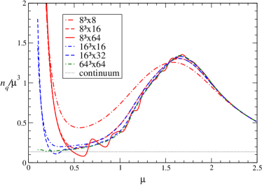
Figure 4: $n_{SB}^{\text{lat}}/\mu^{3}$ for free massless Wilson fermions.

Fig. 4 plots $n_{SB}^{\text{lat}}/\mu^{3}$ for several system sizes, and shows there are significant departures from the continuum result both at small $\mu$ as a result of finite $N_{s}$, and at $\mu a\gtrsim{\cal O}(1)$ as a result of non-zero lattice spacing, species doubling etc. Of particular interest are the pronounced wiggles seen especially on the $8^{3}\times 64$ curve. These arise due to departures from sphericity of the Fermi surface in a finite spatial volume, and are visible whenever the temperature is much smaller than the mode spacing, i.e. $N_{t}\gg N_{s}$ Hands:2002mr .

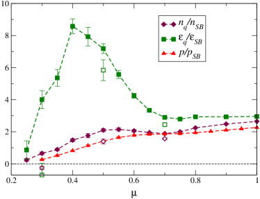
Figure 5: Ratio of thermodynamic observables to free field values versus $\mu$ for $j=0.04$. Open symbols show extrapolations to $j=0$.

The main implication in the window $\mu\in(0.25,1.0)$ where our analysis is focussed is that $n_{SB}^{\text{lat}}$ lies systematically above the continuum value, with the ratio increasing for $\mu>0.5$. To correct for this lattice artefact, we have chosen to plot the ratio $n_{q}/n_{SB}^{\text{lat}}$, shown as a function of $\mu$ in fig. 5. The free field density has been calculated for massless quarks, i.e. with $\kappa=\frac{1}{8}$. In order to assess the systematic error due to our lack of accurate knowledge of the non-zero quark mass, we repeated the free field calculation with $\kappa=0.120$, corresponding to a conservatively large $m_{q}a=0.167$, and found the resulting $n_{SB}^{\text{lat}}(\mu)$ to have a similar shape, with a maximum departure over the $\mu$ range of interest of $O(20\%)$. Where data are available we have plotted as open symbols the result of linearly extrapolating $j\to 0$; at $\mu=0.3$ this yields $n_{q}\approx 0$, consistent with being below the onset expected at $\mu_{o}=m_{\pi}/2$. For $\mu=0.5,0.7$ the extrapolation results in a downwards correction of $O$(20%). We also note that for $\mu\gtrsim 0.5$ the ratio is roughly constant and greater than one, which is plausible if Stefan–Boltzmann scaling sets in at large $\mu$, but with a Fermi momentum $k_{F}>\mu$. Physically, this would result from degenerate quark matter with a positive binding energy arising from interactions. Note that a non-zero quark mass has the opposite effect, tending to raise $\mu$ over $k_{F}$.

In fig. 5, we also plot the unrenormalised quark energy density $\varepsilon_{q}/\varepsilon_{SB}^{\text{lat}}$ versus $\mu$, where $\varepsilon_{SB}^{\text{lat}}$ is evaluated using a formula similar to (26) and $\varepsilon_{SB}^{\text{cont}}$ is given in (23). Note that systematic errors due to non-zero quark mass and incorrect vacuum subtraction are potentially larger in this case, but have maximum impact at the lower end of the $\mu$ range of interest. Once again, a $j\to 0$ extrapolation has been done where possible, and the signal for $\mu=0.3$ is consistent with the vacuum. As for quark number density, the ratio $\varepsilon_{q}/\varepsilon_{SB}^{\text{lat}}$ tends to a constant at large $\mu$, which we interpret as evidence for the formation of a Fermi surface. This limit is approached from above, however, and in the range $0.35\lesssim\mu\lesssim 0.5$ $\varepsilon_{q}/\varepsilon_{SB}$ actually peaks. The implications of this are discussed in section 5.

The pressure $p$ is best calculated using the integral method Engels:1990vr : i.e. $p(\mu)=\int_{\mu_{o}}^{\mu}n_{q}(\mu^{\prime})d\mu^{\prime}$. Note that since the only $\mu$-dependence comes from the quark action, this expression gives in principle the pressure of the entire system including both quarks and gluons. In practice for data taken away from both continuum and thermodynamic limits we should make some attempt to correct for artefacts: we have experimented with two different ad hoc procedures:

$$\text{I}:\quad\frac{p}{p_{SB}}(\mu) =\frac{\int_{\mu_{o}}^{\mu}n_{q}(\mu^{\prime})d\mu^{\prime}}{\int_{\mu_{o}}^{\mu}n_{SB}^{\text{lat}}(\mu^{\prime})d\mu^{\prime}}\,;$$ (28)

$$\text{II}:\quad\frac{p}{p_{SB}}(\mu) =\frac{\int_{\mu_{o}}^{\mu}\frac{n_{SB}^{\text{cont}}}{n_{SB}^{\text{lat}}}(\mu^{\prime})n_{q}(\mu^{\prime})d\mu^{\prime}}{\int_{\mu_{o}}^{\mu}n_{SB}^{\text{cont}}(\mu^{\prime})d\mu^{\prime}}\,,$$ (29)

where $n_{SB}^{\text{cont}}$, $n_{SB}^{\text{lat}}$ are defined in eqs. (22,26) respectively. Ultimately, data from different physical lattice spacings will be required to determine which method is preferred. Using an extended trapezoidal rule to evaluate the integral on the $j=0.04$ data of fig. 5, we have estimated both $p^{I}(\mu)$ and $p^{II}(\mu)$ and plot the results in fig.6.

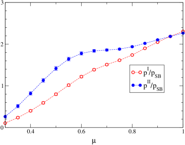
Figure 6: Pressure verus $\mu$ using two different integral methods

In both cases the pressure rises monotonically from near zero at onset, but for method II there is some suggestion of a plateau in $p/p_{SB}$ for $\mu\gtrsim 0.6$. By $\mu\simeq 1.0$ the two methods agree, with $p\approx 2p_{SB}$. This is consistent with the ratio $n_{q}/n_{SB}$ in the same régime, again suggesting a Fermi surface with $k_{F}>\mu$. For comparison with the other fermionic observables we have plotted $p^{II}/p_{SB}$ in fig. 5.

Next we turn to the gluon sector. Since at the current lattice spacing the perturbative correction to the bare gluon energy density is likely to be inadequate, in fig. 7 we content ourselves with plotting unrenormalised data for both $\varepsilon_{g}/\mu^{4}$ and for comparison $\varepsilon_{q}/\mu^{4}$, at $j=0.04$. There is no evidence in our data for any significant variation with $j$ for gluonic observables.

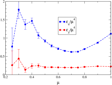
Figure 7: Comparison of bare quark and gluon energy densities versus $\mu$.

The plot illustrates: (i) the significant impact of rescaling the fermionic data by $\varepsilon_{SB}^{\text{lat}}$ (cf. fig. 5); (ii) for all $\mu>\mu_{o}$, the gluonic contribution is a significant fraction of the total energy density; (iii) most strikingly, $\varepsilon_{g}$ scales as $\mu^{4}$ over the whole range of $\mu$. On dimensional grounds, this is the only physically sensible possibility if thermal effects are negligible. We reiterate that gluonic contributions to thermodynamic observables are not present in the SB formulae (23), so that observations (ii) and (iii) are non-trivial predictions of the simulation. Note that our lack of knowledge about the energy density renormalisation factors prevents us from making any quantitative estimate of the gluon energy density as proportion of the total energy density.

The quark and gluon contributions to the conformal anomaly (14,13) are plotted in fig. 8.

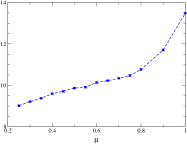
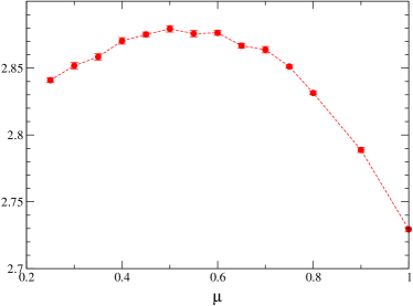
Figure 8: Top: $\kappa^{-1}\operatorname{Tr}(1\kern-4.5pt1-\langle\bar{\psi}\psi\rangle)$, and bottom: $3\beta/N_{c}\operatorname{Tr}\langle\Box_{t}+\Box_{s}\rangle$, as functions of $\mu$ at $j=0.04$.

As for energy density, the raw data requires a zero-$\mu$ subtraction. To extract $\delta$, we also need information on the lattice beta-functions, which require an extensive simulation campaign and are not yet available. For this reason we restrict ourselves to qualitative remarks. The quark contribution shown in the upper panel of fig. 8 increases monotonically from $\mu=0$. The sign of $\partial\kappa/\partial a$ is found to be negative in QCD simulations AliKhan:2001ek ; Gockeler:2004rp (although it can change sign as the chiral limit $\kappa\to\kappa_{c}$ is approached away from the continuum limit AliKhan:2001ek ). This is in accord with what we have found in our SU(2) simulations at various $\beta,\kappa$ Skullerud:2003yc . We conclude that the quark contribution to $\delta$ is negative. The gluon contribution, by contrast, starts positive for $\mu_{o}\lesssim\mu\lesssim 0.6$ before changing sign to decrease montonically for $\mu>0.6$ (recall $\partial\beta/\partial a<0$ due to asymptotic freedom).

In fact, we expect the gluon contribution to dominate, since $\delta\kappa/\delta\beta\approx{\cal O}(0.01)$ along lines of constant physics Gockeler:2004rp . This is clearly required for consistency with fig. 5, since the sign of $\delta$ must coincide with the sign of $\varepsilon/\varepsilon_{SB}-p/p_{SB}$, which looks positive for $0.4\lesssim\mu\lesssim 0.6$. We also get a clue about the unknown renormalisation factor for $\varepsilon_{q}$, since if $\delta$ is to go negative at large $\mu$, $\varepsilon_{\text{ren}}/\varepsilon_{SB}<p/p_{SB}$ in this régime.

The non-monotonic behaviour of the plaquette has been predicted in a $\chi$PT study in which asymptotic freedom of the gauge coupling is taken into account Metlitski:2005db , and has also been observed in recent simulations with staggered fermions Alles:2006ea . It can be understood in terms of Pauli blocking. In quark matter as $\mu$ increases, the number of $q\bar{q}$ pairs available for vacuum polarisation corrections to the gluon decreases, since only states close to the Fermi surface can participate. In the limit of complete saturation (i.e. one quark of each color, flavor and spin per lattice site) the gluon dynamics hence resembles that of the quenched theory, so $\operatorname{Tr}\Box(\mu\to\infty)<\operatorname{Tr}\Box(\mu=0)$. Assuming a smooth passage to the limit we deduce $\delta<0$ at large $\mu$.

To summarise the thermodynamic information, we have been able to extract $n_{q}(\mu)$ and $p(\mu)$ directly from the simulation — any remaining UV and IR artefacts in fig. 5 can be controlled by simulations closer to thermodynamic and continuum limits. The status of $\varepsilon_{q},\varepsilon_{g}$ is less secure, because these quantities require renormalisation by an as yet undetermined factor; similarly the trace of the energy-momentum tensor $\delta$ requires knowledge of the lattice beta-functions. In each case, though, the rescaling factor is $\mu$-independent, so the shape of the data in figs. 5 and 8 is correct. However, the behaviour of $\varepsilon_{q}$ in fig. 5, and $\delta_{g}$ in fig. 8 give a strong hint of two qualitatively distinct high density regions: (i) for $\mu_{o}\lesssim\mu\lesssim 0.65$ $\varepsilon_{q}\approx O(5\varepsilon_{SB})$, and $\delta_{g}>0$; (ii) for $\mu\gtrsim 0.65$ $\varepsilon_{q}/\varepsilon_{SB}\approx n_{q}/n_{SB}$, $\delta_{g}<0$. All thermodynamic quantities seem to have the same $\mu$-scaling as their Stefan–Boltzmann counterparts in this higher density régime, although $n_{q}/n_{SB}\approx p/p_{SB}\approx 2$.

4.3 The approach to saturation

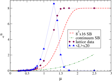
Figure 9: Quark number density $n_{q}$ and Polyakov loop $L$ vs. $\mu$ for values up to $\mu=2.5$. All lattice data are at $j=0.04$.

In figure 9 we plot $n_{q}(\mu)$ including values of $\mu$ up to 2.5, as tabulated in tables 1, 3 and 4, together with both continuum (22) and lattice (26) expectations for non-interacting quarks. On any system with a non-zero lattice spacing, there is a point at which every lattice site is occupied by the maximum value $2N_{c}N_{f}$ allowed by the Pauli exclusion principle. For free Wilson fermions this occurs for $\mu a\approx 2.0$; for the interacting quarks studied here the saturation threshold drops to $\mu a\approx 1.5$. We also see that the relation $n_{q}\approx 2n_{SB}^{\rm lat}$ continues to hold all the way up to the threshold; there is no sign of asymptotic freedom. In this respect, the situation bears some similarity to that of QCD at temperatures between $T_{c}$ and $3T_{c}$, where lattice simulations have also uncovered a deconfined, but still strongly interacting system. The nature of this system is quite different, however, as in the high-temperature case a slow approach towards Stefan–Boltzmann predictions is observed, while in the present case the strong binding energy remains unchanged in the entire domain studied.

As discussed above, in a saturated system, virtual $q\bar{q}$ pairs are suppressed, leading to the expectation that the gluodynamics should be that of the quenched theory. In fact, inspection of table 3 shows this is a little simplistic, since $\varepsilon_{g}$ remains non-vanishing even once saturation is complete. Strong coupling considerations suggest that the saturated system has a quark-induced effective action that can be expanded in even powers of the Polyakov loops. The resulting $S_{\text{eff}}$ distinguishes between $\Box_{s}$ and $\Box_{t}$ hence yielding $\varepsilon_{g}\not=0$, but respects the global $Z_{2}$ centre symmetry of the quenched action, consistent with $\langle\operatorname{Tr}L\rangle=0$.

Just below saturation, $\operatorname{Tr}L$ rises rapidly. In this régime the theory resembles a p-type semiconductor, in that the low energy excitations are de-confined holes. The holes appear weakly interacting: $\langle qq\rangle$, which also measures the density of hole-hole pairs, is small, and there is little evidence from $N_{cg}$ (table 1) for a light bound state.

4.4 Order parameters

Might it be possible to reconcile the behaviour reported in section 4.2 with the models of section 4.1? To elucidate this question we next review order parameters for superfluidity and deconfinement.

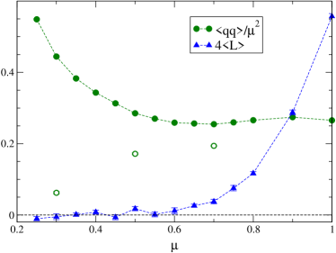
Figure 10: The Polyakov loop $L$ and the superfluid diquark condensate $\langle qq\rangle/\mu^{2}$ for $j=0.04$ as function of $\mu$. Open symbols show $\langle qq\rangle/\mu^{2}$ extrapolated to $j=0$.

In fig. 10 we plot both the superfluid condensate $\langle qq\rangle$ given in (15), rescaled by a factor $\mu^{-2}$, and the Polyakov loop $L$. Both show a marked change of behaviour at $\mu\simeq 0.6$; for $\mu$ greater than this value $\langle qq\rangle/\mu^{2}$ is approximately constant, while $L$ rises from zero. To interpret the superfluid condensate, we first need to compare data taken at varying $j$, shown in fig. 11 together with a linear extrapolation to $j=0$.

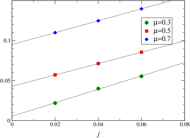
Figure 11: Superfluid condensate $\langle qq\rangle$ vs. $j$ for various $\mu$

The slight non-linearity of the $\mu=0.3$ data suggests that below onset, $\lim_{j\to 0}\langle qq\rangle=0$, whereas for $\mu=0.5$, 0.7 the data extrapolate to a non-vanishing intercept, implying a non-vanishing condensate and hence spontaneous breaking of baryon number symmetry, i.e. superfluidity. Extrapolated values are plotted as open symbols in fig. 10.

Now, in the Bose condensate phase expected for $\mu_{o}<\mu<\mu_{d}$, $\chi$PT predicts Kogut:2000ek

$$\frac{\langle qq\rangle_{\chi PT}}{\mu^{2}}\propto\frac{1}{\mu^{2}}\sqrt{1-\frac{\mu_{o}^{4}}{\mu^{4}}},$$ (30)

which is a monotonically decreasing function for $\mu\geq\root 4 \of{2}\mu_{o}$. For a Fermi surface perturbed by a weak $qq$ attractive force, by contrast, the order parameter counts the number of Cooper pairs condensed in the ground state, which all originate in a shell of thickness $\Delta$ around the Fermi surface, where $\Delta$ is the superfluid gap: hence

$$\frac{\langle qq\rangle_{BCS}}{\mu^{2}}\propto\Delta.$$ (31)

The data of fig. 10 support this scenario for $\mu\gtrsim 0.6$, with $\Delta$ independent of $\mu$. Further support for the importance of quark degrees of freedom at large $\mu$ comes from the Polyakov loop, which rises smoothly from zero at $\mu\simeq 0.65$. We thus tentatively assign $\mu_{d}\simeq 0.65$, marking a transition from confined scalar “nuclear” matter to deconfined quark matter. In condensed matter physics parlance this transition would be characterised as one from BEC to BCS. Exposing the detailed nature of the transition will require many more simulations using a variety of source strengths, lattice spacings, and spatial volumes.

4.5 Static quark potential

The screening effect of the dense medium can be further investigated by studying how the static quark potential changes as the chemical potential increases. In figure 12 we show the static quark potential for various values of $\mu$ and $j=0.04$. Up to $\mu=0.3$ there is no change from the $\mu=0$ potential, while in the intermediate phase we see clear evidence of screening due to a nonzero baryon density. This is even clearer in fig. 13, where the $\mu=j=0$ potential has been factored out.

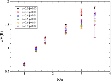
Figure 12: The static quark potential for various values of the chemical potential $\mu$ and diquark source $j=0.04$, together with the $\mu=j=0$ potential shown in fig. 2.

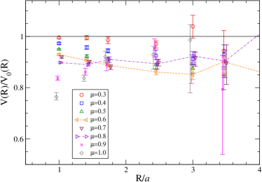
Figure 13: The static quark potential for various values of the chemical potential $\mu$ and diquark source $j=0.04$, divided the $\mu=j=0$ potential shown in fig. 2.

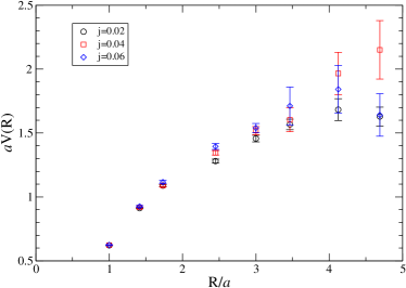
Figure 14: The static quark potential at $\mu=0.7$ for different values of $j$.

In the deconfined phase a new pattern emerges, where the short distance potential is strongly modified, while at long distances we appear to see an increase with increasing $\mu$ rather than a decrease as expected. There are however indications that the long-distance screening at $\mu=0.7$ may become slightly stronger as $j\to 0$, as fig. 14 shows. No dependence on $j$ is seen at $\mu=0.3$ or $\mu=0.5$. We do not have an understanding of these effects at present, although it is possible that lattice artefacts may contribute to the short-distance modifications. This can be resolved by going to finer lattices. Likewise, larger lattices will be required to determine the long distance potential to greater accuracy.

4.6 Gluon propagator

We have computed the gluon propagator by fixing the configurations to Landau gauge using an overrelaxation algorithm to a precision $|\partial_{\nu}A_{\nu}|^{2}<10^{-10}$. The approach and notation is analogous to that of Leinweber:1998uu . At nonzero chemical potential, which defines a preferred rest frame, the gluon propagator can be decomposed as

$$\begin{split}D_{\mu\nu}(q)&=P^{M}_{\mu\nu}(q)D_{M}(q_{0}^{2},\vec{q}^{2})\\ &\phantom{=}+P^{E}_{\mu\nu}(q)D_{E}(q_{0}^{2},\vec{q}^{2})+P^{L}_{\mu\nu}(q)D_{L}(q_{0}^{2},\vec{q}^{2})\,,\end{split}$$ (32)

where

$$P^{M}_{ij}(q) =(\delta_{ij}-\frac{q_{i}q_{j}}{\vec{q}^{2}})\,;\quad P^{M}_{00}(q)=P^{M}_{i0}=0\,;$$ (33)

$$P^{E}_{\mu\nu}(q) =\delta_{\mu\nu}-\frac{q_{\mu}q_{\nu}}{q_{0}^{2}+\vec{q}^{2}}-P^{M}_{\mu\nu}(q)\,;$$ (34)

$$P^{L}_{\mu\nu}(q) =\frac{q_{\mu}q_{\nu}}{q_{0}^{2}+\vec{q}^{2}}\,;$$ (35)

$$q_{\nu} =\frac{2}{a}\sin\Bigl{(}\frac{\pi n_{\nu}}{L_{\nu}}\Bigr{)},\quad n_{\nu}=-\frac{L_{\nu}}{2}+1,\ldots,\frac{L_{\nu}}{2}\,.$$ (36)

$D_{M}$ is the magnetic (spatially transverse) gluon propagator and $D_{E}$ is the electric (spatially longitudinal) propagator, while the longitudinal propagator $D_{L}$ is zero in Landau gauge.

Figure 15 shows the gluon propagator at $\mu=j=0$ as a function of 4-momentum $q^{2}=q_{0}^{2}+\vec{q}^{2}$. Since the Lorentz symmetry remains unbroken here there is only one form factor, and the small splitting between electric and magnetic gluon is most likely a finite volume effect, similar to the asymmetric finite volume effects on the tensor structure observed in the SU(3) gluon propagator Leinweber:1998uu .

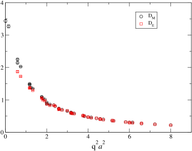
Figure 15: Gluon propagator at $\mu=j=0$.

Figure 16 shows the gluon propagator at $\mu=0.7,j=0.04$ as function of the 4-momentum $q^{2}$, compared to the vacuum gluon propagator. We find that the electric propagator remains virtually unchanged at this point, while some modifications can be seen in the magnetic propagator. In particular, the Lorentz or O(4) symmetry is clearly broken since different values for $q_{0}$ give different “branches”.

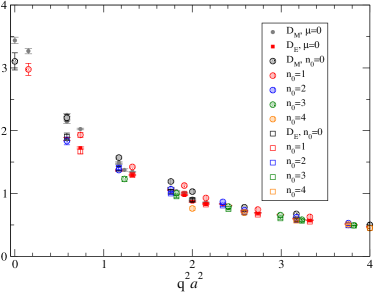
Figure 16: Gluon propagator at $\mu=0.7,j=0.04$, together with the $\mu=j=0$ propagator for comparison.

In order to see the $\mu$-evolution more clearly, we show in fig. 17 the magnetic gluon propagator for the lowest two Matsubara modes $n_{0}=0,1$ as function of the spatial momentum $|\vec{q}|$ for different $\mu$. We see that there is very little change up to the deconfinement transition, after which there is a dramatic infrared suppression and clear ultraviolet enhancement of the propagator. These changes makes it look more like an ordinary massive boson propagator, i.e., the gluon has acquired a magnetic mass which grows as $\mu$ increases beyond $\mu_{d}$. This effect does depend on the diquark source $j$, becoming weaker as $j\to 0$, as figure 19 shows. Simulations at smaller $j$ in the deconfined phase will be necessary to firm up the picture, but it seems unlikely that the $j$ dependence seen at $\mu=0.7$ will be sufficient to wholly cancel the infrared screening effect. No dependence on $j$ is seen at $\mu=0.3,0.5$.

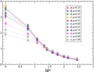
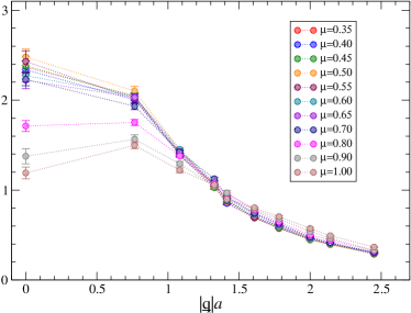
Figure 17: Magnetic gluon propagator for $q_{0}=0$ (top) and $aq_{0}=2\sin\pi/16$ (bottom) and diquark source $j=0.04$, as a function of spatial momentum $|\vec{q}|$ for various values of the chemical potential.

Figure 18 shows the electric propagator for the lowest two Matsubara modes, for selected values of $\mu$. While the electric propagator, as seen previously, remains unchanged up to $\mu=0.7$, it too is clearly suppressed in the infrared above deconfinement (although to a smaller extent than the magnetic case), but appears unchanged in the ultraviolet. No dependence on the diquark source is seen. The same effects can be seen in both static ($q_{0}=0$) and non-static propagators, although for $n_{0}\geq 2$ the splitting between electric and magnetic sectors becomes harder to detect. The case of the static magnetic propagator is particularly interesting, since this is unscreened to all orders in perturbation theory, yet we observe a clear screening effect. The increase of magnetic screening with $j$ also suggests a non-perturbative origin, hinting at a relation to the non-vanishing $\langle qq\rangle$ condensate, rather than the presence of light quasiquark degrees of freedom at the Fermi surface. The data in this case may be distorted by possible finite volume effects, although the consistency between the $n_{0}=0$ and $n_{0}=1$ data indicates that these do not affect the qualitative picture.

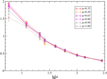
Figure 18: As fig. 17, for the electric gluon propagator.

Figure 19: Magnetic gluon propagator at $\mu=0.7$ for various values of the diquark source $j$.

5 Discussion and outlook

Our results indicate that, at least for the (rather heavy) quark mass employed in this study, QC₂D has three separate phases:

1. A vacuum phase, for $\mu<\mu_{o}\approx m_{\pi}/2$, where the baryon density remains zero and all other physical quantities (with the likely exception of the hadron spectrum Kogut:2000ek ) are unchanged.

2. A confined, bosonic superfluid phase, for $\mu_{o}<\mu<\mu_{d}$, characterised by Bose–Einstein condensation of scalar diquarks. The thermodynamics of this phase can be qualitatively (but not quantitatively) described by chiral perturbation theory, and the static quark potential is screened by the dense medium.

3. A deconfined phase, for $\mu>\mu_{d}$, where quarks and gluons are the dominant degrees of freedom. In this phase, a Fermi surface of quarks is built up, leading to scaling of thermodynamic quantities of the same form as predicted by the Stefan–Boltzmann form, but with a different constant of proportionality. We interpret the latter as evidence for a non-zero binding energy in this phase, as $k_{F}>E_{F}$. We observe Debye screening of the electric gluon propagator, as well as strong screening of both static and non-static magnetic gluon modes.

The deconfinement transition occurs at $a\mu_{d}\approx 0.65$, which in physical units corresponds to $\mu_{d}\approx 600$ MeV. The corresponding quark density may be estimated as $n_{q}\approx 11\mbox{fm}^{-3}$ directly from table 4, or from fig. 5 where lattice artefacts are taken into account, as $\approx$6.5fm^-3.

Let us discuss some phenomenological implications of our results. First consider the nature of the deconfinement transition. Since both the low density “nuclear matter” and high density “quark matter” phases are characterised by a U(1)_B breaking superfluid condensate, it is tempting to postulate the quark/hadron continuity proposed for QCD with $N_{f}=3$ light flavors in Schafer:1998ef . In that case, the spectrum of physical excitations in both nuclear and quark phases is qualitatively similar and can be matched using phenomenological insight, for instance that the physical state with the smallest energy per baryon is the 6-quark bosonic state known as the H-dibaryon, which can Bose-condense to form a superfluid at nuclear densities. In QC₂D, however, no matching is possible. The spectrum in the confined phase consists entirely of bosonic states, be they $q\bar{q}$ mesons, $qq$ baryons and their conjugates, or glueballs. The deconfined phase by contrast has quasiquark excitations with half-integer spin and mass gap $\Delta$, the same energy scale as all non-Goldstone mesonic and baryonic excitations. The only states which are conceivably lighter are spin-1 quasigluons, with no counterpart in the low-energy spectrum predicted by $\chi$PT Kogut:2000ek . Since the spectrum is discontinuous, it seems natural to suggest that deconfinement in this case is a genuine phase transition, rather than a crossover.

The most intriguing of our results concern the magnetic gluon propagator shown in fig. 17. The long-distance screening observed in the static limit $q_{0}\to 0$ is not predicted at any order of perturbation theory. However, this breakdown of perturbation theory should not be unexpected as the magnetic gluon is an intrinsically non-perturbative object. We have no explanation for the screening effect, but note that absence of magnetic screening in the static limit is a crucial ingredient of the celebrated calculation of the gap scaling $\Delta\propto\exp(-3\pi^{2}/\sqrt{2}g)$ predicted for high-density QCD Son:1998uk .

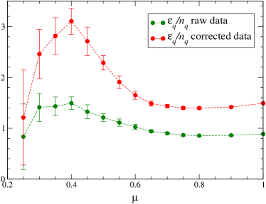
Figure 20: The ratio $\varepsilon_{q}/n_{q}$ vs. $\mu$, using both the raw data of table 4, and rescaled by a factor $n_{SB}^{\text{lat}}/\varepsilon_{SB}^{\text{lat}}$

Finally, it is fascinating to speculate on the astrophysical consquences of our results. Figure 20 plots the energy per quark $\varepsilon_{q}/n_{q}$ against $\mu$, and shows a shallow minimum at $\mu a\approx 0.8$. This feature occurs whether or not corrections for lattice artefacts are applied, and appears to be a robust prediction of our simulation. Inclusion of the gluon contribution $\varepsilon_{g}$ shown in fig. 7 will ensure $\partial\varepsilon/\partial n_{q}>0$ as $\mu\to\infty$, as of course will recovery of the Stefan–Boltzmann scaling (22,23) as asymptotic freedom sets in. Moreover, the minimum is not predicted by $\chi$PT, where $\varepsilon$ increases monotonically with $n_{q}$ (see eq.(20)). The minimum resembles a property known as saturation in nuclear physics, and implies that objects formed from a fixed number of baryons, such as stars, will assume their ground states when the majority of the material lies in its vicinity. Since the minimum lies above the deconfining transition, we deduce that two-color stars are made of quark matter.

Orthodox models of quark stars Glendenning:2000 are based on a simple equation of state such as the Bag Model, which predicts a sharp first order deconfining transition. The resulting stars have a sharp surface where $p=0$, along which quark matter coexists with the vacuum. In QC₂D by contrast, the state of minimum $\varepsilon/n_{q}$ has $p>0$. A two-color star must therefore have a thin surface layer, perhaps better described as an atmosphere, formed from scalar diquark baryons, and whose density falls continuously to zero as the surface is approached. Matter in the range $0.4\lesssim\mu a\lesssim 0.7$, is mechanically unstable, since according to fig. 5 $\partial p/\partial\varepsilon<0$ and the resulting sound speed imaginary. At the base of the diquark atmosphere there will be a sharp increase in both pressure and density, and the bulk of the star will be formed from quark matter with $\mu>\mu_{d}$. Precise radial profiles, and the relation between the star mass $M$ and its radius $R$, must await more quantitative information of the equation of state, which requires the correct normalisation of $\varepsilon_{q}$ and $\varepsilon_{g}$.

We finish by outlining future directions of study. The lattice spacing used here is quite coarse, and as illustrated in section 4.2 lattice artefacts are quite substantial. It will be important to repeat the study on finer lattices in order to gain control over these artefacts. This is currently underway.

It will also be desirable to find the correct rescaling factors for the energy densities, via a non-perturbative determination of the Karsch coefficients using simulations on anisotropic lattices Levkova:2006gn ; Morrin:2006tf .

Since the differences between QCD and QC₂D are greatest in the chiral limit, the heavy quark mass employed here can be considered a positive rather than a negative. Nonetheless, it would be desirable to study a system with lighter quarks, to explore the mass dependence of our results and interpolate between the régime we have been exploring and the chiral régime. Better control over the limit $j\to 0$ is also required.

Beyond the issues considered in this paper, we are intending to study the hadron (meson and diquark) spectrum and the fate of Goldstone as well as non-Goldstone modes in the dense medium. Issues of interest there are the fate of the vector meson and the possibility that it becomes light in the dense phase Brown:1991kk ; Sannino:2001fd ; Muroya:2002ry . Also of interest is the pseudoscalar diquark, which may provide a pointer to the restoration of the U(1)_A symmetry in the medium Schafer:2002yy . We also intend to study the Gor’kov quark propagator in momentum space, which will provide information about effective quark masses and the superfluid diquark gap. Gauge-invariant approaches to identifying the presence of a Fermi surface in a Euclidean simulation can also be employed Hands:2003dh . Finally, once ensembles of the dense medium are available on a fine lattice, it will be interesting to analyse topological excitations Alles:2006ea , to see to what extent deconfinement in dense baryonic matter resembles deconfinement in a hot medium.

References

- (1) K. Rajagopal and F. Wilczek, The condensed matter physics of QCD, in At the Frontier of Particle Physics: Handbook of QCD, edited by M. Shifman, p. 2061, Singapore, 2001, World Scientific, [hep-ph/0011333].
- (2) M. G. Alford, Ann. Rev. Nucl. Part. Sci. 51, 131 (2001), [hep-ph/0102047].
- (3) T. Schäfer, hep-ph/0304281, Lectures given at 14th National Nuclear Physics Summer School, Santa Fe, New Mexico, 28 Jul - 10 Aug 2002.
- (4) I. A. Shovkovy, Found. Phys. 35, 1309 (2005), [nucl-th/0410091].
- (5) O. Philipsen, PoS LAT2005, 016 (2005), [hep-lat/0510077].
- (6) S. Hands, J. B. Kogut, M.-P. Lombardo and S. E. Morrison, Nucl. Phys. B558, 327 (1999), [hep-lat/9902034].
- (7) R. Aloisio, V. Azcoiti, G. Di Carlo, A. Galante and A. F. Grillo, Phys. Lett. B493, 189 (2000), [hep-lat/0009034].
- (8) S. Hands et al., Eur. Phys. J. C17, 285 (2000), [hep-lat/0006018].
- (9) S. Hands, I. Montvay, L. Scorzato and J. Skullerud, Eur. Phys. J. C22, 451 (2001), [hep-lat/0109029].
- (10) J. B. Kogut, D. Toublan and D. K. Sinclair, Nucl. Phys. B642, 181 (2002), [hep-lat/0205019].
- (11) S. Muroya, A. Nakamura and C. Nonaka, Phys. Lett. B551, 305 (2003), [hep-lat/0211010].
- (12) B. Allés, M. D’Elia and M. P. Lombardo, hep-lat/0602022.
- (13) S. Chandrasekharan and F.-J. Jiang, hep-lat/0602031.
- (14) L. A. Kondratyuk, M. M. Giannini and M. I. Krivoruchenko, Phys. Lett. B269, 139 (1991).
- (15) S. Dürr, PoS LAT2005, 021 (2005), [hep-lat/0509026].
- (16) M. Golterman, Y. Shamir and B. Svetitsky, hep-lat/0602026.
- (17) W. Bietenholz and U. J. Wiese, Phys. Lett. B426, 114 (1998), [hep-lat/9801022].
- (18) J.-I. Skullerud, S. Ejiri, S. Hands and L. Scorzato, hep-lat/0312002.
- (19) J. B. Kogut, D. K. Sinclair, S. J. Hands and S. E. Morrison, Phys. Rev. D64, 094505 (2001), [hep-lat/0105026].
- (20) F. Karsch and I. O. Stamatescu, Phys. Lett. B227, 153 (1989).
- (21) F. Karsch, Nucl. Phys. B205, 285 (1982).
- (22) C. R. Allton et al., Phys. Rev. D68, 014507 (2003), [hep-lat/0305007].
- (23) J. Kogut, M. Stephanov, D. Toublan, J. Verbaarschot and A. Zhitnitsky, Nucl. Phys. B582, 477 (2000), [hep-ph/0001171].
- (24) S. Hands and D. N. Walters, Phys. Lett. B548, 196 (2002), [hep-lat/0209140].
- (25) J. Engels, J. Fingberg, F. Karsch, D. Miller and M. Weber, Phys. Lett. B252, 625 (1990).
- (26) CP-PACS, A. Ali Khan et al., Phys. Rev. D64, 074510 (2001), [hep-lat/0103028].
- (27) QCDSF–UKQCD, M. Göckeler et al., hep-ph/0409312.
- (28) M. A. Metlitski and A. R. Zhitnitsky, Nucl. Phys. B731, 309 (2005), [hep-ph/0508004].
- (29) UKQCD, D. B. Leinweber, J. I. Skullerud, A. G. Williams and C. Parrinello, Phys. Rev. D60, 094507 (1999), [hep-lat/9811027].
- (30) T. Schäfer and F. Wilczek, Phys. Rev. Lett. 82, 3956 (1999), [hep-ph/9811473].
- (31) D. T. Son, Phys. Rev. D59, 094019 (1999), [hep-ph/9812287].
- (32) N. K. Glendenning, Compact Stars (Springer-Verlag, New York, 2000).
- (33) L. Levkova, T. Manke and R. Mawhinney, Phys. Rev. D73, 074504 (2006), [hep-lat/0603031].
- (34) R. Morrin, A. Ó Cais, M. Peardon, S. M. Ryan and J.-I. Skullerud, hep-lat/0604021.
- (35) G. E. Brown and M. Rho, Phys. Rev. Lett. 66, 2720 (1991).
- (36) F. Sannino and W. Schäfer, Phys. Lett. B527, 142 (2002), [hep-ph/0111098].
- (37) T. Schäfer, Phys. Rev. D67, 074502 (2003), [hep-lat/0211035].
- (38) S. Hands, J. B. Kogut, C. G. Strouthos and T. N. Tran, Phys. Rev. D68, 016005 (2003), [hep-lat/0302021].