Two-flavor QCD Thermodynamics using Anisotropic Lattices

Abstract

Numerical simulations of full QCD on anisotropic lattices provide a convenient way to study QCD thermodynamics with fixed physics scales and reduced lattice spacing errors. We report results from calculations with two flavors of dynamical staggered fermions, where all bare parameters and the renormalized anisotropy are kept constant and the temperature is changed in small steps by varying only the number of time slices. Including results from zero-temperature scale setting simulations, which determine the Karsch coefficients, allows for the calculation of the equation of state at finite temperatures.

I Introduction

Lattice calculations provide a method to study the properties of the quark-gluon plasma (QGP), which is considered to be the phase matter existed in at the extreme range of temperatures microseconds after the big bang. To understand the basic character of the QGP we need to determine the equation of state (EOS) for the system in a regime of strong gauge coupling for which a non-perturbative scheme for calculation is most adequate. Currently in the lattice formulation of QCD two different approaches to that problem could be adopted. One of them is the derivative (operator) method which requires the knowledge of the asymmetry coefficients, or Karsch coefficients [1, 2]. These coefficients have been evaluated only perturbatively [3, 4] since their non-perturbative values are not trivial to calculate in practice [5]. The second method is the integral method [6, 7], which does not require the values of the Karsch coefficients, but has the disadvantage that for a given quark mass at a single temperature a number of different simulations are required, and in addition, there exist the problems of scaling violation. In our study we avoid these disadvantages by choosing the derivative method implemented for anisotropic lattices in combination with a fixed parameter scheme described below.

The anisotropic formulation of lattice QCD has certain advantages regarding the study of the equation of state at various finite temperatures. Finite temperature field theory has a natural asymmetry which makes the anisotropic approach useful to reduce the lattice spacing errors associated with the transfer matrix at less cost than is required for the full continuum limit [8]. Through the introduction of anisotropy on the lattice one can make the temporal lattice spacing, $a_{t}$, sufficiently small so that by varying the number of time slices, $N_{t}$, the temperature can be changed in small discrete steps.

To study the thermodynamic properties of the quark-gluon system we simulate QCD with two flavors of dynamical staggered fermions on anisotropic lattice. The fixed parameter scheme we employ to avoid scaling violations is the following. All the bare parameters of the simulation are kept constant and only the temperature is changed by varying $N_{t}$ (from 4 to 64). This approach separates temperature and lattice spacing effects and keeps the underlying physics scales (i.e. the lattice spacings in temporal and spatial directions, respectively $a_{t}$ and $a_{s}$) fixed.

The calculation of EOS of the quark-gluon system involves derivatives of the bare parameters with respect to the physical anisotropy $\xi=a_{s}/a_{t}$ and the spatial lattice spacing $a_{s}$. These are the already mentioned above Karsch coefficients, which can be obtained non-perturbatively as a by-product of the zero-temperature calculations needed to choose the bare parameters. In our scheme, once calculated, the Karsch coefficients can be used for all temperatures since they depend only on the intrinsic lattice parameters and not on $N_{t}$. This allows a straightforward determination of the temperature dependence of the energy and pressure, again at fixed lattice spacing. With two or more slightly different values for $a_{t}$, a high-resolution sampling of temperatures can be investigated.

This paper is organized as follows. In section II, we define the anisotropic staggered action and derive analytic expressions for the energy and pressure for the studied system. In section III we describe the scale-setting techniques. Section IV investigates the phase transition for the staggered fermions as we change the temperature in small steps. In section V we present the technique used to calculate the Karsch coefficients and the numerical results for them. Section VI contains the numerical results for the EOS for two anisotropies, $\xi=4.0(1)$ and $\xi=4.8(3)$. In Section VII we examine our data for evidence for improvement of the flavor symmetry, when due to the anisotropy $a_{t}$ becomes sufficiently small. Our conclusions are given in section VIII.

II Action and General Analytic Framework

In this section we define the action we use and derive the analytical form of the EOS using the derivative method.

We work with an asymmetric lattice in Euclidean space with notation for the spatial lattice spacing $a_{s}$ and temporal lattice spacing $a_{t}$. Our calculations are based on the QCD action $S=S_{G}+S_{F}$, where the gauge part is the standard anisotropic Wilson action [9]:

$$S_{G} = -\frac{\beta}{N_{c}}\left[\frac{1}{\xi_{o}}\sum_{x,s>s^{\prime}}{\rm Re}{\rm Tr}\left[P_{ss^{\prime}}(x)\right]+\xi_{o}\sum_{x,s}{\rm Re}{\rm Tr}\left[P_{st}(x)\right]\right]$$ (1)

and the fermion part is the standard staggered action [10] with anisotropy introduced in the spirit of [9] :

$$S_{F} = \sum_{x}\overline{\psi}(x)\left[m_{f}+\nu_{t}\mathchoice{\ooalign{$\hfil\displaystyle\mkern 1.0mu/\hfil$\crcr$\displaystyle D$}}{\ooalign{$\hfil\textstyle\mkern 1.0mu/\hfil$\crcr$\textstyle D$}}{\ooalign{$\hfil\scriptstyle\mkern 1.0mu/\hfil$\crcr$\scriptstyle D$}}{\ooalign{$\hfil\scriptscriptstyle\mkern 1.0mu/\hfil$\crcr$\scriptscriptstyle D$}}_{t}+\frac{\nu_{s}}{\xi_{o}}\sum_{s}\mathchoice{\ooalign{$\hfil\displaystyle\mkern 1.0mu/\hfil$\crcr$\displaystyle D$}}{\ooalign{$\hfil\textstyle\mkern 1.0mu/\hfil$\crcr$\textstyle D$}}{\ooalign{$\hfil\scriptstyle\mkern 1.0mu/\hfil$\crcr$\scriptstyle D$}}{\ooalign{$\hfil\scriptscriptstyle\mkern 1.0mu/\hfil$\crcr$\scriptscriptstyle D$}}_{s}\right]\psi(x).$$ (18)

In the above definitions $P_{ss^{\prime}}$ and $P_{st}$ are the space-space and space-time plaquette variables. The bare anisotropy parameter $\xi_{o}=\xi$ at the tree level. $\mathchoice{\ooalign{$\hfil\displaystyle\mkern 1.0mu/\hfil$\crcr$\displaystyle D$}}{\ooalign{$\hfil\textstyle\mkern 1.0mu/\hfil$\crcr$\textstyle D$}}{\ooalign{$\hfil\scriptstyle\mkern 1.0mu/\hfil$\crcr$\scriptstyle D$}}{\ooalign{$\hfil\scriptscriptstyle\mkern 1.0mu/\hfil$\crcr$\scriptscriptstyle D$}}_{t}$ and $\mathchoice{\ooalign{$\hfil\displaystyle\mkern 1.0mu/\hfil$\crcr$\displaystyle D$}}{\ooalign{$\hfil\textstyle\mkern 1.0mu/\hfil$\crcr$\textstyle D$}}{\ooalign{$\hfil\scriptstyle\mkern 1.0mu/\hfil$\crcr$\scriptstyle D$}}{\ooalign{$\hfil\scriptscriptstyle\mkern 1.0mu/\hfil$\crcr$\scriptscriptstyle D$}}_{s}$ are the temporal and spatial parts of the staggered Dirac operator, $\nu_{t}$ and $\nu_{s}$ are the bare speed of light parameters and $N_{c}=3$ is the number of colors.

After integrating out the fermion fields in the path integral explicitly, the fermion action effectively becomes:

$$S_{F} = -\frac{N_{f}}{4}{\rm Tr}(\ln M),$$ (19)

where $N_{f}=2$ is the number of fermion flavors and $M$ is the fermion matrix which has the form:

$$M = m_{f}I+\nu_{t}\mathchoice{\ooalign{$\hfil\displaystyle\mkern 1.0mu/\hfil$\crcr$\displaystyle D$}}{\ooalign{$\hfil\textstyle\mkern 1.0mu/\hfil$\crcr$\textstyle D$}}{\ooalign{$\hfil\scriptstyle\mkern 1.0mu/\hfil$\crcr$\scriptstyle D$}}{\ooalign{$\hfil\scriptscriptstyle\mkern 1.0mu/\hfil$\crcr$\scriptscriptstyle D$}}_{t}+\frac{\nu_{s}}{\xi_{o}}\mathchoice{\ooalign{$\hfil\displaystyle\mkern 1.0mu/\hfil$\crcr$\displaystyle D$}}{\ooalign{$\hfil\textstyle\mkern 1.0mu/\hfil$\crcr$\textstyle D$}}{\ooalign{$\hfil\scriptstyle\mkern 1.0mu/\hfil$\crcr$\scriptstyle D$}}{\ooalign{$\hfil\scriptscriptstyle\mkern 1.0mu/\hfil$\crcr$\scriptscriptstyle D$}}_{s}.$$ (36)

We choose $\nu_{s}=1$ at the expense of rescaling the quark fields and in an actual simulation $\nu_{t}$ is tuned so that the relativistic properties of the action are restored.

To determine the energy density $\varepsilon(T)$ and pressure $p(T)$ as functions of the temperature T we use the thermodynamic identities:

$$\varepsilon(T) = -\frac{1}{V_{s}}\left.\frac{\partial\ln Z}{\partial(1/T)}\right|_{V_{s}}$$ (37)

$$p(T) = T\left.\frac{\partial\ln Z}{\partial V_{s}}\right|_{T},$$ (38)

where the partition function is $Z=\int\left[d\psi d\overline{\psi}dU\right]\exp(-S)$, the volume is $V_{s}=N_{s}^{3}a_{s}^{3}$ and $1/T=N_{t}a_{t}$. $N_{s}$ and $N_{t}$ are respectively the number of spatial and temporal lattice sites. This way we have:

$$\varepsilon(T) = -\frac{\xi}{N_{s}^{3}N_{t}a_{s}^{3}a_{t}}\langle\left.\frac{\partial S}{\partial\xi}\right|_{a_{s}}\rangle$$ (39)

$$p(T) = -\frac{a_{s}}{3N_{s}^{3}N_{t}a_{s}^{3}a_{t}}\langle\left.\frac{\partial S}{\partial a_{s}}\right|_{a_{t}}\rangle,$$ (40)

where the angle brackets denote averaging over the gauge ensemble.

The physical anisotropy is defined as $\xi=a_{s}/a_{t}$. It is convenient to choose $\xi$ and $a_{s}$ to be the independent variables in this relation. This allows Eq. (39) and Eq. (40) to be written only in terms of derivatives of them via the transformations:

$$\left.\frac{\partial}{\partial a_{t}}\right|_{a_{s}} = -\frac{a_{s}}{a_{t}^{2}}\left.\frac{\partial}{\partial\xi}\right|_{a_{s}}$$ (41)

$$\left.\frac{\partial}{\partial a_{s}}\right|_{a_{t}} = \left.\frac{\partial}{\partial a_{s}}\right|_{\xi}+\frac{1}{a_{t}}\left.\frac{\partial}{\partial\xi}\right|_{a_{s}}.$$ (42)

Thus the expression for the pressure $p(T)$ becomes:

$$p(T) = -\frac{a_{s}}{3N_{s}^{3}N_{t}a_{s}^{3}a_{t}}\left[\langle\left.\frac{\partial S}{\partial a_{s}}\right|_{\xi}\rangle+\frac{1}{a_{t}}\langle\left.\frac{\partial S}{\partial\xi}\right|_{a_{s}}\rangle\right]$$ (43)

$$= -\frac{\xi}{3N_{s}^{3}N_{t}a_{s}^{3}a_{t}}\langle\left.\frac{\partial S}{\partial\xi}\right|_{a_{s}}\rangle-\frac{a_{s}}{3N_{s}^{3}N_{t}a_{s}^{3}a_{t}}\langle\left.\frac{\partial S}{\partial a_{s}}\right|_{\xi}\rangle$$ (44)

$$= \frac{\varepsilon(T)}{3}-\frac{a_{s}}{3N_{s}^{3}N_{t}a_{s}^{3}a_{t}}\langle\left.\frac{\partial S}{\partial a_{s}}\right|_{\xi}\rangle.$$ (45)

To simplify the analytic expressions, in the explicit form of the derivatives of the action $S$ we use the following normalization notations:

$$\langle{\rm Re}{\rm Tr}\left[P_{ss^{\prime}}\right]\rangle = \frac{\langle\sum_{x,s>s^{\prime}}{\rm Re}{\rm Tr}\left[P_{ss^{\prime}}(x)\right]\rangle}{3N_{s}^{3}N_{t}N_{c}}$$ (46)

$$\langle{\rm Re}{\rm Tr}\left[P_{st}\right]\rangle = \frac{\langle\sum_{x,s}{\rm Re}{\rm Tr}\left[P_{st}(x)\right]\rangle}{3N_{s}^{3}N_{t}N_{c}}$$ (47)

$$\langle\overline{\psi}\psi\rangle = \frac{\langle{\rm Tr}\left[M^{-1}\right]\rangle}{N_{c}N_{s}^{3}N_{t}}$$ (48)

$$\langle\overline{\psi}\mathchoice{\ooalign{$\hfil\displaystyle\mkern 1.0mu/\hfil$\crcr$\displaystyle D$}}{\ooalign{$\hfil\textstyle\mkern 1.0mu/\hfil$\crcr$\textstyle D$}}{\ooalign{$\hfil\scriptstyle\mkern 1.0mu/\hfil$\crcr$\scriptstyle D$}}{\ooalign{$\hfil\scriptscriptstyle\mkern 1.0mu/\hfil$\crcr$\scriptscriptstyle D$}}_{t}\psi\rangle = \frac{\langle{\rm Tr}\left[\mathchoice{\ooalign{$\hfil\displaystyle\mkern 1.0mu/\hfil$\crcr$\displaystyle D$}}{\ooalign{$\hfil\textstyle\mkern 1.0mu/\hfil$\crcr$\textstyle D$}}{\ooalign{$\hfil\scriptstyle\mkern 1.0mu/\hfil$\crcr$\scriptstyle D$}}{\ooalign{$\hfil\scriptscriptstyle\mkern 1.0mu/\hfil$\crcr$\scriptscriptstyle D$}}_{t}M^{-1}\right]\rangle}{N_{c}N_{s}^{3}N_{t}}$$ (65)

$$\langle\overline{\psi}\mathchoice{\ooalign{$\hfil\displaystyle\mkern 1.0mu/\hfil$\crcr$\displaystyle D$}}{\ooalign{$\hfil\textstyle\mkern 1.0mu/\hfil$\crcr$\textstyle D$}}{\ooalign{$\hfil\scriptstyle\mkern 1.0mu/\hfil$\crcr$\scriptstyle D$}}{\ooalign{$\hfil\scriptscriptstyle\mkern 1.0mu/\hfil$\crcr$\scriptscriptstyle D$}}_{s}\psi\rangle = \frac{\langle{\rm Tr}\left[\mathchoice{\ooalign{$\hfil\displaystyle\mkern 1.0mu/\hfil$\crcr$\displaystyle D$}}{\ooalign{$\hfil\textstyle\mkern 1.0mu/\hfil$\crcr$\textstyle D$}}{\ooalign{$\hfil\scriptstyle\mkern 1.0mu/\hfil$\crcr$\scriptstyle D$}}{\ooalign{$\hfil\scriptscriptstyle\mkern 1.0mu/\hfil$\crcr$\scriptscriptstyle D$}}_{s}M^{-1}\right]\rangle}{N_{c}N_{s}^{3}N_{t}}.$$ (82)

The equations for the energy density and pressure at a given temperature, Eq. (39) and Eq. (43), are not corrected for the zero temperature divergent contribution, which simply should be subtracted. This subtraction is trivial and from here on the formulae will assume that $\varepsilon(T)$ and $p(T)$ have that correction. Dividing Eq. (39) and Eq. (43) by $T^{4}$ (i.e. multiplying them by $N_{t}^{4}a_{t}^{4}$) and using the notations from above we obtain the following final formulae:

$$\frac{\varepsilon(T)}{T^{4}} = \frac{3N_{t}^{4}}{\xi^{2}}\left[\left(\frac{1}{\xi_{o}}\left.\frac{\partial\beta}{\partial\xi}\right|_{a_{s}}+\beta\left.\frac{\partial\xi_{o}^{-1}}{\partial\xi}\right|_{a_{s}}\right)\langle{\rm Re}{\rm Tr}\left[P_{ss^{\prime}}\right]\rangle\right.$$ (102)

$$\left.+\left(\xi_{o}\left.\frac{\partial\beta}{\partial\xi}\right|_{a_{s}}+\beta\left.\frac{\partial\xi_{o}}{\partial\xi}\right|_{a_{s}}\right)\langle{\rm Re}{\rm Tr}\left[P_{st}\right]\rangle\right]$$

$$+\frac{3N_{t}^{4}N_{f}}{4\xi^{2}}\left[\left.\frac{\partial m_{f}}{\partial\xi}\right|_{a_{s}}\langle\overline{\psi}\psi\rangle+\left.\frac{\partial\nu_{t}}{\partial\xi}\right|_{a_{s}}\langle\overline{\psi}\mathchoice{\ooalign{$\hfil\displaystyle\mkern 1.0mu/\hfil$\crcr$\displaystyle D$}}{\ooalign{$\hfil\textstyle\mkern 1.0mu/\hfil$\crcr$\textstyle D$}}{\ooalign{$\hfil\scriptstyle\mkern 1.0mu/\hfil$\crcr$\scriptstyle D$}}{\ooalign{$\hfil\scriptscriptstyle\mkern 1.0mu/\hfil$\crcr$\scriptscriptstyle D$}}_{t}\psi\rangle\right.$$

$$+\left.\left.\frac{\partial\xi_{o}^{-1}}{\partial\xi}\right|_{a_{s}}\langle\overline{\psi}\mathchoice{\ooalign{$\hfil\displaystyle\mkern 1.0mu/\hfil$\crcr$\displaystyle D$}}{\ooalign{$\hfil\textstyle\mkern 1.0mu/\hfil$\crcr$\textstyle D$}}{\ooalign{$\hfil\scriptstyle\mkern 1.0mu/\hfil$\crcr$\scriptstyle D$}}{\ooalign{$\hfil\scriptscriptstyle\mkern 1.0mu/\hfil$\crcr$\scriptscriptstyle D$}}_{s}\psi\rangle\right]$$

$$\frac{p(T)}{T^{4}} = \frac{\varepsilon(T)}{3T^{4}}+\frac{a_{s}N_{t}^{4}}{\xi^{3}}\left[\left(\frac{1}{\xi_{o}}\left.\frac{\partial\beta}{\partial a_{s}}\right|_{\xi}+\beta\left.\frac{\partial\xi_{o}^{-1}}{\partial a_{s}}\right|_{\xi}\right)\langle{\rm Re}{\rm Tr}\left[P_{ss^{\prime}}\right]\rangle\right.$$ (122)

$$+\left.\left(\xi_{o}\left.\frac{\partial\beta}{\partial a_{s}}\right|_{\xi}+\beta\left.\frac{\partial\xi_{o}}{\partial a_{s}}\right|_{\xi}\right)\langle{\rm Re}{\rm Tr}\left[P_{st}\right]\rangle\right]$$

$$+\frac{a_{s}N_{t}^{4}N_{f}}{4\xi^{3}}\left[\left.\frac{\partial m_{f}}{\partial a_{s}}\right|_{\xi}\langle\overline{\psi}\psi\rangle+\left.\frac{\partial\nu_{t}}{\partial a_{s}}\right|_{\xi}\langle\overline{\psi}\mathchoice{\ooalign{$\hfil\displaystyle\mkern 1.0mu/\hfil$\crcr$\displaystyle D$}}{\ooalign{$\hfil\textstyle\mkern 1.0mu/\hfil$\crcr$\textstyle D$}}{\ooalign{$\hfil\scriptstyle\mkern 1.0mu/\hfil$\crcr$\scriptstyle D$}}{\ooalign{$\hfil\scriptscriptstyle\mkern 1.0mu/\hfil$\crcr$\scriptscriptstyle D$}}_{t}\psi\rangle\right.$$

$$+\left.\left.\frac{\partial\xi_{o}^{-1}}{\partial a_{s}}\right|_{\xi}\langle\overline{\psi}\mathchoice{\ooalign{$\hfil\displaystyle\mkern 1.0mu/\hfil$\crcr$\displaystyle D$}}{\ooalign{$\hfil\textstyle\mkern 1.0mu/\hfil$\crcr$\textstyle D$}}{\ooalign{$\hfil\scriptstyle\mkern 1.0mu/\hfil$\crcr$\scriptstyle D$}}{\ooalign{$\hfil\scriptscriptstyle\mkern 1.0mu/\hfil$\crcr$\scriptscriptstyle D$}}_{s}\psi\rangle\right].$$

In order to be able to calculate numerically Eq. (102) and Eq. (122) we need to measure all the lattice observables in the above equations and to determine the values of the Karsch coefficients $\left.\frac{\partial\beta}{\partial\xi}\right|_{a_{s}}$, $\left.\frac{\partial\xi_{o}}{\partial\xi}\right|_{a_{s}}$, $\left.\frac{\partial m_{f}}{\partial\xi}\right|_{a_{s}}$, $\left.\frac{\partial\nu_{t}}{\partial\xi}\right|_{a_{s}}$, $\left.\frac{\partial\beta}{\partial a_{s}}\right|_{\xi}$, $\left.\frac{\partial\xi_{o}}{\partial a_{s}}\right|_{\xi}$, $\left.\frac{\partial m_{f}}{\partial a_{s}}\right|_{\xi}$ and $\left.\frac{\partial\nu_{t}}{\partial a_{s}}\right|_{\xi}$.

III Simulations and Scale Settings

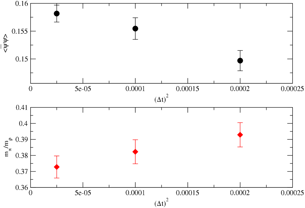
For the purpose of our simulations we implement the $R$ algorithm [11] with step-size $\Delta t=0.005$ and stopping condition $10^{-6}$. Figure 1 shows that our choice for the step-size allows us to measure physical quantities with an error due to finite step-size smaller than 2%, and that we are running in the stable regime of the $R$ algorithm. For the spectrum measurements we use box sources of size 2 and local sinks for all runs.

Our simulations examine the phase transition and the thermodynamic properties of QCD for volumes, temperatures, spatial lattice scales and quark masses similar to the already used in the $N_{t}=4$, 2-flavor thermodynamic studies on isotropic lattices [5]. We adjusted the bare parameters in the action so that the resulting physical anisotropy $\xi\approx 4$, while $a_{s}\approx 0.3$ fm and $m_{\pi}/m_{\rho}\approx 0.3$, which allowed the critical $N_{t}\approx 16$.

Another important step in tuning the bare parameters is choosing $\nu_{t}$ such that the relativistic properties of the anisotropic staggered action are restored. The velocity of light $c_{ts}$ is defined through the meson dispersion relation:

$$E_{t,{\rm phys}}^{2}(P_{s,{\rm phys}}) = \frac{E_{t,{\rm lat}}^{2}(0)}{a_{t}^{2}}+c_{ts}^{2}P^{2}_{s,{\rm lat}}\frac{1}{a_{s}^{2}},$$ (123)

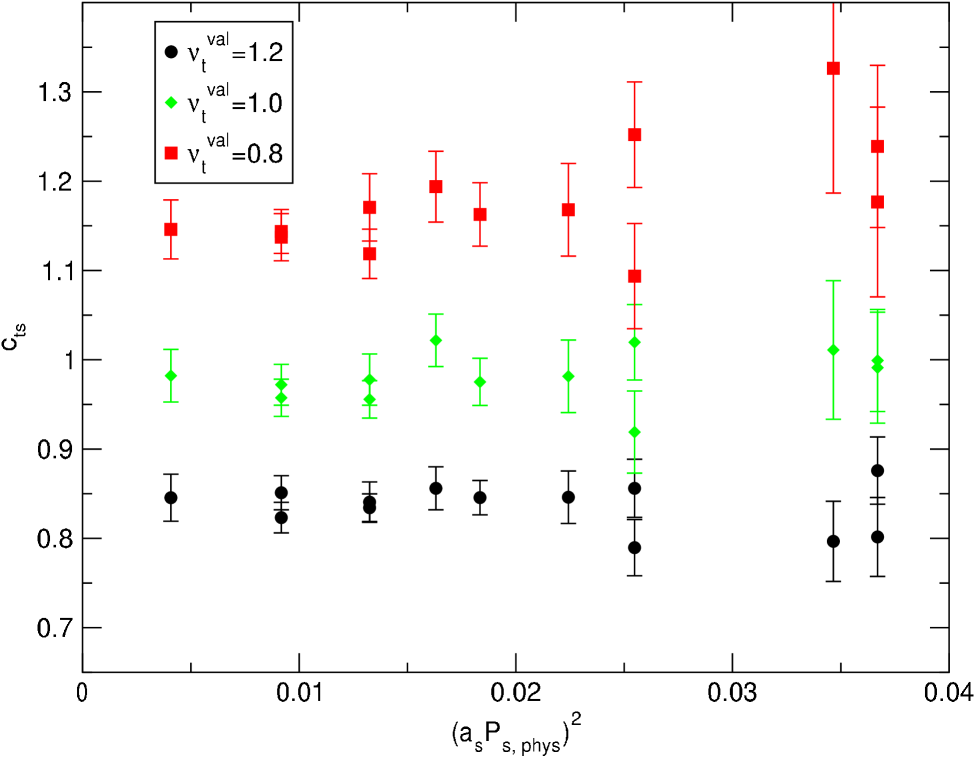
where $E$ and $P$ are the energy and the momentum of the meson, subscripts “lat” and “phys” refer to a quantity in lattice or physical units, and $s$ and $t$ whether it is measured in the spatial or temporal direction. We tune $\nu_{t}$, so that the velocity of light $c_{ts}(P_{s,{\rm phys}})\approx 1$. The velocity of light is calculated for the $\pi$ propagating in the temporal direction with a non-zero momentum for three valence values of this parameter, $\nu^{\rm val}_{t}=0.8$, 1.0 and 1.2 (the dynamical value is $\nu^{\rm dyn}_{t}=1.0$). Figure 2 demonstrates that the choice of $\nu^{\rm val}_{t}=1.0$ gives a velocity of light closest to 1.0 for the set of bare parameters $\beta=5.3$, $\xi_{o}=3.0$ and $m_{f}=0.008$.

In Table I we compare masses measured in the temporal and spatial directions for various combinations of $\nu^{\rm dyn}_{t}$ and $\nu^{\rm val}_{t}$. This shows that a 20% change in $\nu^{\rm dyn}_{t}$ has only a small effect compared to a similar change in $\nu^{\rm val}_{t}$. For the masses we measure the essential contribution comes from $\nu^{\rm val}_{t}$.

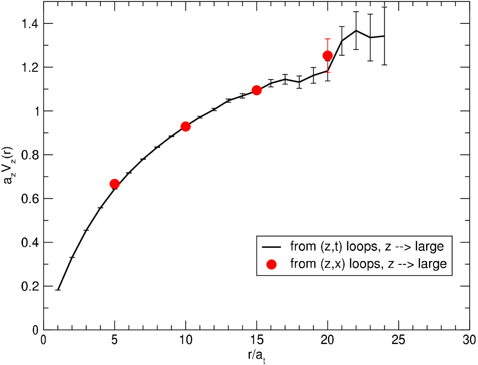
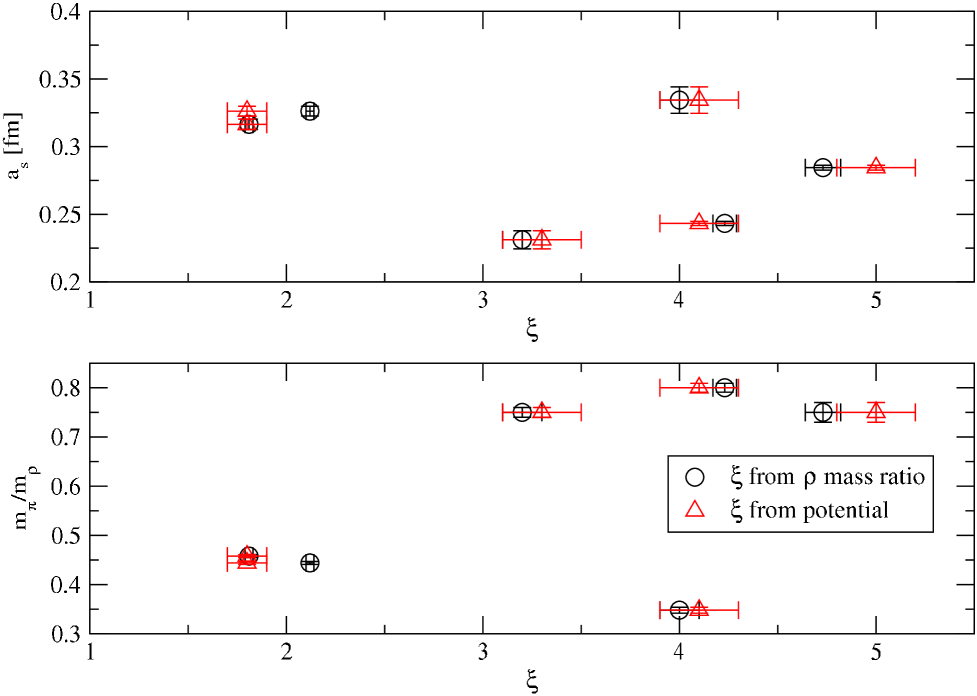
Table II, Table III and Table IV list all the zero temperature scale setting runs and the finite temperature runs that we have done. The anisotropy $\xi$ for each of the zero temperature runs is calculated from the ratio of the $\rho$ masses in the spatial and temporal directions. For runs 1–5 and 7, Table II, $\xi$ is determined from the matching of the static potentials as well (Figure 3 illustrates the matching technique [9]). The comparison between the two methods can be done examining Figure 4, which shows that they give reasonably close results.

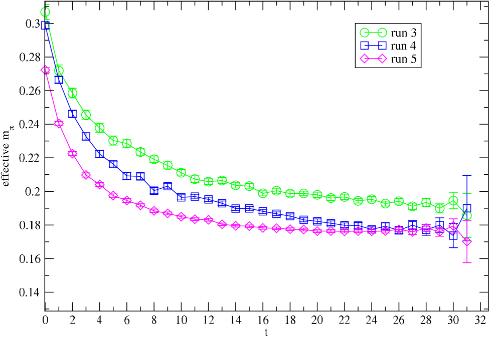
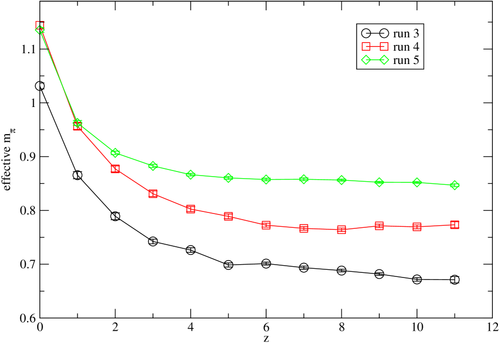
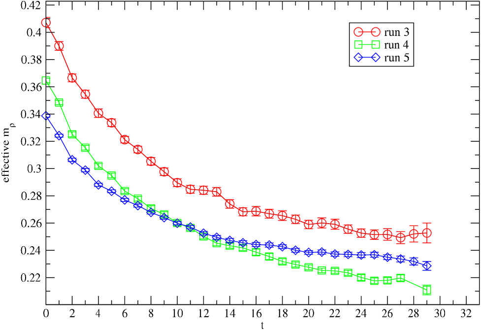
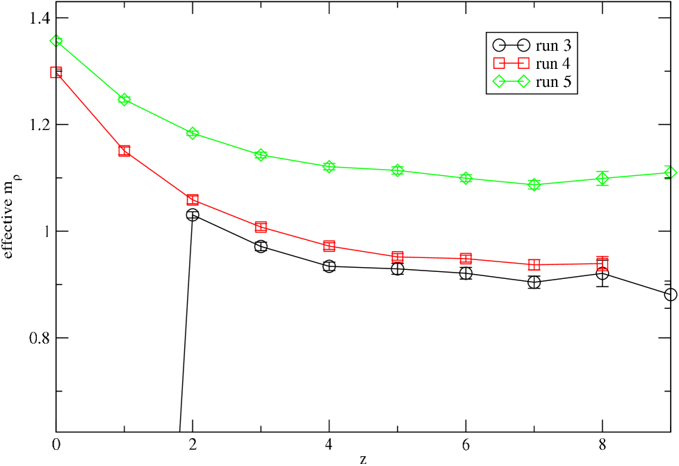
The quality of our data for all runs from Table II can be judged by studying the effective mass plots for $\pi$ and $\rho$. On Figure 5 through Figure 8 we show some typical effective mass plots. The effective mass at a given time or space slice is calculated from the values of the correlators at 2 neighboring points for $\pi$ and 4 for $\rho$, in order to determine all the parameters in the respective one and two cosh fitting forms. Ideally after some minimal time or space slice the effective mass plots should exhibit a plateau. For some effective mass plots determined from the spatial correlators the quality of the plateau is not high, especially for the runs with very coarse lattice spacing, which means that for those runs there are larger errors on the meson masses determined from the fits to all data points.

All the data which we used in the Karsch coefficients and the EOS determination is given in Table V.

IV Phase Transition

The finite temperature runs from Table III and Table IV correspond to two sweeps through the phase transition for two different anisotropies $\xi=4.0(1)$ and $\xi=4.8(3)$, with corresponding $a_{s}$ of $0.34(1)$ fm, and $0.354(9)$ fm and $(m_{\pi}/m_{\rho})^{temporal}$ of $0.33(1)$ and $0.325(8)$, respectively.

For each sweep through the transition region the temperature is changed only by changing $N_{t}$, while all other parameters are kept constant. We want to stress the fact that there are no scale changes between the different finite temperature runs from a group with a given anisotropy and that the scales change minimally between the two groups of runs belonging to the two different anisotropies.

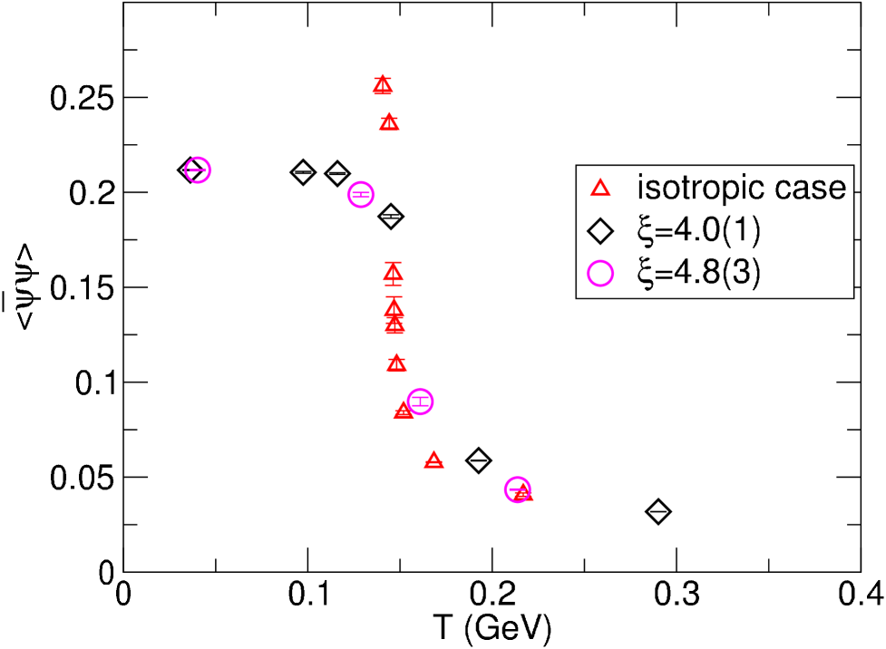
Figure 9 shows the temperature dependence of $\langle\overline{\psi}\psi\rangle$ in the critical region. From the data we can estimate $T_{c}\approx 150-160$ MeV. An interesting observations is that the shape of the transition is comparable in sharpness with the phase transition obtained in previous isotropic calculation [12, 13] also shown on the same figure. The isotropic data is from a dynamical staggered calculation with two fermion flavors on $16^{3}\times 4$ volume and $m_{f}=0.025$. The scale used to calculate the temperature in the isotropic case is from [5]. The differences between our anisotropic result and the isotropic one we attribute to the scaling violations in the latter which we have avoided in our fixed parameter scheme.

V Karsch Coefficients

To determine the EOS we need to know the Karsch coefficients which are involved in the analytic expressions Eq. (102) and Eq. (122). The values of these derivatives can be calculated using the physical quantities that we measure for each zero-temperature run : $a_{s}$, $\xi$, $R_{t}=(m_{\pi}^{2}/m_{\rho}^{2})^{\rm temporal}$ and $R_{st}=(m_{\pi}^{2}/m_{\rho}^{2})^{\rm spatial}/(m_{\pi}^{2}/m_{\rho}^{2})^{\rm temporal}$. We consider the bare parameters $\xi_{o}$, $\beta$, $m_{f}$ and $\nu_{t}$ to be functions of the above physical quantities, which allows those functions to be expanded in Taylor series around the physical quantities of a selected zero-temperature run as follows:

$$\Delta\xi_{o}(\xi,a_{s},R_{t},R_{st},\{\bf{c_{i}}\}) = c_{1}\Delta\xi+c_{2}\Delta a_{s}+c_{3}\Delta R_{t}+c_{4}\Delta R_{st}+\cdots$$ (124)

$$\Delta\beta(\xi,a_{s},R_{t},R_{st},\{\bf{d_{i}}\}) = d_{1}\Delta\xi+d_{2}\Delta a_{s}+d_{3}\Delta R_{t}+d_{4}\Delta R_{st}+\cdots$$ (125)

$$\Delta m_{f}(\xi,a_{s},R_{t},R_{st},\{\bf{e_{i}}\}) = e_{1}\Delta\xi+e_{2}\Delta a_{s}+e_{3}\Delta R_{t}+e_{4}\Delta R_{st}+\cdots$$ (126)

$$\Delta\nu_{t}(\xi,a_{s},R_{t},R_{st},\{\bf{f_{i}}\}) = f_{1}\Delta\xi+f_{2}\Delta a_{s}+f_{3}\Delta R_{t}+f_{4}\Delta R_{st}+\cdots,$$ (127)

where $\Delta\xi_{o}=\xi_{o}-\xi^{\prime}_{o}$, $\Delta\beta=\beta-\beta^{\prime}$, $\Delta m_{f}=m_{f}-m^{\prime}_{f}$, $\Delta\nu_{t}=\nu_{t}-\nu^{\prime}_{t}$, $\Delta\xi=\xi-\xi^{\prime}$, $\Delta a_{s}=a_{s}-a_{s}^{\prime}$, $\Delta R_{t}=R_{t}-R^{\prime}_{t}$, $\Delta R_{st}=R_{st}-R^{\prime}_{st}$. In the last definitions the primed quantities refer to the selected run around whose physical quantities the Taylor expansion is done. The derivatives $c_{i}$, $d_{i}$, $e_{i}$ and $f_{i}$, $i=(1,\dots,4$), are defined as:

$$\left(\begin{tabular}[]{cccc}$c_{1}$&$c_{2}$&$c_{3}$&$c_{4}$\\ $d_{1}$&$d_{2}$&$d_{3}$&$d_{4}$\\ $e_{1}$&$e_{2}$&$e_{3}$&$e_{4}$\\ $f_{1}$&$f_{2}$&$f_{3}$&$f_{4}$\\ \end{tabular}\right) = \left(\begin{tabular}[]{rrrr}\vspace{0.1cm} $\left.\frac{\partial\xi_{o}}{\partial\xi}\right|_{a_{s},R_{t},R_{st}}$&$\left.\frac{\partial\xi_{o}}{\partial a_{s}}\right|_{\xi,R_{t},R_{st}}$&$\left.\frac{\partial\xi_{o}}{\partial R_{t}}\right|_{\xi,a_{s},R_{st}}$&$\left.\frac{\partial\xi_{o}}{\partial R_{st}}\right|_{\xi,a_{s},R_{t}}$\\ \vspace{0.1cm} $\left.\frac{\partial\beta}{\partial\xi}\right|_{a_{s},R_{t},R_{st}}$&$\left.\frac{\partial\beta}{\partial a_{s}}\right|_{\xi,R_{t},R_{st}}$&$\left.\frac{\partial\beta}{\partial R_{t}}\right|_{\xi,a_{s},R_{st}}$&$\left.\frac{\partial\beta}{\partial R_{st}}\right|_{\xi,a_{s},R_{t}}$\\ \vspace{0.1cm} $\left.\frac{\partial m_{f}}{\partial\xi}\right|_{a_{s},R_{t},R_{st}}$&$\left.\frac{\partial m_{f}}{\partial a_{s}}\right|_{\xi,R_{t},R_{st}}$&$\left.\frac{\partial m_{f}}{\partial R_{t}}\right|_{\xi,a_{s},R_{st}}$&$\left.\frac{\partial m_{f}}{\partial R_{st}}\right|_{\xi,a_{s},R_{t}}$\\ \vspace{0.1cm} $\left.\frac{\partial\nu_{t}}{\partial\xi}\right|_{a_{s},R_{t},R_{st}}$&$\left.\frac{\partial\nu_{t}}{\partial a_{s}}\right|_{\xi,R_{t},R_{st}}$&$\left.\frac{\partial\nu_{t}}{\partial R_{t}}\right|_{\xi,a_{s},R_{st}}$&$\left.\frac{\partial\nu_{t}}{\partial R_{st}}\right|_{\xi,a_{s},R_{t}}$\\ \end{tabular}\right).$$ (136)

The Karsch coefficients, which are involved in the EOS, are the first two columns of the matrix of derivatives above. We assume that we can make linear fits to Eq. (124) through Eq. (127) for each zero-temperature run and minimize the $\chi^{2}_{i}$, $i=(1,\dots,4)$, for all of the zero-temperature runs at the same time. The $\chi^{2}_{i}$’s for the four fits are:

$$\chi^{2}_{1}(\{{\bf c_{i}}\}) = \sum_{r}[\Delta\xi_{o}^{r}-\Delta\xi_{o}^{r}(\xi^{r},a_{s}^{r},R_{t}^{r},R_{st}^{r},\{{\bf c_{i}}\})]^{2}/\sigma_{r}^{2}(\Delta\xi_{o}^{r})$$ (137)

$$\chi^{2}_{2}(\{{\bf d_{i}}\}) = \sum_{r}[\Delta\beta^{r}-\Delta\beta^{r}(\xi^{r},a_{s}^{r},R_{t}^{r},R_{st}^{r},\{{\bf d_{i}}\})]^{2}/\sigma_{r}^{2}(\Delta\beta^{r})$$ (138)

$$\chi^{2}_{3}(\{{\bf e_{i}}\}) = \sum_{r}[\Delta m_{f}^{r}-\Delta m_{f}^{r}(\xi^{r},a_{s}^{r},R_{t}^{r},R_{st}^{r},\{{\bf e_{i}}\})]^{2}/\sigma_{r}^{2}(\Delta m_{f}^{r})$$ (139)

$$\chi^{2}_{4}(\{{\bf f_{i}}\}) = \sum_{r}[\Delta\nu_{t}^{r}-\Delta\nu_{t}^{r}(\xi^{r},a_{s}^{r},R_{t}^{r},R_{st}^{r},\{{\bf f_{i}}\})]^{2}/\sigma_{r}^{2}(\Delta\nu_{t}^{r}).$$ (140)

In the above expressions the sums are over $r$, which labels each zero-temperature run and the bare parameters and physical quantities associated with it. This labeling is not the same as the numbering of the runs in Table II, where each run number refers to a specific set of dynamical bare parameters. Here the subscript $r$ labels a specific set of bare parameters which instead of $\nu^{\rm dyn}_{t}$ has the valence value of that parameter, since as we already showed, the $\nu^{\rm val}_{t}$ has the dominant contribution to the measured physical quantities. Hence in all formulae in this section the notation $\nu_{t}$ stands for the valence value of that parameter.

All expansions are taken around a given selected run, whose label is not shown. The minimization of $\chi^{2}_{1}$ for the first fit, Eq. (124) for example, leads to a matrix equation of the form

$$AC=V,$$ (141)

where

$$A = \left(\begin{tabular}[]{cccc}\vspace{0.2cm} $\sum_{r}\frac{\Delta\xi^{r}\Delta\xi^{r}}{\sigma_{r}^{2}(\Delta\xi_{o}^{r})}$&$\sum_{r}\frac{\Delta\xi^{r}\Delta a_{s}^{r}}{\sigma_{r}^{2}(\Delta\xi_{o}^{r})}$&$\sum_{r}\frac{\Delta\xi^{r}\Delta R_{t}^{r}}{\sigma_{r}^{2}(\Delta\xi_{o}^{r})}$&$\sum_{r}\frac{\Delta\xi^{r}\Delta R_{st}^{r}}{\sigma_{r}^{2}(\Delta\xi_{o}^{r})}$\\ \vspace{0.2cm} $\sum_{r}\frac{\Delta a_{s}^{r}\Delta\xi^{r}}{\sigma_{r}^{2}(\Delta\xi_{o}^{r})}$&$\sum_{r}\frac{\Delta a_{s}^{r}\Delta a_{s}^{r}}{\sigma_{r}^{2}(\Delta\xi_{o}^{r})}$&$\sum_{r}\frac{\Delta a_{s}^{r}\Delta R_{t}^{r}}{\sigma_{r}^{2}(\Delta\xi_{o}^{r})}$&$\sum_{r}\frac{\Delta a_{s}^{r}\Delta R_{st}}{\sigma_{r}^{2}(\Delta\xi_{o}^{r})}$\\ \vspace{0.2cm} $\sum_{r}\frac{\Delta R_{t}^{r}\Delta\xi^{r}}{\sigma_{r}^{2}(\Delta\xi_{o}^{r})}$&$\sum_{r}\frac{\Delta R_{t}^{r}\Delta a_{s}^{r}}{\sigma_{r}^{2}(\Delta\xi_{o}^{r})}$&$\sum_{r}\frac{\Delta R_{t}^{r}\Delta R_{t}^{r}}{\sigma_{r}^{2}(\Delta\xi_{o}^{r})}$&$\sum_{r}\frac{\Delta R_{t}^{r}\Delta R_{st}^{r}}{\sigma_{r}^{2}(\Delta\xi_{o}^{r})}$\\ \vspace{0.2cm} $\sum_{r}\frac{\Delta R_{st}^{r}\Delta\xi^{r}}{\sigma_{r}^{2}(\Delta\xi_{o}^{r})}$&$\sum_{r}\frac{\Delta R_{st}^{r}\Delta a_{s}^{r}}{\sigma_{r}^{2}(\Delta\xi_{o}^{r})}$&$\sum_{r}\frac{\Delta R_{st}^{r}\Delta R_{t}^{r}}{\sigma_{r}^{2}(\Delta\xi_{o}^{r})}$&$\sum_{r}\frac{\Delta R_{st}^{r}\Delta R_{st}^{r}}{\sigma_{r}^{2}(\Delta\xi_{o}^{r})}$\normalsize\end{tabular}\right),$$ (146)

$$V = \left(\begin{tabular}[]{c}\vspace{0.2cm} $\sum_{r}\frac{\Delta\xi_{o}^{r}\Delta\xi^{r}}{\sigma_{r}^{2}(\Delta\xi_{o}^{r})}$\\ \vspace{0.2cm} $\sum_{r}\frac{\Delta\xi_{o}^{r}\Delta a_{s}^{r}}{\sigma_{r}^{2}(\Delta\xi_{o}^{r})}$\\ \vspace{0.2cm} $\sum_{r}\frac{\Delta\xi_{o}^{r}\Delta R_{t}^{r}}{\sigma_{r}^{2}(\Delta\xi_{o}^{r})}$\\ \vspace{0.2cm} $\sum_{r}\frac{\Delta\xi_{o}^{r}\Delta R_{st}^{r}}{\sigma_{r}^{2}(\Delta\xi_{o}^{r})}$\\ \end{tabular}\right),$$ (151)

$$C = \left(\begin{tabular}[]{c}$c_{1}$\\ $c_{2}$\\ $c_{3}$\\ $c_{4}$\\ \end{tabular}\right),\normalsize$$ (156)

which we solve for $C$. In a similar way we find matrix equations for the rest of the derivatives from Eq. (125), Eq. (126) and Eq. (127).

To apply statistical analysis on our data from the zero-temperature runs, we divide the data into a set of jackknife blocks. The numerical procedure for the minimization of the $\chi^{2}_{i}$ functions can not be applied straightforwardly for the equations Eq. (137) through Eq. (140) since the standard deviations of the bare parameters, $\sigma_{r}^{2}(\dots)$, are not known from the beginning. Instead we employ an iterative scheme which consists of the following steps:

• Start by guessing initial values for all $\sigma_{r}^{2}(\dots)$’s.

  1. Determine the Karsch coefficients by solving the matrix equation: Eq. (141), and the similar equations derived from minimizing Eq. (138) through Eq. (140).

  2. Using the values of the Karsch coefficients from step 1 calculate numerically the linear part of the functions Eq. (124) through Eq. (127) on each jackknife block of data and by statistically analyzing them find new values for all $\sigma_{r}^{2}(\dots)$’s.

• Repeat steps 1 and 2 until the numerical result for the Karsch coefficients converges.

The success of this scheme depends on how well the functions Eq. (124) through Eq. (127) can be approximated by the linear part of the Taylor expansion, which is a measure of how “close” the physical quantities measured from each run are to the quantities of the selected run around which the expansion is made. To trust the consistency of the iterative scheme we checked the two step procedure with variety of random initial guesses for the $\sigma_{r}^{2}(\dots)$’s, which reproduced the same final results.

The numerical results for the Karsch coefficients from expansion around runs 7 and 8 from Table II, obtained via the the method described above, are summarized in Tables VII and  VIII. The quoted errors are calculated using the jackknife method. Our results show larger errors on the Karsch coefficients which are derivatives with respect to $a_{s}$ than the errors on those coefficients that are derivatives with respect to $\xi$. A possible explanation of that difference could be that the specific parameter space that we explored in our zero-temperature runs does not allow a better resolution of some of the Karsch coefficients either because it is too limited (we need more runs and more statistics on each of them to improve the quality of mass fits) or because the “points” in that space (the zero-temperature runs) are not distributed in a favorable way around the run around which we are making the expansion, or both.

VI Equation of State

In the previous section we described the procedure which allows us to calculate the Karsch coefficients needed to determine the QCD equation of state (Eq. (102) and Eq. (122)).

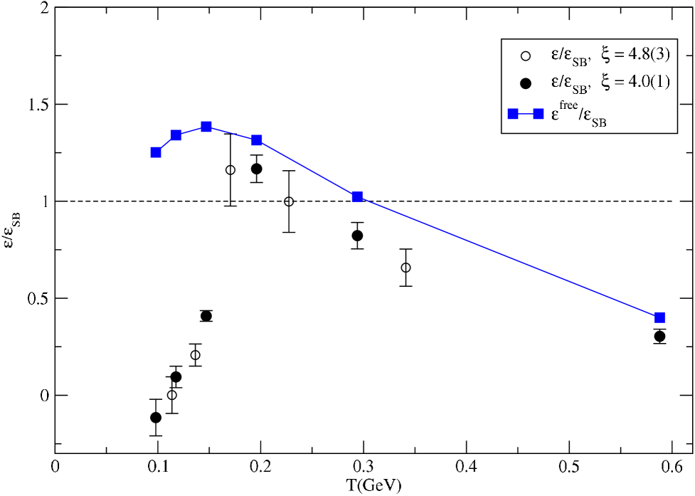
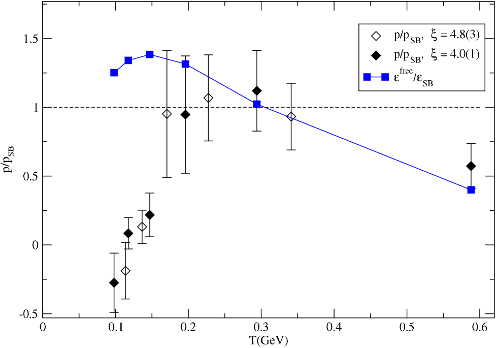
As stressed before in Section IV we have two groups of finite temperature runs listed in Tables III and IV , for each of which we are changing the temperature by only varying $N_{t}$ and keeping the underlying physics scales fixed. Figures 10 and 11 show the numerical results for the energy density and pressure for both groups of runs corresponding to anisotropies $\xi=4.0(1)$ and $4.8(3)$. The data is normalized to the continuum Stefan-Boltzmann values of the EOS for an ideal relativistic gas for $SU(N_{c})$ color with $N_{f}$ quark flavors, which are

$$\frac{\varepsilon_{\rm SB}}{T^{4}} = \frac{\pi^{2}}{15}(N_{c}^{2}-1+\frac{7}{4}N_{c}N_{f})\approx 12.1725$$ (157)

and

$$\frac{p_{\rm SB}}{T^{4}} = \frac{\varepsilon_{\rm SB}}{3T^{4}}.$$ (158)

The errors on the pressure are significantly larger than the errors on the energy due to the large errors on those of the Karsch coefficients which are derivatives with respect to $a_{s}$ and are involved only in Eq. (122) for the pressure. The comparison with the free lattice theory (squares) gives an explanation of the prominent drop off of $\varepsilon$ and $p$ in the high temperature sector – simply a consequence of the lattice high momentum cut-off. The high momentum mode contribution to the EOS becomes dominant with the increase of the temperature, which means that at a coarse lattice spacing a high proportion of relevant modes are simply excised. Including improvements to the spatial parts of the staggered fermion action would be a natural step to reduce those lattice artifacts for high temperatures.

Our results for the EOS are comparable with the isotropic case [14] in the temperature region up to 0.3 GeV for which the cited reference has data. The errors on the energy density are comparable with the errors in that isotropic study, or smaller with enough statistics, on the other hand the errors on pressure are larger due to the reasons stated above.

VII Note on Flavor Symmetry Improvement

In the continuum and chiral limits the spontaneous symmetry breaking of $SU(4)_{A}\otimes SU(4)_{V}$ in the staggered action, yields 15 Goldstone pions. On the lattice the violation of the flavor symmetry leaves us with the remnant $U(1)_{A}\otimes U(1)_{V}$ and only one true Goldstone pion. The local pions in the staggered formulation, which fall into 7 irreducible representations, are not degenerate any more due to the $O(a^{2})$ flavor symmetry breaking. However the introduction of anisotropy on the lattice makes the lattice spacing in the temporal direction much smaller than the spatial one and hence we expect to see an improvement in the flavor symmetry.

We choose $\Delta_{\pi}=(m_{\pi_{2}}-m_{\pi})/m_{\rho}$, where $\pi_{2}$ is the second local staggered pion, as a quantitative measure of the flavor symmetry breaking in the spatial and temporal directions. The data in Table VI shows that in the temporal direction for all runs $\Delta_{\pi}$ is smaller than its value in the spatial direction, which means that we are seeing improvement of the flavor symmetry as $a_{t}$ becomes finer. Especially for run 4, the $\pi$ and $\pi_{2}$ look virtually degenerate.

We expect that the anisotropy has a similar effect on the rest of the pions, although we have not investigated numerically how the various mass splittings between them are affected by the decrease of $a_{t}$.

VIII Conclusions

We have studied the thermodynamic properties of full QCD with 2-flavors of staggered fermions on anisotropic lattices. In our calculations we have employed a fixed parameter scheme in which we keep the bare parameters constant and change the temperature by varying only the number of the temporal slices $N_{t}$. This allowed us to study the phase transition for staggered fermions with fixed physics scales. It appears to be comparably as sharp as the transition in the isotropic case.

We have calculated non-perturbatively the Karsch coefficients from series of zero-temperatures runs and applied them in the determination of the EOS. Those of the Karsch coefficients which are derivatives with respect to $a_{s}$ have significant errors which are most probably due to the limited set of data used in their determination. They respectively give rise to large uncertainties in the calculation of the pressure.

The high temperature behavior of the quark-gluonic system was found to be strongly influenced by the underlying lattice cut-off, which gives a maximum temperature at which our anisotropic EOS should represent continuum physics. However the fixed parameter scheme combined with a spatially improved anisotropic staggered action might give a much better result in the high temperature region.

The anisotropic approach naturally reduces the finite lattice spacing errors associated with $a_{t}$ and accounts for an improvement of the flavor symmetry for particles propagating in the temporal direction.

It is interesting to mention that our results do not show a pronounced negative pressure problem in the confined phase as it has been found in previous EOS calculations using the derivative method with perturbatively calculated Karsch coefficients. However, considering the generally large statistical errors on the pressure in our calculation, we could not entirely exclude the possibility of such a problem being unveiled at low temperatures in a calculation with reduced statistical errors.

TABLE I.: Meson masses for run 1 and 2, Table II, measured with different valence and dynamical $\nu_{t}$’s. The comparison shows that the main contribution to the masses comes from $\nu^{\rm val}_{t}$. Notations $S$ and $T$ stand for spatial and temporal directions of measurement.

run	$\nu_{t}^{\rm dyn}$	$\nu_{t}^{\rm val}$	$m_{\pi}$, T	$m_{\pi}$, S	$m_{\rho}$, T	$m_{\rho}$, S
1	1.0	1.0	0.31309(28)	0.57846(83)	0.6853(63)	1.218(29)
2	1.2	1.0	0.31023(42)	0.57677(46)	0.6897(54)	1.257(15)
2	1.2	1.2	0.26761(35)	0.58299(49)	0.6030(43)	1.232(32)

TABLE II.: Parameters of zero-temperature calculations. All runs except run 2 have $\nu^{\rm dyn}_{t}=1.0$. Run 2 has $\nu^{\rm dyn}_{t}=1.2$.

run	volume	traj.	$\beta$	$\xi_{o}$	$m_{f}$
1	$16^{3}\times 32$	5800	5.425	1.5	0.025
2	$16^{2}\times 24\times 32$	5100	5.425	1.5	0.025
3	$16^{2}\times 24\times 64$	1300	5.695	2.5	0.025
4	$16^{2}\times 24\times 64$	1400	5.725	3.44	0.025
5	$16^{2}\times 24\times 64$	3400	5.6	3.75	0.025
6	$16^{2}\times 24\times 64$	4300	5.286	3.427	0.00394
7	$16^{2}\times 24\times 64$	3200	5.3	3.0	0.008
8	$16^{2}\times 24\times 64$	3000	5.29	3.4	0.0065

TABLE III.: Parameters of finite temperature calculations with $\xi=4.0(1)$. All runs have $\nu^{\rm dyn}_{t}=1.0$.

run	volume	traj.	$\beta$	$\xi_{o}$	$m_{f}$
1	$16^{3}\times 24$	8000	5.3	3.0	0.008
2	$16^{3}\times 20$	9800	5.3	3.0	0.008
3	$16^{3}\times 16$	21600	5.3	3.0	0.008
4	$16^{3}\times 12$	9100	5.3	3.0	0.008
5	$16^{3}\times 8$	5500	5.3	3.0	0.008
6	$16^{3}\times 4$	25900	5.3	3.0	0.008

TABLE IV.: Parameters of finite temperature calculations with $\xi=4.8(3)$. All runs have $\nu^{\rm dyn}_{t}=1.0$.

run	volume	traj.	$\beta$	$\xi_{o}$	$m_{f}$
1	$16^{3}\times 24$	1400	5.29	3.4	0.0065
2	$16^{3}\times 20$	2700	5.29	3.4	0.0065
3	$16^{3}\times 16$	8900	5.29	3.4	0.0065
4	$16^{3}\times 12$	6200	5.29	3.4	0.0065
5	$16^{3}\times 8$	3600	5.29	3.4	0.0065

TABLE V.: All zero-temperature data used to determine the Karsch coefficients from fits to Eq. (124) – Eq. (127). The run index in the first column corresponds to the run number of Table II, which lists the run parameters. Notations $S$ and $T$ stand for spatial and temporal directions of measurement. $R_{t}$ and $R_{st}$ are defined in Section V.

run	$\nu_{t}^{\rm val}$	$\xi$	$m_{\pi},T$	$m_{\pi},S$	$m_{\rho},T$	$m_{\rho},S$	$R_{t}$	$R_{st}$
1	1.0	1.778(46)	0.31309(28)	0.57846(83)	0.6853(63)	1.218(29)	0.2087(39)	1.080(56)
2	0.8	1.495(21)	0.37050(41)	0.56794(39)	0.8227(69)	1.230(14)	0.2028(33)	1.051(29)
2	1.0	1.822(24)	0.31023(42)	0.57677(46)	0.6897(54)	1.257(15)	0.2023(32)	1.041(28)
2	1.2	2.043(56)	0.26761(35)	0.58299(49)	0.6030(43)	1.232(32)	0.1970(28)	1.137(62)
3	0.8	2.767(41)	0.2451(10)	0.6710(50)	0.3144(34)	0.870(11)	0.608(12)	0.979(27)
3	1.0	3.637(80)	0.1925(26)	0.6774(48)	0.2547(39)	0.926(13)	0.571(16)	0.936(37)
3	1.2	3.273(76)	0.2094(39)	0.6732(47)	0.2716(54)	0.889(13)	0.594(12)	0.966(31)
4	0.8	3.722(41)	0.2048(11)	0.7643(24)	0.2481(28)	0.9235(58)	0.681(16)	1.005(23)
4	1.0	4.295(54)	0.17811(84)	0.7699(24)	0.2210(23)	0.9493(62)	0.649(14)	1.013(27)
4	1.2	4.888(70)	0.15955(89)	0.7786(23)	0.1980(22)	0.9680(65)	0.649(14)	0.997(28)
5	0.8	3.990(34)	0.20466(65)	0.8456(27)	0.2706(18)	1.0796(74)	0.5721(80)	1.072(18)
5	1.0	4.658(35)	0.17661(76)	0.8540(20)	0.2382(13)	1.1096(88)	0.5497(80)	1.078(16)
5	1.2	5.260(46)	0.15637(69)	0.8624(22)	0.21374(99)	1.1242(90)	0.5352(74)	1.099(21)
6	1.0	4.60(21)	0.07413(25)	0.36410(77)	0.2811(39)	1.294(51)	0.0695(20)	1.14(10)
7	0.8	3.57(30)	0.13273(42)	0.47488(42)	0.3777(51)	1.35(11)	0.1235(33)	1.00(17)
7	1.0	4.03(14)	0.11280(51)	0.47682(38)	0.3274(39)	1.320(49)	0.1187(29)	1.099(77)
7	1.2	4.903(75)	0.09800(44)	0.47950(36)	0.2857(34)	1.401(15)	0.1177(28)	0.996(30)
8	1.0	4.80(28)	0.09517(39)	0.46121(58)	0.2821(56)	1.354(57)	0.1138(45)	1.02(10)

TABLE VI.: The second local staggered pion masses $m_{\pi_{2}}$ and $\Delta_{\pi}=(m_{\pi_{2}}-m_{\pi})/m_{\rho}$ from the zero-temperature runs with parameters given in Table II. The run index in the first column corresponds to the run number of Table II. Notations $S$ and $T$ stand for spatial and temporal directions of measurement. For large values of the anisotropy $\xi$, $\Delta_{\pi}$ in the temporal direction is significantly smaller than the corresponding value in the spatial direction, for some runs even consistent with zero.

run	$\nu_{t}^{\rm val}$	$\xi$	$m_{\pi_{2}}$, $T$	$m_{\pi_{2}}$, $S$	$\Delta_{\pi}$, $T$	$\Delta_{\pi}$, $S$
1	1.0	1.778(46)	0.4605(37)	1.109(25)	0.2151(45)	0.436(24)
2	0.8	1.495(21)	0.5803(75)	1.243(92)	0.2551(89)	0.549(79)
2	1.0	1.822(24)	0.4729(54)	1.17(12)	0.2359(75)	0.475(95)
2	1.2	2.043(56)	0.3996(31)	1.119(32)	0.2188(54)	0.435(27)
3	0.8	2.767(41)	0.2484(18)	0.7462(75)	0.0106(56)	0.0864(87)
3	1.0	3.637(80)	0.1948(18)	0.779(11)	0.0091(65)	0.110(10)
3	1.2	3.273(76)	0.2115(40)	0.7592(80)	0.008(11)	0.0967(89)
4	0.8	3.722(41)	0.2071(11)	0.8379(71)	0.0094(42)	0.0797(77)
4	1.0	4.295(54)	0.17931(97)	0.8418(66)	0.0054(47)	0.0757(70)
4	1.2	4.888(70)	0.1598(10)	0.8594(69)	0.0011(59)	0.0834(71)
5	0.8	3.990(34)	0.20853(83)	0.9962(78)	0.0143(29)	0.1395(68)
5	1.0	4.658(35)	0.17954(77)	1.0125(79)	0.0123(31)	0.1428(70)
5	1.2	5.260(46)	0.15877(75)	1.0380(84)	0.0112(33)	0.1562(74)
6	1.0	4.60(21)	0.0956(14)	0.58(11)	0.0762(53)	0.168(85)
7	0.8	3.57(30)	0.1693(14)	1.30(36)	0.0969(42)	0.61(26)
7	1.0	4.03(14)	0.1410(11)	1.24(16)	0.0861(42)	0.58(12)
7	1.2	4.903(75)	0.1213(13)	1.181(79)	0.0816(54)	0.501(56)
8	1.0	4.80(28)	0.1142(14)	1.54(21)	0.0674(54)	0.80(16)

TABLE VII.: Karsch coefficients from fitting the data to the liner part of the Taylor expansion around run 7, Table II, with $\xi=4.0(1)$. The order of the coefficients is the same as in the matrix in Eq. (136). Each row is obtained from the fitting procedure independently from the other rows and the $\chi^{2}$’s per degree of freedom for each fit is respectively 1.7, 1.0, 1.8 and 0.7.

0.61(6)	9.6(6.2)	2.0(1.1)	0.3(2.0)
-0.017(7)	-1.5(1.1)	0.5(2)	-0.03(28)
-0.0062(4)	0.18(5)	0.068(4)	-0.003(15)
0.04(5)	-5.6(4.8)	-0.7(8)	1.1(1.4)

TABLE VIII.: Karsch coefficients from fitting the data to the liner part of the Taylor expansion around run 8, Table II, with $\xi=4.8(3)$. The order of the coefficients is the same as in the matrix in Eq. (136). Each row is obtained from the fitting procedure independently from the other rows and the $\chi^{2}$’s per degree of freedom for each fit is 1.4, 0.7, 2.3 and 0.9.

0.59(6)	9.2(6.2)	2.2(1.0)	0.7(1.8)
-0.015(6)	-1.0(4)	0.58(8)	0.02(8)
-0.0050(8)	0.11(7)	0.05(1)	0.02(2)
0.06(3)	-5.0(4.1)	-0.8(7)	0.8(1.2)

FIG. 1.: Dependence of physical quantities on the step-size $\Delta t$ for volume $8^{3}\times 32$, $\beta=5.35$, $\xi_{o}=3.5$, $\nu^{\rm dyn}_{t}=\nu^{\rm val}_{t}=1.0$ and $m_{f}=0.006$. Trajectories per point about 900. We simulate at $\Delta t=0.005$.

FIG. 2.: Tuning of the velocity of light $c_{ts}$ using the dispersion relation in section III for $\pi$. The run parameters are $\beta=5.3$, $\xi_{o}=3.0$, $m_{f}=0.008$, $\nu^{\rm dyn}_{t}=1.0$; Measurements are done at $\nu^{\rm val}_{t}=0.8$, 1.0 and 1.2. Square of the spatial momentum in lattice units $a_{s}P_{s,phys}$ is plotted on the horizontal axis. The choice of $\nu^{\rm val}_{t}=1.0$ gives velocity of light closest to unity for that set of parameters.

FIG. 3.: Potential matching technique applied to static potentials measured from Wilson loops in the $(z,x)$ and the $(z,t)$ planes for run 5, Table II. On this plot they are shown after they are made to match by dividing the abscissa for the potential measured from the $(z,x)$ loops by the anisotropy $\xi\approx 5$, so that $V_{z}(\xi a_{t}n)=V_{z}(a_{s}n)$.

FIG. 4.: Scatter plots for zero-temperature runs 1–5 and 7, Table II. The renormalized anisotropy $\xi$ is calculated both from the $\rho$ mass ratio in the spatial and temporal directions and from static potential matching. The two methods give the same anisotropy but the errors for the potential matching results are larger.

FIG. 5.: Effective mass plot for $\pi$ propagating in temporal direction. Run parameters are as in Table II and data is measured at the dynamical value of $\nu_{t}$.

FIG. 6.: Effective mass plot for $\pi$ propagating in spatial direction. Run parameters are as in Table II and data is measured at the dynamical value of $\nu_{t}$.

FIG. 7.: Effective mass plot for $\rho$ propagating in temporal direction. Run parameters are as in Table II and data is measured at the dynamical value of $\nu_{t}$.

FIG. 8.: Effective mass plot for $\rho$ propagating in spatial direction. Run parameters are as in Table II and data is measured at the dynamical value of $\nu_{t}$.

FIG. 9.: The temperature dependence of $\langle\overline{\psi}\psi\rangle$ in the region of $T_{c}$. Points from anisotropic runs with a common symbol have the same anisotropy and physics scales. The isotropic data is shown for comparison. From the critical region we estimate $T_{c}\approx 150$ – 160 MeV.

FIG. 10.: Energy in units of the Stefan-Boltzmann limit and a comparison with the free lattice theory (squares). The Stefan-Boltzmann law for a relativistic ideal gas for $SU(N_{c})$ color with $N_{f}$ quark flavors in the continuum is $\frac{\varepsilon_{\rm SB}}{T^{4}}=\frac{\pi^{2}}{15}(N_{c}^{2}-1+\frac{7}{4}N_{c}N_{f})\approx 12.1725$ for $N_{c}=3$ and $N_{f}=2$. Points with a common symbol share the same anisotropy and the same physics scales at all temperatures.

FIG. 11.: Pressure in units of the Stefan-Boltzmann limit and a comparison with the free lattice theory (squares). The Stefan-Boltzmann law for a relativistic ideal gas for $SU(3)$ color with $N_{f}=2$ quark flavors in the continuum gives $\frac{p_{\rm SB}}{T^{4}}=\frac{\varepsilon_{\rm SB}}{3T^{4}}$. Points with a common symbol share the same anisotropy and the same physics scales at all temperatures.

REFERENCES

• [1] F. Karsch, Nucl. Phys. B205[FS5], 285 (1982).
• [2] G. Burgers et al., Nucl. Phys. B304, 587 (1988).
• [3] R. C. Trinchero, Nucl. Phys. B227, 61 (1983).
• [4] F. Karsch and I. O. Stamatescu, Phys. Lett. B227, 153 (1989).
• [5] T. Blum et al., Nucl. Phys. (Proc. Suppl.) B34, 320 (1994); Phys. Rev. D51, 5153 (1995).
• [6] S. Huang et al., Phys. Rev. D42, 2864 (1990).
• [7] J. Engels et al., Phys. Lett. B252, 625 (1990).
• [8] QCD-TARO Collaboration: Ph. de Forcrand et al., Phys. Rev. D63:054501 (2001).
• [9] T. Klassen, Nucl. Phys. B533, 557 (1998).
• [10] L. Susskind, Phys. Rev. D16, 3031 (1977).
• [11] S. Gottlieb et al., Phys. Rev. D35, 2531 (1987).
• [12] A. Vaccarino, Nucl. Phys. (Proc. Suppl.) B20, 263 (1991).
• [13] ”Numerical Studies of the QCD Finite Temperature Phase Transition with Two and Three Flavors of Light Quarks”, Ph.D. thesis by A. Vaccarino, Columbia University (1991).
• [14] MILC Collaboration: C. W. Bernard et al., Phys. Rev. D55, 6861 (1997).