Lattice QCD with fixed topology

Hidenori Fukaya

Yukawa Institute for Theoretical Physics,
Kyoto University, Kyoto 606-8502, Japan

A Dissertation in candidacy for

the degree of Doctor of Philosophy

Abstract

The overlap Dirac operator, which satisfies the Ginsparg-Wilson relation, realizes exact chiral symmetry on the lattice. It also avoids fermion doubling but its locality and smoothness are subtle. In fact, the index theorem on the lattice implies that there are certain points where the overlap Dirac operator has discontinuities. Aside from the theoretical subtleties, this non-smoothness also raises practical problems in numerical simulations, especially in $N_{f}\neq 0$ full QCD case. One must carefully calculate the lowest eigenvalue of the Dirac operator at each hybrid Monte Carlo step, in order to catch sudden jumps of the fermion determinant on the topology boundaries (reflection/refraction). The approximation of the sign function, which is a crucial point in implementing the overlap Dirac operator, gets worse near the discontinuities.

A solution may be to concentrate on a fixed topological sector in the full theory. It is known that an “admissibility” condition, which suppress small plaquette values, preserves topology of the gauge fields and improves the locality of the overlap Dirac operator at the same time. In this thesis, we test a gauge action which automatically generates “admissible” configurations, as well as (large) negative mass Wilson fermion action which would also keep the topology. The quark potential and the topology stability are investigated with different lattice sizes and different couplings. Then we discuss the effects of these new approaches on the numerical cost of the overlap fermions.

The results of quenched QCD in the $\epsilon$-regime are also presented as an example of the lattice studies with fixed topology. Remarkable quark mass and topology dependences of meson correlators allow us to determine the fundamental parameters of the effective theory, in which the exact chiral symmetry with the Ginsparg Wilson relation plays a crucial role.

1 Introduction

Lattice QCD has played an important role in elementary particle physics, in particular, in studying the low energy dynamics of hadrons. One can nonperturbatively calculate hadron masses or decay constants with Monte Carlo simulations. As compensation, however, the lattice discretization of space-time spoils a lot of symmetries of the gauge theory. Violation of the translational symmetry would be an easiest example.

It is well known that chiral symmetry is not compatible with the absence of fermion doubling, due to the periodic properties of the lattice Dirac operator in momentum space [1, 2]. A popular prescription to avoid the appearance of unphysical modes, or doublers, is adding a so-called Wilson term [3] to the naive subtraction operator;

$$D_{W} = \frac{1}{2}\gamma_{\mu}(\nabla_{\mu}+\nabla_{\mu}^{*})-\frac{ra}{2}\nabla_{\mu}^{*}\nabla_{\mu}.$$ (1.1)

where $r$ is Wilson parameter (we set $r=1$.). This term gives a large mass to the doublers which are decoupled from the theory. The Wilson term, however, violates chiral symmetry. A well known difficulty with Wilson fermion is renormalization. The complicated operator mixing, additive quark mass corrections, have to be calculated. Actually these are obstacles to obtain reliable numerical data, especially in the chiral limit.

With the overlap Dirac operator [4, 5], as well as the other Dirac operators [6, 7, 8, 9, 10], which satisfies the Ginsparg-Wilson relation [11], one can construct lattice gauge theories which have the exact chiral symmetry [12]. Although the good chiral behaviors in applying the overlap operator to QCD are reported in both theoretical and numerical studies, its locality properties and smoothness with respect to the gauge fields are not so obvious. Since it has a term proportional to $1/\sqrt{a^{2}H_{W}^{2}}\equiv 1/\sqrt{(\gamma_{5}(aD_{W}-1-s))^{2}}$, where $s$ is a fixed parameter in the region $|s|<1$, the near zero modes of $H_{W}$ can contaminate the locality or smoothness properties. In fact, it is not difficult to see that there exist some points where the overlap Dirac operator, $aD$, is not smooth by noting the fact that the index of $aD$ can take integer values only. Also practically, near zero modes of $H_{W}$ causes some problems in the numerical simulations. Small eigen-modes of $|H_{W}|$ lower the convergence of polynomial or rational expansion of $1/\sqrt{a^{2}H_{W}^{2}}$. For example, to keep a certain accuracy, the order of the Chebyshev polynomial has to be proportional to $1/\lambda_{\mathrm{min}}$, where $\lambda_{\mathrm{min}}$ is the minimum eigenvalue of $|H_{W}|$. In full QCD with the dynamical overlap fermion [13, 14, 15, 16, 17, 18, 19, 20, 21, 22, 23, 24], one would have to carefully perform the hybrid Monte Carlo [25] updating near $H_{W}\sim 0$ points since sudden changes of the trajectories, reflection or refraction, should occur due to sudden jumps of the fermion determinant. Thus, at least, the smallest eigenvalue of $H_{W}$ always needs to be monitored in conventional methods of lattice QCD simulations, which is very time consuming and it is known that reflection/refraction itself has systematic errors when one employs the pseudo-fermion method [23]. Because of these difficulties, no lattice QCD study with the $N_{f}\neq 0$ overlap Dirac fermions has been done except for the cases with a very small lattice size.

An interesting solution might be prohibiting the topology change along the simulations. It is known that under a smoothness condition on the plaquette variables [26, 27, 28, 29],

$$||1-P_{\mu\nu}(x)||<\epsilon\;\;\;\;\mbox{for all ($x$, $\mu,\nu)$},$$ (1.2)

which is called the “admissibility” bound, any eigenvalues of $H_{W}$ are non-zero (we denote $|H_{W}|>0$) and the topological charge can be conserved if $\epsilon$, which is a fixed number, is sufficiently small [29, 30]. Furthermore, when $|H_{W}|>0$, the locality is also guaranteed. The “admissibility” condition, Eq.(1.2), is automatically satisfied if one takes a type of gauge action which diverges when $||1-P_{\mu\nu}(x)||\to\epsilon$ [31, 32, 33, 34, 35, 36, 37, 38].

Topology transitions can also be suppressed by including the factor, $\det H_{W}^{2}$, in the functional integral [39]. The inclusion of this factor was previously considered in a study of domain-wall fermions [40, 41, 42], where the aim was to reduce the effects of the finiteness of the lattice in the 5th dimension. If any eigenvalue approaches near $H_{W}=0$ along the simulation, the determinant, $\det H_{W}^{2}$, would give a very small Boltzmann weight, and such a trajectory would be rejected. Since $\det H_{W}^{2}=\det(D_{W}-(1+s)/a)^{2}$ is equivalent to $N_{f}=2$ Wilson fermion determinant with a negative cutoff-scale mass, it would not have any effects on the low energy physics. Moreover, the numerical cost of this determinant is expected to be much smaller than that of the dynamical overlap fermions.

What can we do with the configurations in a fixed topological sector ? A straightforward application would be QCD in the so-called $\epsilon$-regime [43, 44, 45, 46, 47, 48], where the linear extent of the space-time is smaller than the pion Compton wave length $L\ll 1/m_{\pi}$. In this regime (though it is an unphysical small-volume situation), it is believed that one would be able to evaluate the pion decay constant and the chiral condensates, which are the fundamental parameters of the chiral perturbation theory (ChPT)[49, 50]. They should be evaluated in lattice QCD studies without taking the large volume limit, since the finite volume effects are already involved on the ChPT side [51, 52, 53, 54, 55, 56, 57, 58, 59, 60, 61, 62, 63, 64, 65, 66].

In this thesis, we study

1. The practical feasibility of the topology conserving gauge action which keeps the “admissibility” bound, Eq.(1.2), as well as the Wilson fermion action with a large negative mass. A careful analysis on the gluonic quantity and comparison with that with the standard plaquette action have to be done.

2. How much stable the topological charge can be, with these topology conserving actions.

3. Their effect on the numerical cost of the overlap Dirac operator.

4. The determination of the low energy constants of quenched chiral perturbation theory in the $\epsilon$-regime in a fixed topological sector. This study would be helpful when $N_{f}\neq 0$ simulations with the dynamical overlap fermion are done in the future works.

We start with the theoretical details on the overlap Dirac operator and topology of the lattice gauge fields in Sec. 2. The technical issues of our numerical study is presented in Sec. 3. To test their practical application, the static quark potential with different couplings and $\epsilon$ and with/without the negative mass Wilson fermions is investigated (Sec. 4). We study the parameter dependence of the topological charge stability in Sec. 5. Then the effects on the overlap Dirac operator are discussed in Sec. 6. The numerical result of quenched lattice QCD in the $\epsilon$-regime is presented in Sec. 7. Conclusions and discussions are given in Sec. 8.

The main papers contributed to this thesis are

• H. Fukaya, S. Hashimoto, T. Hirohashi, K. Ogawa and T. Onogi, “Topology conserving gauge action and the overlap-Dirac operator,” Phys. Rev. D 73, 014503 (2006) [arXiv:hep-lat/0510116] [37],

• H. Fukaya, S. Hashimoto and K. Ogawa, “Low-lying mode contribution to the quenched meson correlators in the epsilon-regime,” Prog. Theor. Phys.  114 (2005) 451 [arXiv:hep-lat/0504018][59].

Refer also [31, 32] which are similar studies in 2-dimensions as a good test ground.

2 The overlap Dirac operator and topology

The overlap Dirac operator [4, 5] is defined by

$$D=\frac{1}{\bar{a}}\left(1+\gamma_{5}\frac{aH_{W}}{\sqrt{a^{2}H_{W}^{2}}}\right),\;\;\;\bar{a}=\frac{a}{1+s},\;\;\;aH_{W}=\gamma_{5}(aD_{W}-1-s),$$ (2.1)

which satisfies the Ginsparg-Wilson relation [11]

$$\gamma_{5}D+D\gamma_{5}=\bar{a}D\gamma_{5}D,$$ (2.2)

and $\gamma_{5}$-hermiticity $D^{\dagger}=\gamma_{5}D\gamma_{5}$. Here $s$ is a real parameter which satisfies $|s|<1$. The Dirac operator Eq.(2.1) is gauge covariant and has no fermion doubling, as one can see in the Fourier transform of $aD$ in the free case ;

$$a\tilde{D}(p) = 1-\left(1-\frac{1}{2}a^{2}\hat{p}^{2}-ia\gamma_{\mu}\tilde{p_{\mu}}\right)\left(1+\frac{1}{2}a^{4}\sum_{\mu<\nu}\hat{p_{\nu}}\hat{p_{\nu}}\right)^{-1/2}\sim ia\gamma_{\mu}p_{\mu}+O((ap_{\mu})^{2}),$$

$$\hat{p_{\mu}} = (2/a)\sin(ap_{\mu}/2),\;\;\;\;\tilde{p_{\mu}}\;\;=\;\;(1/a)\sin(ap_{\mu}),$$ (2.3)

where the term $a^{2}\hat{p}^{2}/2$ at $ap_{\mu}\sim\pi$ in any direction $\mu$ gives large mass, so that the doublers are decoupled and the continuum limit can be properly taken [12]. The Ginsparg-Wilson relation guarantees that the fermion action

$$S_{F}=\sum_{x}\bar{\psi}(x)D\psi(x),$$ (2.4)

is exactly invariant under the chiral rotation, even for finite lattice spacings;

$$\psi\to e^{i\alpha\gamma_{5}(1-\bar{a}D)}\psi,\;\;\;\;\;\bar{\psi}\to\bar{\psi}e^{i\alpha\gamma_{5}}.$$ (2.5)

Thus the chiral symmetry at classical level is realized on the lattice.

In order to see quantum level properties of chiral symmetry, let us consider the eigenstates of the operator $\bar{a}\gamma_{5}D$ [67, 68]. Note that if an eigen-mode of $\bar{a}\gamma_{5}D$ has the eigenvalue $\pm 2$, it is also the eigenstate of $\bar{a}D$ with the eigenvalue $2$, which means that this mode has $\pm$ chirality. It is easier to see that zero modes of $\bar{a}\gamma_{5}D$ can be taken as eigen-modes of $\gamma_{5}$. Every other mode of $\bar{a}\gamma_{5}D$ with eigenvalue $\lambda_{n}$ in the range $0<|\lambda_{n}|<2$ is not chiral but has its pair with eigenvalue $-\lambda_{n}$ through the Ginsparg-Wilson relation;

$$(\bar{a}\gamma_{5}D)|\lambda_{n}\rangle = \lambda_{n}|\lambda_{n}\rangle,$$

$$(\bar{a}\gamma_{5}D)\gamma_{5}(1-\bar{a}D/2)|\lambda_{n}\rangle = -\lambda_{n}\gamma_{5}(1-\bar{a}D/2)|\lambda_{n}\rangle.$$ (2.6)

These modes have another interesting property,

$$\langle\lambda_{n}|\gamma_{5}|\lambda_{n}\rangle=\lambda_{n}/2,$$ (2.7)

which is again obtained from the Ginsparg-Wilson relation;

$$0 = \langle\lambda_{n}|\{\gamma_{5}(\gamma_{5}\bar{a}D)+(\gamma_{5}\bar{a}D)\gamma_{5}-(\gamma_{5}\bar{a}D)(\gamma_{5}\bar{a}D)\}|\lambda_{n}\rangle$$ (2.8)

$$= 2\lambda_{n}\langle\lambda_{n}|\gamma_{5}|\lambda_{n}\rangle-\lambda_{n}^{2}\langle\lambda_{n}|\lambda_{n}\rangle.$$

Now it is obvious to see

$$0=\mbox{Tr}\gamma_{5} = \sum_{\lambda_{n}=0}\langle\lambda_{n}|\gamma_{5}|\lambda_{n}\rangle+\sum_{0<|\lambda_{n}|<2}\langle\lambda_{n}|\gamma_{5}|\lambda_{n}\rangle+\sum_{|\lambda_{n}|=2}\langle\lambda_{n}|\gamma_{5}|\lambda_{n}\rangle$$ (2.9)

$$= n_{+}-n_{-}+\sum_{0<|\lambda_{n}|<2}\frac{\lambda_{n}}{2}+N_{+}-N_{-}$$

$$= n_{+}-n_{-}+N_{+}-N_{-},$$

and

$$\mbox{Tr}\;\;\;\bar{a}\gamma_{5}D = \sum_{0<|\lambda_{n}|<2}\lambda_{n}+\sum_{|\lambda_{n}|=2}2$$ (2.10)

$$= 2(N_{+}-N_{-})\;\;\;=\;\;\;2(n_{-}-n_{+})\;\;\;\equiv\;\;\;-2Q,$$

where $N_{\pm}$ denotes the number of $\lambda_{n}=\pm 2$ modes and $n_{\pm}$ is that of the zero modes with $\pm$ chirality. It is known that the equation

$$-\frac{1}{2a^{4}}\mbox{tr}_{c}\mbox{tr}_{s}\gamma_{5}\bar{a}D(x,x) = \frac{1}{32\pi^{2}}\mbox{tr}_{c}\epsilon_{\mu\nu\rho\sigma}F_{\mu\nu}(x)F_{\rho\sigma}(x)+O(a^{2}),$$ (2.11)

can be obtained with the perturbative expansion $P_{\mu\nu}(x)=e^{ia^{2}(F_{\mu\nu}(x)+O(a))}$. Eq.(2.9) and Eq.(2.11) show that the Atiyah-Singer index theorem is restored in the continuum limit. In this way, the overlap Dirac operator properly establishes the quantum aspects of chiral symmetry, the anomaly or the index theorem, on the lattice.

It is, however, not difficult to see that the overlap Dirac operator is not a smooth function of link variables. Consider two gauge configurations, one of which $U^{0}_{\mu}(x)=e^{iA^{0}_{\mu}(x)}$ gives the index $Q=0$ and another is $U^{1}_{\mu}(x)=e^{iA^{1}_{\mu}(x)}$ with $Q=1$, where $A^{i}_{\mu}(x)$ denotes Lie algebra of $SU(3)$. One obtains a smooth path which connects $U^{0}_{\mu}(x)$ and $U^{1}_{\mu}(x)$, for example, $U^{t}_{\mu}(x)=e^{i(tA^{1}_{\mu}(x)+(1-t)A^{0}_{\mu}(x))}$, while $Q$ can take integers only. There must be at least one jump from $Q=0$ to $Q=1$, at some $t$ along the path, $(0,1)$. This jump of $Q$ indicates non-smoothness of the overlap Dirac operator. Hernández et al. [29] showed that this discontinuity occurs exactly when $H_{W}$ has zero mode. They also proved that if the configuration space is limited such that $|H_{W}|>u$ holds for a certain positive number $u$, then the locality is also guaranteed. To see what happens when an eigenvalue crosses $H_{W}=0$, let us rewrite the overlap Dirac operator,

$$D=\frac{1}{\bar{a}}\left(1+\frac{(aD_{W}-1-s)}{\sqrt{(aD_{W}-1-s)^{\dagger}(aD_{W}-1-s)}}\right).\;\;\;$$ (2.12)

Since every complex eigenvalue $\lambda^{D_{W}}$ of $(aD_{W}-1-s)$ makes a pair with its complex conjugate $\lambda^{D_{W}*}$, only real modes can pass through $(aD_{W}-1-s)=0$ or $H_{W}=0$. Note that any real modes are chiral; $[D_{W},\gamma_{5}]|\lambda^{D_{W}}\rangle=0$, and these real modes are the eigenstates of $D$ which eigenvalues take 0 or $2/\bar{a}$ only, which means that crossing $H_{W}=0$ is always accompanied by topology changes.

In the numerical studies, there is a very crucial advantage of suppressing the small eigenvalues of $|H_{W}|$ . In order to implement the overlap Dirac operator, the sign function in Eq.(2.1) has to be expressed in the polynomial or rational expansion;

$$\mbox{sgn}(x)=\frac{x}{\sqrt{x^{2}}} = a_{0}+a_{1}x+a_{2}x^{2}+\cdots\;\;\;\;\;\mbox{(polynomial)}$$ (2.13)

or

$$= b_{0}\frac{(x-b_{1})(x-b_{2})\cdots}{(x-c_{1})(x-c_{2})\cdots}\;\;\;\;\;\mbox{(rational)},$$

whose errors are controlled to some desired accuracy. The order of polynomial or rational function one needs is known to be a monotonous increasing function of the condition number $\kappa$:

$$\kappa\equiv\frac{\lambda_{\mathrm{max}}}{\lambda_{\mathrm{min}}},$$ (2.14)

where $\lambda_{\mathrm{min}}$ and $\lambda_{\mathrm{max}}$ denote the lowest and the highest eigenvalues respectively. For example, the accuracy of the Chebyshev polynomial approximation of sign function, $\mbox{sgn}_{\mathrm{Cheb}}(aH_{W})$, with degree $N_{\mathrm{poly}}$ is empirically known as $\sim A\exp(-BN_{\mathrm{poly}}/\kappa)$, where $A$ and $B$ are constants [53]. Apparently the approximation of finite order $N_{\mathrm{poly}}$ would break down when $\lambda_{\mathrm{min}}=1/\kappa=0$. In the hybrid Monte Carlo simulation with the dynamical overlap fermion (See appendix B.)[25], the problem would be worse, since one has to consider the discontinuity of the fermion determinant [16, 17, 18, 19, 20, 21, 22]. Every molecular dynamics step in the simulation trajectory, one would have to monitor the nearest zero-mode of $H_{W}$, and judge if the topology change occurs or not. Then careful recalculation of the link updates has to be done to determine the simulation trajectory to enter the other topological sector (refraction) or go back to the previous sector (reflection). This procedure would require an enormous numerical cost when one tries the Monte Carlo simulation in a large volume. If one omits this step it would make the acceptance rate very low due to overlooking sudden jumps of the determinant. Keeping topology and assuring smoothness of the determinant allows us to avoid this procedure. Thus, to exclude configurations which gives $H_{W}\sim 0$ is useful not only theoretically to construct a sound quantum lattice theory with a smooth fermion determinant (in particular, it is essential for the chiral gauge theory [26, 27, 28, 74, 75, 76, 77, 78, 79, 80, 81, 82, 83, 84, 85, 86] and also applied to the supersymmetric theory [87, 88, 89, 90] or non-commutative spaces [91, 92] .), but also in practically, to reduce the numerical cost of calculating the overlap Dirac operator both in quenched and unquenched simulations. Here we would like to make two proposals that would avoid the appearance of $H_{W}\sim 0$ modes or topology changes. One is the modification of the gauge action and the another is the additional fermion action.

For the former solution, one can construct a gauge action, which generates link variables respecting the “admissibility” bound Eq.(1.2) [27, 33, 34, 35, 36, 37, 38]. A simplest example is

$$S_{G}=\left\{\begin{array}[]{ll}\displaystyle\beta\sum_{P}\frac{1-\mbox{ReTr}P_{\mu\nu}(x)/3}{1-(1-\mbox{ReTr}P_{\mu\nu}(x)/3)/\epsilon},&\;\;\;\mbox{when}\;\;1-\mbox{ReTr}P_{\mu\nu}(x)/3<\epsilon,\\ \infty&\;\;\;\mbox{otherwise}\end{array}\right..$$ (2.15)

Every “admissible” gauge configuration with very small $\epsilon$ keeps $|H_{W}|>0$ and therefore, keeps topological structure of gauge fields. In order to explain how “admissible” gauge fields can preserve the topological charge, the best example would be the U(1) gauge theory in two-dimensions, for which we can define an exact geometrical definition of the topological charge [26, 27]

$$Q_{\mathrm{geo}} = \frac{1}{2\pi}a^{2}\sum_{x}\frac{1}{2}\epsilon_{\mu\nu}F^{\mathrm{lat}}_{\mu\nu}(x),$$

$$a^{2}F^{\mathrm{lat}}_{\mu\nu}(x) = -i\ln(P_{\mu\nu}(x)),\;\;\;-\pi<a^{2}F^{\mathrm{lat}}_{\mu\nu}(x)\leq\pi.$$ (2.16)

$P_{\mu\nu}(x)$ denotes the plaquette in the U(1) theory. In two dimensions, $Q_{\mathrm{geo}}$ gives an integer on the lattices with the periodic boundary condition. Since the jump from $F^{\mathrm{lat}}_{\mu\nu}(x)=-\pi$ to $F^{\mathrm{lat}}_{\mu\nu}(x)=+\pi$ is allowed, the topology can change easily. It is the U(1) version of the Lüscher’s admissibility bound

$$1-\mbox{Re}P_{\mu\nu}(x)<\epsilon,$$ (2.17)

with $\epsilon<2$, that can prevent these topology changes because the point $F^{\mathrm{lat}}_{\mu\nu}(x)=\pm\pi$ is excluded under this condition. Furthermore, it can be shown that $Q_{\mathrm{geo}}$ is equivalent to the index of the overlap fermion (with $s=0$) if $\epsilon<1/5$ is satisfied. For the non-abelian gauge theories in higher dimensions, we do not have the exact geometrical definition of the topological charge. But it is quite natural to assume that a similar mechanism concerning the compactness of the link variables allows us to preserve the index of the overlap-Dirac operator for very small $\epsilon$. Note, however, that the value of $\epsilon\sim 1/20$ is too tight for the simulation with the cutoff around 2.0GeV. For practical purposes, we would like to try much larger $\epsilon$, as we still expect that the topology is stabilized well in practical sampling of gauge configurations, even though the topology change would not be prevented completely. It is also notable that the difference between the gauge action Eq.(2.15) and the Wilson plaquette action is only of $O(a^{4})$ and one can safely take the continuum limit. Also, the positivity which would be lost [93] at cut-off scale by the restriction on the configuration space, is restored as $\epsilon/a^{2}\to\infty$.

For another solution to suppress small eigenvalues of $|H_{W}|$, the additional fermion determinant

$$\det a^{2}H_{W}^{2}$$ (2.18)

could be effective [40, 42, 39]. This determinant would prevent the appearance of near zero-modes of $H_{W}$, by giving small Boltzmann weights to the configurations which have $H_{W}\sim 0$ modes. Since it is equivalent to adding 2-flavor Wilson fermion with a large negative mass at cut-off scale, $-(1+s)/a$, it would not affect the low-energy physics, and be decoupled like other fermion doublers. This additional determinant may require more numerical cost than that of the gauge action, Eq.(2.15), but it would be negligible compared to the cost of the dynamical overlap fermions.

3 Lattice simulations

In this section, we explain our setups for the numerical simulations.

3.1 Quenched QCD with admissible gauge fields

Although several types of the gauge action that generate the “admissible” gauge fields satisfying the bound Eq.(1.2) are proposed [33, 34, 38], we take the simplest choice: Eq.(2.15). We use three values of $1/\epsilon$: 1, 2/3, and 0. Note that $1/\epsilon=0$ corresponds to the conventional Wilson plaquette gauge action. The value $1/\epsilon=2/3$ is the boundary, below this value the gauge links can take any value in the gauge group $SU(3)$ (all configurations are admissible.) and the positivity is guaranteed [93].

The link fields are generated with the standard hybrid Monte Carlo algorithm [25] (See appendix B). The molecular dynamics step size $\Delta\tau$ is taken in the range 0.01–0.02 and the number of steps in an unit trajectory, $N_{mds}$, is 20–40. Every molecular dynamics step, we check whether the condition $1-\mbox{ReTr}P_{\mu\nu}(x)/3<\epsilon$ is satisfied or not. In fact, no violation of this bound was observed in our simulations. For thermalization, we discarded at least 2000 trajectories before measuring observables.

To generate topologically non-trivial gauge configurations, we use the initial link variables,

$$U_{1}(x)=\left(\begin{array}[]{l}e^{2\pi ix_{4}Q_{\mathrm{init}}/L^{2}}\\ \;\;\;\;\;\;\;\;1\\ \;\;\;\;\;\;\;\;\;\;\;\;\;e^{-2\pi ix_{4}Q_{\mathrm{init}}/L^{2}}\end{array}\right), U_{2}(x)=\left(\begin{array}[]{l}1\\ \;\;\;\;\;\;\;\;e^{2\pi ix_{3}\delta_{x_{2},L-1}/L}\\ \;\;\;\;\;\;\;\;\;\;\;\;\;\;\;\;\;e^{-2\pi ix_{3}\delta_{x_{2},L-1}/L}\end{array}\right),$$ (3.7)

$$U_{3}(x)=\left(\begin{array}[]{l}1\\ \;\;\;\;\;\;e^{-2\pi ix_{2}/L^{2}}\\ \;\;\;\;\;\;\;\;\;\;\;\;\;\;\;\;\;e^{2\pi ix_{2}/L^{2}}\end{array}\right), U_{4}(x)=\left(\begin{array}[]{l}e^{-2\pi ix_{1}Q_{\mathrm{init}}\delta_{x_{4},L-1}/L}\\ \;\;\;\;\;\;\;\;\;1\\ \;\;\;\;\;\;\;\;\;\;\;\;\;\;\;\;\;e^{2\pi ix_{1}Q_{\mathrm{init}}\delta_{x_{4},L-1}/L}\end{array}\right),$$ (3.14)

which is a discretized version of a classical solution with the topological charge $Q=Q_{\mathrm{init}}$ on a four-dimensional torus [94]. We confirmed that the topological charge assigned in this way agrees with the index of the overlap operator with $s$ = 0.6.

The simulation parameters and the plaquette expectation values (for the run with the initial configuration with $Q_{\mathrm{init}}=0$ or 1) are summarized in Table 1. The length of unit trajectory is 0.07–0.4, and the step size is chosen such that the acceptance rate is larger than $\sim$ 70%.

Lattice	$1/\epsilon$	$\beta$	$\Delta\tau$	$N_{mds}$	acceptance	$Q_{\mathrm{init}}$	plaquette
$12^{4}$	1	1.0	0.01	40	89%	0	0.539127(9)
quenched		1.2	0.01	40	90%	0	0.566429(6)
		1.3	0.01	40	90%	0	0.578405(6)
	2/3	2.25	0.01	40	93%	0	0.55102(1)
		2.4	0.01	40	93%	0	0.56861(1)
		2.55	0.01	40	93%	0	0.58435(1)
	0	5.8	0.02	20	69%	0	0.56763(5)
		5.9	0.02	20	69%	0	0.58190(3)
		6.0	0.02	20	68%	0	0.59364(2)
$16^{4}$	1	1.3	0.01	20	82%	0	0.57840(1)
quenched		1.42	0.01	20	82%	0	0.59167(1)
	2/3	2.55	0.01	20	88%	0	0.58428(2)
		2.7	0.01	20	87%	0	0.59862(1)
	0	6.0	0.01	20	89%	0	0.59382(5)
		6.13	0.01	40	88%	0	0.60711(4)
$20^{4}$	1	1.3	0.01	20	72%	0	0.57847(9)
quenched		1.42	0.01	20	74%	0	0.59165(1)
	2/3	2.55	0.01	20	82%	0	0.58438(2)
		2.7	0.01	20	82%	0	0.59865(1)
	0	6.0	0.015	20	53%	0	0.59382(4)
		6.13	0.01	20	83%	0	0.60716(3)
$14^{4}$	1	0.75	0.01	15	72%	0	0.52260(2)
with $\det H_{W}^{2}$	2/3	1.8	0.01	15	87%	0	0.52915(3)
	0	5.0	0.01	15	88%	0	0.55374(6)
$16^{4}$	1	0.8	0.007	60	79%	+1	0.53091(1)
with $\det H_{W}^{2}$	2/3	1.75	0.008	50	89%	+1	0.52227(3)
	0	5.2	0.008	50	93%	+1	0.57577(3)

Table 1: Simulation parameters and the plaquette expectation values.

3.2 Cooling method to measure the topological charge

In order to measure the topological charge, we develop a new “cooling” method. It is achieved by the hybrid Monte Carlo steps with an exponentially increasing coupling, $\beta_{\mathrm{cool}}$, and decreasing step size, $\Delta\tau_{\mathrm{cool}}$, as a function of trajectory, $n_{t}$, i.e.

$$\beta_{\mathrm{cool}} = \beta_{\mathrm{init}}\times(1.5)^{n_{t}},$$

$$\Delta\tau_{\mathrm{cool}} = \Delta\tau_{\mathrm{init}}\times(1.5)^{-n_{t}/2},$$ (3.15)

using the gauge action Eq.(2.15) with fixed $1/\epsilon=1/\epsilon_{\mathrm{cool}}$. Note that $\sqrt{\beta_{\mathrm{cool}}}\Delta\tau_{\mathrm{cool}}$ is fixed in order to keep each step small. In this method, one can “cool” the configuration smoothly, keeping the admissibility bound, Eq.(1.2), with $1/\epsilon=1/\epsilon_{\mathrm{cool}}$. The parameters are chosen as $(\beta_{\mathrm{init}},\Delta\tau_{\mathrm{init}},1/\epsilon_{\mathrm{cool}})$ = (2.0, 0.01, 1) for the configurations generated with $1/\epsilon=1$, and (3.5, 0.01, 2/3) for the configurations with $1/\epsilon=2/3$ or $1/\epsilon=0$. Even for the gauge fields generated with the Wilson plaquette gauge action ($1/\epsilon=0$), the condition $1/\epsilon_{\mathrm{cool}}=2/3$ can be used because it allows all values of SU(3). The link variables are cooled down after 50–200 steps close to a classical solution in each topological sector. Then the geometrical definition of the topological charge [95],

$$Q_{geo}\equiv\frac{1}{32\pi^{2}}\sum_{x}\epsilon^{\mu\nu\rho\sigma}\mbox{ReTr}\left(P_{\mu\nu}(x)P_{\rho\sigma}(x)\right),$$ (3.16)

for the “cooled” configuration gives a number close to an integer times a universal factor $Z_{geo}^{-1}$, namely, $Q=Z_{geo}Q_{geo}$ is close to an integer. The value $Z_{geo}=0.923(4)$ is calculated through would-be $Q=1$ gauge configurations. As Fig. 1 shows, the topological charge $Q$ is consistent with the index of the overlap-Dirac operator with $s$ = 0.6, which is measured as described in Section 3.4. The consistency seems better for $1/\epsilon=1$ than for the standard Wilson plaquette action ($1/\epsilon=0$).

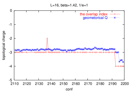
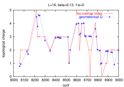
Figure 1: Comparison of the topological charge $Q$; the geometrical definition $Q=Z_{geo}Q_{geo}$ after “cooling”, and the index of the overlap-Dirac operator with $s=0.6$. The agreement is better for $1/\epsilon=1$ (left) than for $1/\epsilon=0$ (right).

3.3 Large negative mass Wilson fermion

Now let us discuss the lattice QCD with the determinant of Wilson fermion with negative mass at cut-off scale $-(1+s)/a$ as seen in Eq.(2.18). This is a more direct way to suppress the small eigenvalue of $H_{W}$, or keep topological charge, since the determinant $\det a^{2}H_{W}^{2}$ would give a very small Boltzmann weight if $H_{W}$ touches zero. For the gauge action, we use the topology conserving action Eq.(2.15) again with three values of $1/\epsilon$: 1, 2/3, and 0. We set the hopping parameter $\kappa_{hop}=1/(8-(1+s))=0.208$, which is known to be an optimal choice for the locality of the overlap Dirac operator [96], and the conventional pseudo-fermion method is performed in the hybrid Monte Carlo steps to calculate the fermion determinant. For thermalization, we performed more than 500 trajectories before measuring observables.

The topological charge is evaluated in the same way as explained in the previous subsection, namely, by the geometrical definition Eq.(3.16) after 100-200 of the quenched HMC steps with increasing $\beta$, switching off the Wilson fermion. Although the topological charge is expected to be more stable in this method, there may be a large scaling violation. Careful comparison with quenched studies without the determinant would be important.

The simulation parameters are summarized in Table. 1

3.4 Numerical implementation of the overlap Dirac operator

For the overlap Dirac operator, Eq.(2.1), we use the Wilson Dirac Hamiltonian $aH_{W}=\gamma_{5}(aD_{W}-1-s)$ with $s=0.6$, which is empirically known as an optimal choice to suppress the small eigen-modes of $|aH_{W}|$ at $1/a\sim$2.0GeV in quenched QCD. The sign function is approximated by the Chebyshev polynomial (See Fig. 2);

$$\mbox{sgn}_{\mathrm{Cheb}}(aH_{W})=aH_{W}/\mbox{sqrt}_{\mathrm{Cheb}}(a^{2}H_{W}^{2}),$$ (3.17)

where the function $\mbox{sqrt}_{\mathrm{Cheb}}(a^{2}H_{W}^{2})$ in the range [a,b] is written

$$1/\mbox{sqrt}_{\mathrm{Cheb}}(x) \equiv \sum_{i=0}^{N_{\mathrm{poly}}}c_{i}T_{i}(x^{\prime}),\;\;\;\;\;x^{\prime}=\frac{b+a}{b-a}-\frac{2}{b-a}x$$

$$c_{i} = \frac{2}{\pi}\int_{0}^{\pi}\frac{\sqrt{2}}{\sqrt{(b+a)-(b-a)\cos\phi}}\cos n\phi d\phi,$$

$$T_{i}(t) = \cos n\phi,\;\;\;\;\;t=\cos\phi.$$ (3.18)

Note that the Chebyshev basis $T_{i}(x)$ (of order $i$) satisfies the orthogonal relation

$$\int_{-1}^{1}\frac{dt}{\sqrt{1-t^{2}}}T_{i}(t)T_{j}(t)=\delta_{ij}.$$ (3.19)

We use the numerical package ARPACK [97], which implements the implicitly restarted Arnoldi method, to measure the lowest eigenvalue $a=\lambda_{\mathrm{min}}^{2}$ and the highest $b=\lambda_{\mathrm{max}}^{2}$. In some cases, we calculate the 10 lowest modes explicitly, project them out of $H_{W}$, and use the approximation Eq.(3.17) after the projection, in the range $[a_{11},b]$ where we use the 11th eigenvalue for the lower bound; $a_{11}=\lambda_{11}^{2}$.

In order to determine the order of the polynomial, $N_{\mathrm{poly}}$, it is important to note that the accuracy is expressed as a function of $N_{\mathrm{poly}}$ and the condition number $\kappa=\lambda_{\mathrm{max}}/\lambda_{\mathrm{min}}=\sqrt{b/a}$,

$$\frac{\langle v|(1-\mbox{sgn}_{\mathrm{Cheb}}^{2}(aH_{W}))^{2}|v\rangle}{\langle v|v\rangle}\sim A\exp(-BN_{\mathrm{poly}}/\kappa),$$ (3.20)

for a random vector $|v\rangle$, where the constants $A\sim 0.3$ and $B\sim 4.2$ are turned out to be independent of $\beta$, $\epsilon$ and the lattice size $L$, as seen in Fig. 3. Note that the lhs. of Eq.(3.20) is zero when the sign function is exact and the approximation breaks down when $1/\kappa=0$.

We also use ARPACK to calculate the eigenvalues of $P_{-}DP_{-}$ and $P_{+}DP_{+}$, where $P_{\pm}=(1\pm\gamma_{5})/2$. The index can be obtained from the number of zero-modes of chirally projected Dirac operators. To construct the non-zero mode, $|\lambda\rangle$, of $D$, the formula

$$|\lambda\rangle=\frac{D-\lambda^{*}}{\mbox{Im}\lambda}P_{+}|\lambda\rangle=\frac{D-\lambda^{*}}{\mbox{Im}\lambda}P_{-}|\lambda\rangle,$$ (3.21)

is useful.

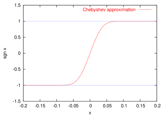
Figure 2: The Chebyshev approximation of sgn function. We set $N_{\mathrm{poly}}=60$ and the range $[a=0.1,b=1]$.

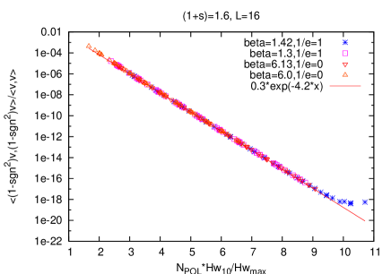
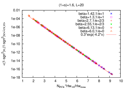
Figure 3: The accuracy Eq.(3.20) as a function of $N_{\mathrm{pol}}/\kappa$ on a 16⁴ lattice (left) and a 20⁴ lattice. We use 4 gauge configurations and 10 values of $N_{\mathrm{pol}}$ = 60–195 for each parameter set.

4 Wilson loops and the static quark potential

In order to confirm the practical feasibility of the topology conserving actions, Eq.(2.15) and Eq.(2.18), a careful comparison with the Wilson plaquette action should be done. In this section, we study gluonic quantities or Wilson loops to determine the lattice spacing, to estimate the scaling violations due to the change in the actions, and to test the perturbation theory with tadpole improved coupling. Then we can judge whether our naive expectation that $1/\epsilon$ effect is small (of order $O(a^{4})$) or the effect of the determinant, $\det H_{W}^{2}$, is negligible, is true or not.

4.1 The static quark potential

In the following, we assume that the topology of the gauge field does not affect the Wilson loops when the lattice size is large, say $L>1$ fm, and choose the run with $Q=0$ or $Q=1$ initial configuration for the measurement.

Wilson loops, $W(\vec{r},t)$’s, are measured using the smearing technique according to [98], where the spatial separation $\vec{r}/a$ is taken to be an integer multiples of vectors $\vec{v}=(1,0,0)$, $(1,1,0)$, $(2,1,0)$, $(1,1,1)$, $(2,1,1)$ and $(2,2,1)$. Assuming the Wilson loop is an exponential function

$$\langle W(\vec{r},t)\rangle=\exp(-V(\vec{r})t),$$ (4.1)

for large $t/a$, we extract the static quark potential $aV(\vec{r})$. The measurements are done every 20 trajectories and the errors are estimated by the jackknife method.

As a reference scale to determine the lattice spacing, we evaluate the Sommer scales $r_{0}$ and $r_{c}$ [99, 100] defined by $r_{0}^{2}F(r_{0})=1.65$ and $r_{c}^{2}F(r_{c})=0.65$, respectively. The force $F(r)$ on the lattice is given by a differentiation of the potential in the direction of $\vec{u}/a=(1,0,0)$;

$$a^{2}F(r_{I})=\frac{aV(\vec{r})-aV(\vec{r}-\vec{u})}{|\vec{u}/a|},$$ (4.2)

for $\vec{r}/|\vec{r}|=(1,0,0)$. $r_{I}$ is introduced to cancel $O(a)$ errors in the short distances at tree level,

$$\frac{1}{4\pi(r_{I}/a)^{2}} = -\frac{aG(\vec{r})-aG(\vec{r}-\vec{u})}{|\vec{u}/a|},$$

$$aG(\vec{r}) = \int^{\pi}_{-\pi}\frac{d^{3}k}{(2\pi)^{3}}\frac{\prod^{3}_{j=1}\cos(r_{j}k_{j}/a)}{4\sum_{j=1}^{3}\sin^{2}(k_{j}/2)}.$$ (4.3)

In Table 2 we present the values of the Sommer scales $r_{0}/a$, $r_{c}/a$, their ratio $r_{c}/r_{0}$, and the lattice spacing $a$ (We assume $r_{0}\sim 0.5$fm.). The data of $aV(\vec{r})$ and $r_{I}^{2}F(r_{I})$ in the case that $\vec{r}/a$ is an integer multiples of $\vec{u}/a$ are given in Tables 3, 4 and 5.

Lattice size	$1/\epsilon$	$\beta$	statistics	$r_{0}/a$	$r_{c}/a$	$r_{c}/r_{0}$	$a$
$12^{4}$	1	1.0	3800	3.257(30)	1.7081(50)	0.5244(52)	0.15fm
quenched		1.2	3800	4.555(73)	2.319(10)	0.5091(81)	0.11fm
		1.3	3800	5.140(50)	2.710(14)	0.5272(53)	0.1fm
	2/3	2.25	3800	3.498(24)	1.8304(60)	0.5233(41)	0.14fm
		2.4	3800	4.386(53)	2.254(10)	0.5141(61)	0.11fm
		2.55	3800	5.433(72)	2.809(18)	0.5170(67)	0.09fm
$16^{4}$	1	1.3	2300	5.240(96)	2.686(13)	0.5126(98)	0.1fm
quenched		1.42	2247	6.240(89)	3.270(26)	0.5241(83)	0.08fm
	2/3	2.55	1950	5.290(69)	2.738(15)	0.5174(72)	0.09fm
		2.7	2150	6.559(76)	3.382(22)	0.5156(65)	0.08fm
$14^{4}$	1	0.75	162	4.24(15)	2.240(37)	0.528(24)	0.12fm
with $\det H_{W}^{2}$	2/3	1.8	261	4.94(19)	2.361(26)	0.478(19)	0.10fm
	0	5.0	162	4.904(90)	2.691(42)	0.549(13)	0.10fm
$16^{4}$	1	0.8	207	4.81(17)	2.442(48)	0.508(20)	0.10fm
with $\det H_{W}^{2}$	2/3	1.75	189	4.71(19)	2.279(48)	0.484(22)	0.11fm
	0	5.2	225	7.09(17)	3.462(55)	0.489(13)	0.07fm
continuum limit [100]						0.5133(24)

Table 2: Sommer scales $r_{0}/a$, $r_{c}/a$ and their ratio. Here we assume $r_{0}\sim$0.5fm.

	$1/\epsilon=1$		124 quenched		164 quenched
$\beta$	$r/a$	$r_{I}/a$	$aV(\vec{r})$	$r_{I}^{2}F(r_{I})$	$aV(\vec{r})$	$r_{I}^{2}F(r_{I})$
1.0	1		0.50459(20)
	2	1.36	0.77828(61)	0.5056(10)
	3	2.28	0.9629(15)	0.9520(69)
	4	3.31	1.1176(27)	1.691(26)
	5	4.36	1.2623(45)	2.751(80)
	6	5.39	1.4052(77)	4.33(22)
1.2	1		0.44877(16)
	2	1.36	0.65982(39)	0.38993(65)
	3	2.28	0.78291(80)	0.6346(34)
	4	3.31	0.8775(13)	1.034(10)
	5	4.36	0.9588(29)	1.545(45)
	6	5.39	1.0322(47)	2.23(12)
1.3	1		0.42730(10)		0.42709(20)
	2	1.36	0.61711(34)	0.35252(99)	0.61710(66)	0.35099(68)
	3	2.28	0.72140(69)	0.53909(48)	0.72130(92)	0.5490(29)
	4	3.31	0.7977(12)	0.848(14)	0.7961(15)	0.8325(81)
	5	4.36	0.8608(21)	1.240(36)	0.8583(23)	1.180(32)
	6	5.39	0.9230(25)	1.887(85)	0.9150(27)	1.809(79)
	7	6.41			0.9636(51)	1.93(24)
	8	7.43			1.0215(51)	3.09(37)
1.42	1				0.40443(15)
	2	1.36			0.57416(43)	0.31444(58)
	3	2.28			0.66091(75)	0.4567(22)
	4	3.31			0.7200(12)	0.6583(61)
	5	4.36			0.7691(17)	0.940(14)
	6	5.39			0.8076(24)	1.189(48)
	7	6.41			0.8457(30)	1.675(64)
	8	7.43			0.8832(37)	1.91(14)

Table 3: Potential and force values in the case that $\vec{r}/a$ is an integer multiples of the unit vector $\vec{u}/a=(1,0,0)$. Results with $1/\epsilon$ = 1 (quenched).

	$1/\epsilon=2/3$		124 quenched		164 quenched
$\beta$	$r/a$	$r_{I}/a$	$aV(\vec{r})$	$r_{I}^{2}F(r_{I})$	$aV(\vec{r})$	$r_{I}^{2}F(r_{I})$
2.25	1		0.48470(15)
	2	1.36	0.74012(57)	0.47189(97)
	3	2.28	0.9077(13)	0.8640(56)
	4	3.31	1.0463(22)	1.515(21)
	5	4.36	1.1701(38)	2.353(64)
	6	5.39	1.2901(58)	3.64(15)
2.4	1		0.44908(12)
	2	1.36	0.66434(41)	0.39770(70)
	3	2.28	0.79152(84)	0.6557(37)
	4	3.31	0.8889(15)	1.065(12)
	5	4.36	0.9749(23)	1.635(32)
	6	5.39	1.0541(30)	2.401(74)
2.55	1		0.42013(11)		0.42042(16)
	2	1.36	0.60682(36)	0.34493(58)	0.60786(51)	0.34590(72)
	3	2.28	0.70826(72)	0.5230(28)	0.71227(95)	0.5337(32)
	4	3.31	0.7806(13)	0.7913(90)	0.7878(16)	0.8211(93)
	5	4.36	0.8430(18)	1.187(18)	0.8538(22)	1.210(21)
	6	5.39	0.8986(23)	1.686(37)	0.9157(29)	1.765(47)
	7	6.41			0.9710(43)	2.229(84)
	8	7.43			1.0266(52)	2.94(15)
2.7	1				0.39590(15)
	2	1.36			0.56100(44)	0.30650(53)
	3	2.28			0.64733(62)	0.4456(22)
	4	3.31			0.70527(90)	0.6329(56)
	5	4.36			0.7528(14)	0.907(14)
	6	5.39			0.7937(19)	1.309(28)
	7	6.41			0.8321(24)	1.531(44)
	8	7.43			0.8703(29)	2.035(80)

Table 4: Same as Table 3, but with $1/\epsilon$ = 2/3 (quenched).

$1/\epsilon=1$		144 $\det H_{W}^{2}$ $\beta=0.75$		164 $\det H_{W}^{2}$ $\beta=0.8$
$r/a$	$r_{I}/a$	$aV(\vec{r})$	$r_{I}^{2}F(r_{I})$	$aV(\vec{r})$	$r_{I}^{2}F(r_{I})$
1		0.50199(51)		0.48708(37)
2	1.36	0.7198(18)	0.4025(31)	0.6943(13)	0.3829(22)
3	2.28	0.8480(32)	0.661(14)	0.8137(25)	0.616(14)
4	3.31	0.9457(50)	1.068(49)	0.8936(42)	0.873(45)
5	4.36	1.037(55)	1.74(12)	0.9681(57)	1.416(87)
6	5.39	1.097(85)	1.83(26)	1.0334(85)	1.98(28)
7	6.41			1.110 (11)	3.01(37)
8	7.43			1.151(14)	2.26(80)
$1/\epsilon=2/3$		144 $\det H_{W}^{2}$ $\beta=1.8$		164 $\det H_{W}^{2}$ $\beta=1.75$
$r/a$	$r_{I}/a$	$aV(\vec{r})$	$r_{I}^{2}F(r_{I})$	$aV(\vec{r})$	$r_{I}^{2}F(r_{I})$
1		0.49349(42)		0.50630(46)
2	1.36	0.7125(15)	0.4046(25)	0.7363(18)	0.4249(31)
3	2.28	0.8323(25)	0.6178(91)	0.8605(35)	0.640(20)
4	3.31	0.9294(48)	1.062(40)	0.9680(68)	1.175(65)
5	4.36	1.0000(68)	1.34(12)	1.0423(88)	1.41(16)
6	5.39	1.0655(92)	1.99(24)	1.118(15)	2.30(39)
7	6.41			1.185(17)	2.64(55)
8	7.43			1.261(24)	4.1(1.2)
$1/\epsilon=0$		144 $\det H_{W}^{2}$ $\beta=5.0$		164 $\det H_{W}^{2}$ $\beta=5.2$
$r/a$	$r_{I}/a$	$aV(\vec{r})$	$r_{I}^{2}F(r_{I})$	$aV(\vec{r})$	$r_{I}^{2}F(r_{I})$
1		0.45795(42)		0.42080(26)
2	1.36	0.6547(12)	0.3634(19)	0.58846(72)	0.3098(13)
3	2.28	0.7606(22)	0.5466(84)	0.6722(12)	0.4318(48)
4	3.31	0.8369(32)	0.833(28)	0.7246(16)	0.617(14)
5	4.36	0.9000(51)	1.200(70)	0.7745(25)	0.872(43)
6	5.39	0.9730(75)	2.21(13)	0.8120(27)	1.137(60)
7	6.41			0.8426(37)	1.21(10)
8	7.43			0.8762(39)	1.84(15)

Table 5: Same as Table 3, with $\det H_{W}^{2}$.

$r_{c}/r_{0}$ is a good quantity to estimate the scaling violation, comparing with the value $r_{c}/r_{0}=0.5133(24)$ in the continuum limit, which was obtained with the plaquette action [100]. Fig. 5 shows the $a^{2}$ dependence of this ratio with different values of $1/\epsilon$. The quenched results with $1/\epsilon$ = 2/3 and 1 agree very well with Ref [100] except for the coarsest lattice points around $(a/r_{0})^{2}\simeq$ 0.1. Also in the case with $\det H_{W}^{2}$, as seen in Fig. 5, any large scaling violation has not been seen although the statistics are much poorer.

Fig. 7 presents the quark potential itself in a dimensionless combination, i.e. $\hat{V}(\vec{r})\equiv r_{0}(V(\vec{r})-V(r_{c}))$ as a function of $|\vec{r}|/r_{0}$. $V(r_{c})$ is evaluated by an interpolation of the data in the direction $\vec{r}/|\vec{r}|=(1,0,0)$. The data at $\beta$ =1.3, $1/\epsilon=1$ in the quenched case and at $\beta=0.75$, $1/\epsilon=1$ with $\det H_{W}^{2}$ are plotted together with the curve representing the continuum limit obtained in [100]. The agreement is satisfactory (less than two sigma) for long distances $|\vec{r}|/r_{0}>$ 0.5. For short distances, on the other hand, one can see deviations of order 10%, as shown in Fig. 7, where the ratio $(\hat{V}(\vec{r})-\hat{V}_{\mathrm{cont}}(|\vec{r}|))/\hat{V}_{\mathrm{cont}}(|\vec{r}|)$ is plotted. $\hat{V}_{\mathrm{cont}}(|\vec{r}|)$ represents the curve in the continuum limit drawn in Fig. 7. The plots at $\vec{r}/a$ = $(1,0,0)$ and $(2,0,0)$ obviously deviate from zero in the upward direction, while the plots at $(1,1,0)$ and $(1,1,1)$ are lower than zero. This fact indicates the rotational symmetry violation in a short distance. Let us concentrate on the point $(1,0,0)$ as a function of the lattice spacing, as seen in Fig. 8 (left panel). We find that the size of the violation is quite similar to that with Wilson plaquette action and independent of $1/\epsilon$. One might think that the rotational symmetry goes worse in the continuum limit, but one should note the fact that the relevant scale of the observable also diverges as $1/a$. After a correction at the tree level by introducing $d_{I}$ as $1/(4\pi d_{I})=G(d)$, which is an analogue of $r_{I}$ in Eq.(4.1) but is defined for the potential, we obtain the plot on the right panel of Fig. 8, where one can see an improvement. The remaining deviation should be of order $\alpha_{s}(1/a)$, which would vanish as $\sim 1/\ln(1/a)$ near the continuum limit. The data at $\vec{r}=(1,0,0)$ with $\det H_{W}^{2}$ have larger statistical errors but show a very similar behavior.

These observations show that both of scaling violations and rotational symmetry violations are reasonable and the topology conserving actions are feasible in the numerical studies.

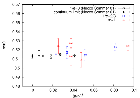
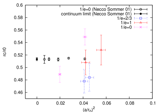
Figure 4: Quenched results (without $\det H_{W}^{2}$) of $r_{c}/r_{0}$. Squares and triangles are data for the topology conserving gauge action with $1/\epsilon$ = 2/3 and 1, respectively. Open circles represent the Wilson plaquette gauge action (from [100]) and the filled circle is their continuum limit.

Figure 5: The same as Fig.5 with $\det H_{W}^{2}$.

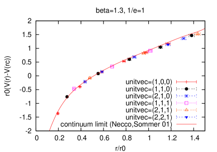
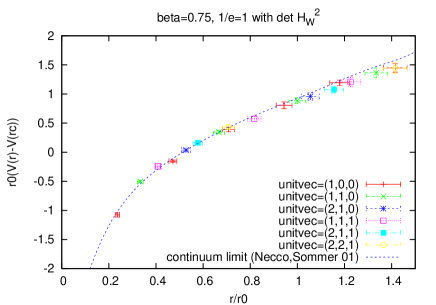
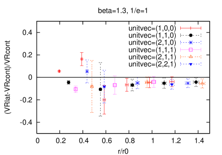
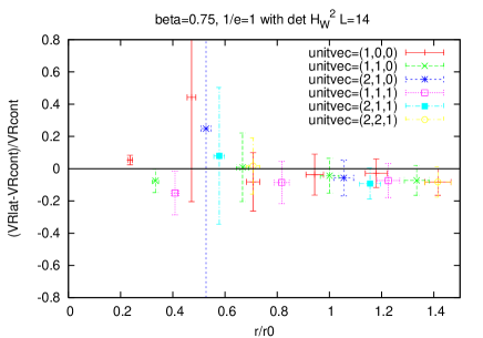
Figure 6: Static quark potential at $\beta=1.3$, $1/\epsilon$ = 1 (quenched) on a $12^{4}$ lattice (left) and $\beta=0.75$, $1/\epsilon$ = 1 (with $\det H_{W}^{2}$) on a $14^{4}$ lattice (right) . The curve is the continuum limit obtained by an interpolation of the data of [100]. Different symbols show $V(\vec{r})$’s with different orientations parallel to $\vec{v}$’s.

Figure 7: Violation of rotational symmetry $(\hat{V}(\vec{r})-\hat{V}_{\mathrm{cont}}(|\vec{r}|))/\hat{V}_{\mathrm{cont}}(|\vec{r}|)$, where $\hat{V}_{\mathrm{cont}}(|\vec{r}|)$ denotes the continuum limit. Results for $\beta$ = 1.3, $1/\epsilon$ = 1 (quenched) and $\beta$ = 0.75, $1/\epsilon$ = 1 (with $\det H_{W}^{2}$) are shown. The error of $\hat{V}_{\mathrm{cont}}(|\vec{r}|)$ is not taken into account ($<1$%).

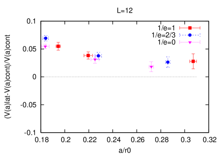
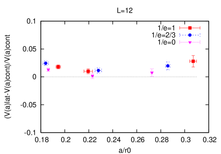
Figure 8: $(\hat{V}(\vec{r})-\hat{V}_{\mathrm{cont}}(|\vec{r}|))/\hat{V}_{\mathrm{cont}}(|\vec{r}|)$ for $\vec{r}=(1,0,0)$. Quenched results with different $\beta$ and $1/\epsilon$ values are plotted as a function of $a/r_{0}$. Left and right panels show the plot without and with the tree level improvement of the argument $\vec{r}$, respectively. See the text for details.

Finally, we confirm our assumption that the topology does not affect the quark potential by measuring $r_{0}$ for two initial value of $Q$ (0 and $-3$). Measurements are done on a $16^{4}$ lattice at $\beta$ = 1.42, $1/\epsilon$ = 1, for which the probability of the topology change is extremely small as discussed in Sec. 5. Our results are $r_{0}/a$ = 6.24(9) for the $Q=0$ initial condition and 6.11(13) for $Q=-3$. Details are seen in Table. 6.

Table 6: The quark potential with different initial topological charge. The results are at $1/\epsilon=1.0$ and $\beta=1.42$ on the $L=16$ lattice. Any large discrepancies are not seen.

$Q_{\mathrm{init}}$	$\Delta\tau$	$N_{mds}$	acceptance	StabQ	plaquette	$r_{0}/a$	$r_{c}/r_{0}$
0	0.01	20	82%	961	0.59167(1)	6.240(89)	0.5241(83)
-3	0.01	20	83%	514	0.59162(1)	6.11(13)	0.513(12)

4.2 Perturbative renormalization of the gauge coupling

From $1\times 1$ Wilson loop, $W(1,1)$, the so-called “mean field improved” bare gauge coupling can be defined. In quenched study with the standard Wilson plaquette action, it is known that the perturbation theory with mean field improvement coupling converges very well. Here we would like to define the mean field improved coupling with the topology conserving gauge action, Eq.(2.15), evaluate the coupling renormalization and see its convergence in 2-loop perturbation theory.

Two-loop corrections to the gauge coupling for general one-plaquette actions (constructed by the plaquette only and no rectangular term is involved.) is calculated by Ellis et al. [101]. Using their formula, the renormalized gauge couping $g_{M}$ defined in the “Manton” scheme is given by

$$\frac{1}{g_{M}^{2}}=\frac{1}{g^{2}}+A_{1}+A_{2}g^{2},$$ (4.4)

where $g$ denotes the bare coupling and the coefficients $A_{1}$ and $A_{2}$ are calculated as

$$A_{1} = s_{4}\frac{2N_{c}^{3}-3}{N_{c}}+t_{4}(N_{c}^{2}+1),$$

$$A_{2} = a_{R}[s_{4}(2N_{c}^{2}-3)+t_{4}N_{c}(N_{c}^{2}+1)]+s_{6}\frac{15(N_{c}^{4}-3N_{c}^{2}+3)}{8N_{c}^{2}}$$ (4.5)

$$+u_{6}\frac{3(2N_{c}^{2}-3)(N_{c}^{2}+3)}{8N_{c}}+t_{6}\frac{3}{8}(N_{c}^{2}+1)(N_{c}^{2}+3)$$

$$-s_{4}^{2}\frac{9N_{c}^{4}-30N_{c}^{2}+36}{2N_{c}^{2}}-2s_{4}t_{4}\frac{(2N_{c}^{2}-3)(N_{c}^{2}+2)}{N_{c}}-t_{4}^{2}(N_{c}^{2}+1)(N_{c}^{2}+2).$$

Here, the parameters are $N_{c}=3$, $s_{4}=-1/4!$, $s_{6}=1/6!$, $t_{4}=1/(4N_{c}\epsilon)$, $t_{6}=1/(8N_{c}^{2}\epsilon^{2})$, $u_{6}=-1/(4!N_{c}\epsilon)$, and $a_{R}=-0.0011(2)$. The values of the next-to-leading and next-to-next-to-leading order coefficients $A_{1}$ and $A_{2}$, when $1/\epsilon=1,2/3$ and 0, are given in Table 7.

Let us define the mean field improved coupling $\bar{g}^{2}$ by

$$\frac{1}{\bar{g}^{2}}=\frac{P}{g^{2}}\left(\frac{1}{1-(1-P)/\epsilon}+\frac{(1-P)/\epsilon}{(1-(1-P)/\epsilon)^{2}}\right),$$ (4.6)

with the measured value of the plaquette expectation value $P=\langle W(1,1)\rangle$ (see Table 1). It is defined from a coefficient of $F_{\mu\nu}^{2}$ when we rewrite $P_{\mu\nu}=P\exp(ia^{2}F_{\mu\nu})$ and expand the action Eq.(2.15)[102] .

A perturbative expectation value of the plaquette, or $1\times 1$ Wilson loop, is evaluated with the general one-plaquette action by Heller et al. [103] as

$$\langle W(1,1)\rangle = 1-g^{2}\frac{(N_{c}^{2}-1)}{N_{c}}\bar{W}_{2}(1,1)-g^{4}(N_{c}^{2}-1)X(1,1)$$ (4.7)

$$+g^{4}\frac{(2N_{c}^{2}-3)(N_{c}^{2}-1)}{6N_{c}^{2}}\bar{W}_{2}(1,1)^{2}-g^{4}\frac{(N_{c}^{2}-1)}{6N_{c}}CZ(1,1).$$

Here $\bar{W}_{2}(1,1)$ and $X(1,1)$ are from the original calculation [104] for the Wilson plaquette gauge action, and $Z(1,1)=(1-1/V)\bar{W}_{2}(1,1)/4$ (on a symmetric lattice $V=L^{4}$) is introduced for generalization. Their values are $\bar{W}_{2}(1,1)=1/8$, $X(1,1)=-1.01\times 10^{-4}$ and $Z(1,1)=1/32$ in the infinite volume limit. The constant $C$ is written

$$C=\left[\sum_{R}6g^{2}\frac{s_{R}(\beta)T(R)C_{2}(R)}{d_{R}}-N_{c}\right],$$ (4.8)

where $C_{2}(R)$ denotes the quadratic Casimir operator in a representation $R$ of the group $SU(N_{c})$. $d_{R}$ is the dimension of the representation $R$, and $T(R)$ is defined such that $\mbox{Tr}_{R}(t^{a}t^{b})=T(R)\delta^{ab}$ for the group generator $t^{a}$. The coupling $s_{R}(\beta)$ is defined as a coupling when we rewrite the gauge action in terms of a general form of the one-plaquette action,

$$S_{G}=\sum_{x,\mu,\nu}\sum_{R}s_{R}(\beta)\left[1-\frac{1}{d_{R}}\mbox{Re}\mbox{Tr}_{R}P^{R}_{\mu\nu}(x)\right],$$ (4.9)

where $P_{\mu\nu}^{R}$ denotes the plaquette variable in the $R$ representation. The values of these parameters for the topology conserving gauge action Eq.(2.15) are

$$s_{3}(\beta)=\left(1+\frac{11}{6\epsilon}\right)\beta,\;\;\;s_{6}(\beta)=-\frac{1}{3\epsilon}\beta,\;\;\;s_{8}(\beta)=-\frac{4}{9\epsilon}\beta,$$ (4.10)

The other parameters are $T(3)=1/2$, $T(6)=5/2$, $T(8)=3$, $C_{2}(3)=4/3$, $C_{2}(6)=10/3$ and $C_{2}(8)=3$. With these numbers, we obtain $C=5-20/\epsilon$ and we finally get

$$\langle W(1,1)\rangle=1-\frac{g^{2}}{3}+\left(\frac{5}{18\epsilon}-\frac{5}{144}\right)g^{4}.$$ (4.11)

Since the perturbative relation between the bare coupling $g$ and the boosted coupling $\bar{g}$ Eq.(4.6) is given by

$$\frac{1}{\bar{g}^{2}}=\frac{1}{g^{2}}+B_{1}+B_{2}g^{2},$$ (4.12)

where

$$B_{1}=-\frac{1}{3}\left(1-\frac{2}{\epsilon}\right),\;\;\;B_{2}=\left(1-\frac{2}{\epsilon}\right)\left(\frac{5}{18\epsilon}-\frac{5}{144}\right)-\frac{2}{9\epsilon}+\frac{1}{3\epsilon^{2}},$$ (4.13)

one obtains the Manton coupling in terms of the boosted coupling as

$$\frac{1}{g_{M}^{2}}=\frac{1}{\bar{g}^{2}}+(A_{1}-B_{1})+(A_{2}-B_{2})\bar{g}^{2}.$$ (4.14)

Numerical values of $B_{i}$ and $A_{i}-B_{i}$ are listed in Table 7. One can see the effect of the mean field improvement; the two-loop coefficient $A_{2}$ is significantly reduced by reorganizing the perturbative expansion as in Eq.(4.14).

$1/\epsilon$	$A_{1}$	$A_{2}$	$B_{1}$	$B_{2}$	$A_{1}-B_{1}$	$A_{2}-B_{2}$
0	$-$0.20833	$-$0.03056	$-$0.33333	$-$0.03472	0.12500	0.00416
2/3	0.34722	$-$0.04783	0.11111	$-$0.05015	0.23611	0.00233
1	0.62500	$-$0.10276	0.33333	$-$0.13194	0.29167	0.02919

Table 7: Next-to-leading and next-to-next-to-leading order coefficients of the coupling renormalization for various $\epsilon$. Mean field improved coefficients $A_{1}-B_{1}$, $A_{2}-B_{2}$ are also presented. See the text for details.

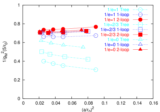
Figure 9: $1/g_{M}^{2}$ in the Manton scheme are plotted. The mean field improved expression Eq.(4.14) is used with the measured plaquette expectation value. Different symbols distinguish the value of $1/\epsilon$ (1 for circles, 2/3 for squares, 0 for triangles). Open symbols with dot-dashed line represent tree-level results and open symbols with dashed lines are one-loop. The best results including two-loop corrections are shown by filled symbols with solid lines.

With these results, the Manton coupling is obtained for each lattice parameters. In Fig. 9, we plot the coupling evaluated at a reference scale $5/r_{0}$ as a function of $a^{2}/r_{0}^{2}$. We use the two-loop renormalization equation to run $g_{M}$ to the reference scale. Although $g_{M}$ is very different at the tree level, the one-loop results are already in good agreement among the different values of $1/\epsilon$. The two-loop corrections show that the perturbative expansion converges very well and a good agreement among different $1/\epsilon$. Moreover, the scaling toward the continuum limit seems also good in the two-loop level plots.

5 Stability of the topological charge

5.1 Admissibility condition and topology stability

As discussed in Sec.2, it is difficult to construct an exact and practical geometrical definition of the topological charge for non-Abelian theories, unless the gauge fields are very smooth [105] (note that (3.16) gives non-integers). But even if we choose larger $\epsilon\gg 1/20$, it is quite possible that the barriers among the topological sectors are high enough to suppress topology changes for hundreds of HMC trajectories, since any gauge action has a tendency to prevent the topology transitions in the continuum limit.

In Table. 8 we present our data of the topological charge stability,

$$\mbox{Stab}_{Q}\equiv\frac{N_{\mathrm{trj}}}{\tau_{\mathrm{plaq}}\times\#Q},$$ (5.1)

where $\tau_{\mathrm{plaq}}$ is the plaquette autocorrelation time, which is measured according to Appendix E of [106]. $N_{\mathrm{trj}}$ denotes the total length of the HMC trajectories and $\#Q$ is the number of topology changes during the trajectories. This definition, $\mbox{Stab}_{Q}$, gives a mean number of uncorrelated gauge configurations which can be sampled without changing the topology along the simulations. But we should mention that it only gives an upper limit, because the topological charge is measured only once per 10–20 trajectories and we may underestimate the topology changes if $Q$ jumps and returns quickly to the original value within this interval. Therefore, $\mbox{Stab}_{Q}$ is not reliable when the topology change is very frequent.

Lattice	$1/\epsilon$	$\beta$	$r_{0}/a$	$N_{\mathrm{trj}}$	$\tau_{\mathrm{plaq}}$	$\#Q$	StabQ
$12^{4}$	1	1.0	3.257(30)	18000	2.91(33)	696	9
quenched		1.2	4.555(73)	18000	1.59(15)	265	43
		1.3	5.140(50)	18000	1.091(70)	69	239
	2/3	2.25	3.498(24)	18000	5.35(79)	673	5
		2.4	4.386(53)	18000	2.62(23)	400	17
		2.55	5.433(72)	18000	2.86(33)	123	51
	0	5.8	[3.668(12)]	18205	30.2(6.6)	728	1
		5.9	[4.483(17)]	27116	13.2(1.5)	761	3
		6.0	[5.368(22)]	27188	15.7(3.0)	304	6
$16^{4}$	1	1.3	5.240(96)	11600	3.2(6)	78	46
quenched		1.42	6.240(89)	5000	2.6(4)	2	961
	2/3	2.55	5.290(69)	12000	6.4(5)	107	18
		2.7	6.559(76)	14000	3.1(3)	6	752
	0	6.0	[5.368(22)]	3500	11.7(3.9)	14	21
		6.13	[6.642(–)]	5500	12.4(3.3)	22	20
$20^{4}$	1	1.3	—	1240	2.6(5)	14	34
quenched		1.42	—	7000	3.8(8)	29	64
	2/3	2.55	—	1240	3.4(7)	15	24
		2.7	—	7800	3.5(6)	20	111
	0	6.0	—	1600	14.4(7.8)	37	3
		6.13	—	1298	9.3(2.8)	4	35
$14^{4}$	1	0.75	4.24(15)	3500	5.05(82)	0	$>$693
with $\det H_{W}^{2}$	2/3	1.8	4.94(19)	5370	11.1(2.1)	0	$>$483
	0	5.0	4.904(90)	3120	21.4(6.5)	0	$>$146
$16^{4}$	1	0.8	4.81(17)	627	0.69(10)	0	$>$908
with $\det H_{W}^{2}$	2/3	1.75	4.71(19)	580	1.64(40)	0	$>$353
	0	5.2	7.09(17)	730	1.54(27)	0	$>$474

Table 8: The stability of the topological charge, $\mbox{Stab}_{Q}$. The HMC trajectory length $N_{\mathrm{trj}}$, the plaquette autocorrelation time $\tau_{\mathrm{plaq}}$, and the number of topology change $\#Q$ are also summarized.

In Fig. 10 the results are plotted as a function of the lattice spacing squared. Clearly, one can see that the stability goes better as $1/\epsilon$ increases when the lattice spacing is the same. Also, the stability gets worse as the lattice size is increased from $L/a=12$ to $L/a=20$. This is no surprising, because the topology change occurs through local dislocations of gauge field and its probability scales as the volume. An important notice here is that the topological charge can be very stable in any case in the continuum limit. The stability quickly rises as $a\to 0$.

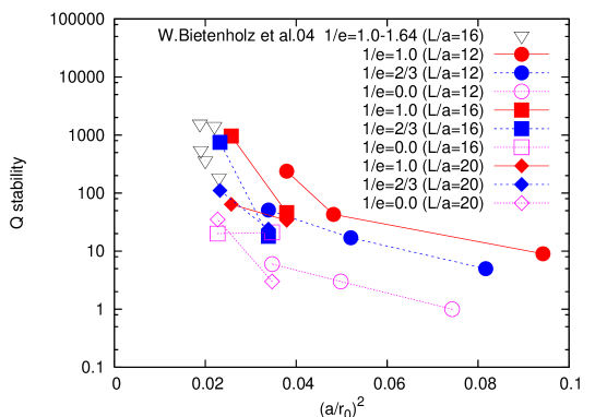
Figure 10: Stability of the topological charge in the quenched study. The results of different lattice size are plotted with different symbols; $L/a$ = 12 (circles), 16 (squares), 20 (upward triangles). The value of $1/\epsilon$ is distinguished by the line type: $1/\epsilon$ = 0 (dotted), 2/3 (dashed), 1 (solid). Downward triangles are the data of [34] measured on a 16⁴ lattice.

To study QCD in the $\epsilon$-regime in a fixed topological sector, the lattices $(1/\epsilon,\beta,L)\sim(1,1.42,16)$ and $(2/3,2.7,16)$ would be appropriate. Their physical size is around $L\sim$ 1.25 fm and the topological charge is stable for $(100-1000)\tau_{\mathrm{plaq}}$ trajectories.

5.2 Negative mass Wilson fermion to fix topology

In contrast to the case with topology conserving gauge action Eq.(2.15), one expects that the fermion determinant, $\det H_{W}^{2}$, can rigorously fix the topology of gauge fields along the simulation. In fact, as Table. 8 shows, the topology change has never occurred in every run with different parameters, which are chosen such that the lattice spacing is around $a\sim 0.08$–0.1fm. Our data show that $Q$ is unchanged for, at least, 100-1000 $\tau_{\mathrm{plaq}}$ trajectories, even if one ignores the thermalization steps.

6 The effects on the overlap Dirac operator

6.1 Low-lying mode distribution of $H_{W}$

As explained in Sec 3.4, the order of Chebyshev polynomial approximation, $N_{\mathrm{poly}}$ has to be proportional to the condition number, $\kappa=\lambda_{\mathrm{max}}/\lambda_{\mathrm{min}}$, in order to keep a certain desired accuracy. Since both topology conserving actions, Eq.(2.15) and Eq.(2.18) would play a role to suppress the occurrence of low-lying eigenvalues of $|aH_{W}|=|\gamma_{5}(aD_{W}-1-s)|$, they may be useful to reduce the numerical cost of calculating the overlap Dirac operator.

Fig. 11 shows a typical comparison of the eigenvalue distribution on a 16⁴ lattice. The values of $\beta$ and $\epsilon$ are chosen such that the Sommer scale $r_{0}/a$ is roughly equal to 5 (left panel) and 6.5-7 (right panel) , which correspond to $a\simeq 0.1$ fm and $a\simeq 0.08$ fm respectively. From the plot we observe that the density of the low-lying modes is relatively small for larger values of $1/\epsilon$ in quenched case. Let us discuss this more quantitatively. In Table 9 we list the probability, $P_{\lambda_{\mathrm{min}}<0.1}$, that a configuration has the lowest eigenvalue lower than 0.1. For the above example (left panel), the probability is 74% for the standard Wilson gauge action ($\beta=6.0$, $1/\epsilon$ = 0 quenched ), but it decreases to 53% (47%) for $1/\epsilon$ = 2/3 (1)(quenched). It is interesting to note that the data with $\det H_{W}^{2}$ show that the average of $\lambda_{\mathrm{min}}$ is not so large, but the occurrence of very small eigenvalues $\ll$0.1 is strongly suppressed. The lowest eigenvalue in these configurations is 1.2e-03 in the quenched case at $\beta=6.0$ and $1/\epsilon=0$, while it is 0.042 in the case with $\det H_{W}^{2}$ at $\beta=0.8$ and $1/\epsilon=1$.

Also, for another lattice spacing ($r_{0}/a\simeq$ 6.5) and lattice size $20^{4}$, a similar trend can be seen. In Table 9 we also present the ensemble average of the lowest eigenvalue $\lambda_{\mathrm{min}}$ and the inverse of condition numbers $\lambda_{\mathrm{max}}/\lambda_{\mathrm{min}}$ and $\lambda_{\mathrm{max}}/\lambda_{\mathrm{10}}$, where $\lambda_{\mathrm{10}}$ and $\lambda_{\mathrm{max}}$ denote the 10th and the highest eigenvalues respectively. We may conclude that the lowest eigenvalue is higher in average when we use the topology conserving actions. In the numerical implementation of the overlap-Dirac operator, the low-lying eigen-modes of $aH_{W}$ are often subtracted and treated exactly. Then the higher mode contributions are approximated by some polynomial or rational functions. Here, we assume that 10 lowest eigen-modes are subtracted and compare the relative numerical cost on the gauge configurations with different values of $1/\epsilon$. From Table 9 we observe that the reduced condition number is about a factor 1.2–1.4 smaller for $1/\epsilon$ = 1 than that for the standard Wilson gauge action.

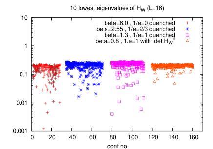
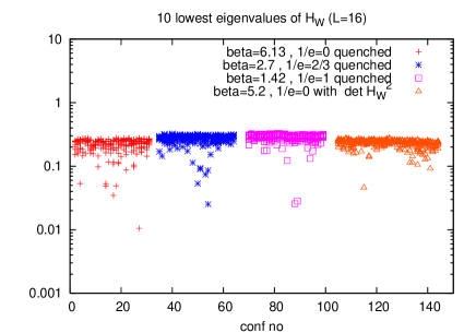
Figure 11: Ten lowest eigenvalues of $|aH_{W}|=|\gamma_{5}(aD_{W}-1.6)|$ for gauge configurations with $r_{0}/a\simeq 5$ (left) and $r_{0}/a\simeq 6.5$-7 (right). Quenched data are shown for $1/\epsilon$ = 1 (pluses), 2/3 (stars), 0 (squares) and triangles are the result with $\det H_{W}^{2}$. The lattice size is 16⁴.

lattice size	$1/\epsilon$	$\beta$	$r_{0}/a$	$P_{\lambda_{\mathrm{min}}<0.1}$	$\lambda_{\mathrm{min}}$	$\lambda_{\mathrm{min}}/\lambda_{\mathrm{max}}$	$\lambda_{\mathrm{10}}/\lambda_{\mathrm{max}}$
$20^{4}$	1	1.3	5.240(96)	0.64	0.0882(84)	0.0148(14)	0.03970(29)
quenched	2/3	2.55	5.290(69)	0.75	0.0604(53)	0.0101(08)	0.03651(27)
	0	6.0	[5.368(22)]	0.97	0.0315(57)	0.0059(34)	0.02766(46)
	1	1.42	6.240(89)	0.22	0.168(13)	0.0282(21)	0.04765(32)
	2/3	2.7	6.559(76)	0.19	0.151(11)	0.0251(19)	0.04646(37)
	0	6.13	[6.642(–)]	0.45	0.0861(83)	0.0126(15)	0.03775(50)
$16^{4}$	1	1.3	5.240(96)	0.47	0.111(12)	0.0187(21)	0.04455(31)
quenched	2/3	2.55	5.290(69)	0.53	0.1038(98)	0.0174(16)	0.04239(36)
	0	6.0	[5.368(22)]	0.74	0.0692(90)	0.0116(15)	0.03451(62)
	1	1.42	6.240(89)	0.07	0.219(13)	0.0367(21)	0.05233(26)
	2/3	2.7	6.559(76)	0.13	0.191(12)	0.0320(19)	0.05117(29)
	0	6.13	[6.642(–)]	0.27	0.139(10)	0.0232(17)	0.04384(38)
$16^{4}$	1	0.8	4.81(17)	0.12	0.1502(87)	0.0255(11)
with $\det H_{W}^{2}$	2/3	1.75	4.71(19)	0.55	0.0999(44)	0.0170(10)
	0	5.2	7.09(17)	0.05	0.1771(69)	0.0297(12)

Table 9: The probability, $P_{\lambda_{\mathrm{min}}<0.1}$, to sample a configuration such that $\lambda_{\mathrm{min}}<0.1$ where $\lambda_{\mathrm{min}}$ is the lowest eigenvalue of the hermitian Wilson-Dirac operator $|aH_{W}|=|\gamma_{5}(aD_{W}-1.6)|$. Averages of the lowest eigenvalue and the inverse of condition numbers are also listed. The Sommer scale $r_{0}/a$ is the results from $L=16$ lattice simulations. The values with [$\cdots$] are from [100] with an interpolation in $\beta$.

We also check that the above observation does not change when one shifts the value of $s$ in a reasonable range. In Fig. 12, a typical distributions of the low-lying eigen-modes for $s$ = 0.2–0.7 are plotted. We find that the advantage of the topology conserving actions does not change. Also, from these plots we can see that $s\sim 0.6$ is nearly optimal for all the cases.

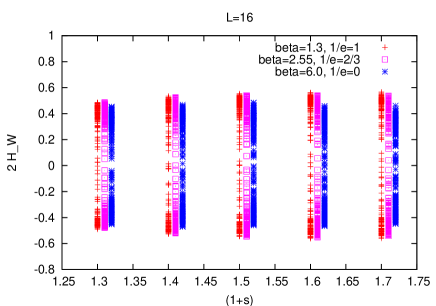
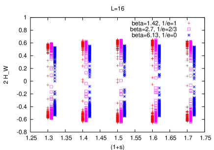
Figure 12: Ten near-zero eigenvalues on $16^{4}$ lattices with $r_{0}/a\sim 5.3$ (left) and $r_{0}/a\sim 6.5$ (right). Results are plotted as a function of $1+s$. Plots for $1/\epsilon$ = 2/3 and 0 are slightly shifted for clarity.

6.2 Locality

When we talk about the locality of the overlap-Dirac operator, it means that the norm $||D(x,y)v(y)||$ with a point source vector $v$ at $x_{0}$ should decay exponentially as a function of $|x-x_{0}|$ [29]

$$||D(x,y)v(y)||\sim C\exp(-D|x-x_{0}|),$$ (6.1)

where $C$ and $D$ are constants. Actually we observe this property, as seen in Fig. 13. The plot shows the results for different values of $1/\epsilon$ at the lattice scales $r_{0}/a\simeq$ 5.3 (left) and 6.5 (right). We find no remarkable difference on the locality when we change $1/\epsilon$.

Recently, it has been indicated that the mobility edge is more crucial quantity which governs the locality of the overlap-Dirac operator [69, 70, 71, 72, 73]. It would be interesting and important to see the dependence of the mobility edge on the parameters in the topology conserving actions, which should be done in the future works.

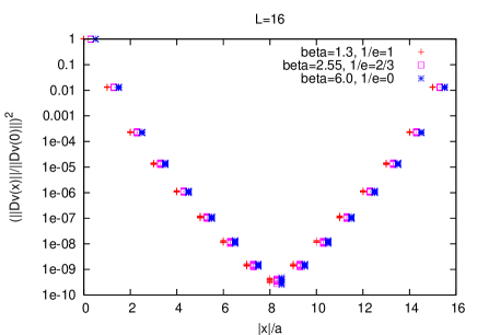
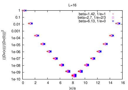
Figure 13: $(||D(x,y)v(y)||/||D(0,y)v(y)||)^{2}$ with $x_{0}=0$ measured on 10 gauge configurations for different values of $1/\epsilon$ (quenched). The lattice scale is $r_{0}/a\simeq 5.3$ (left) and 6.5 (right).

7 Lattice QCD in the $\epsilon$-regime with fixed $Q$

In previous sections we have discussed the topology conserving actions which might be helpful to the full QCD simulation with the overlap fermion determinant. Here we would like to show great uses of the overlap Dirac operator itself to measure physical observables. Once a set of configurations of $N_{f}=2$ or 3 full QCD is generated, it would be much easier and more reliable to extract physical quantities such as pion mass, decay constants, Kaon bag parameters, and so on, using the overlap Dirac operator which respects the “exact” chiral symmetry. One of attractive numerical applications would be the so-called $\epsilon$-regime, where both of chiral symmetry and topology have significant effects on the observables.

In this section we demonstrate the analysis of quenched lattice QCD in the $\epsilon$-regime to determine the low energy constants of the quenched chiral perturbation theory (qChPT). Of course, both quenched QCD and qChPT are unphysical and the data of pion decay constant or the chiral condensate have little relation to the true value of them in nature. However, this quenched study is still interesting to see how these low-energy constants can be extracted when the full QCD simulation is established in the future.

7.1 Meson correlators in the $\epsilon$-regime

It is believed that the low energy limit of QCD is described by the pion effective theory, or (q)ChPT. To determine the fundamental parameters of (q)ChPT is one of relevant issues of lattice QCD. In the so-called $\epsilon$-regime [43, 44, 45, 46, 47, 48], where the size of the space-time box is smaller than the pion Compton wave length; $L\ll 1/m_{\pi}$ (but larger than the QCD scale $1/\Lambda_{\mathrm{QCD}}\ll L$, which should be guaranteed so that the pion can be treated as a point particle and other heavier hadrons are decoupled.), (q)ChPT with a expansion parameter $\epsilon^{2}\sim m_{\pi}/\Lambda\sim p_{\pi}^{2}/\Lambda^{2}$, is still applicable. Here $\Lambda$ is a cutoff scale of the chiral Lagrangian roughly around 1 GeV. An important notice is that the low energy constants in (q)ChPT are defined at the cutoff scale and it does not depend on whether the system is in the $\epsilon$-regime or the large volume regime. Therefore, once $F_{\pi}$ or $\Sigma$ are determined in the $\epsilon$-regime, one can use them in the standard (q)ChPT in a larger volume. Analytic calculations of meson correlation functions in the $\epsilon$-regime have been widely studied for both ChPT and qChPT [107, 108, 109].

In the quenched case, the fundamental parameters of the effective theory are the pion decay constant, $F_{\pi}$, the chiral condensate, $\Sigma$, the singlet mass, $m_{0}$, and the coefficient of an additional singlet kinetic term, $\alpha$. Here we just present some results of 1-loop calculation, which are relevant to our numerical study. The details of calculation and the definition of the functions and coefficients are summarized in Appendix C. The scalar condensate at 1-loop level in $Q$ topological sector is given by

$$-\langle\bar{\psi}\psi\rangle=\Sigma_{Q}(\mu^{\prime})=\Sigma_{\mathrm{eff}}\mu^{\prime}(I_{|Q|}(\mu^{\prime})K_{|Q|}(\mu^{\prime})+I_{|Q|+1}(\mu^{\prime})K_{|Q|-1}(\mu^{\prime}))+\Sigma_{\mathrm{eff}}\frac{|Q|}{\mu^{\prime}}.$$ (7.1)

The triplet axial vector, scalar and pseudo-scalar correlators are given by

$$\langle A^{a}_{0}(x)A^{a}_{0}(0)\rangle_{Q} = -\frac{F_{\pi}}{V}-2m\Sigma_{Q}(\mu)\bar{\Delta}(x),$$ (7.2)

$$\langle S^{a}(x)S^{a}(0)\rangle_{Q} = C_{S}^{a}+\frac{\Sigma^{2}}{2F_{\pi}^{2}}\left[\frac{c_{-}}{N_{c}}(m_{0}^{2}\bar{G}(x)+\alpha\bar{\Delta}(x))-\bar{\Delta}(x)b_{-}\right],$$ (7.3)

$$\langle P^{a}(x)P^{a}(0)\rangle_{Q} = C_{P}^{a}-\frac{\Sigma^{2}}{2F_{\pi}^{2}}\left[\frac{c_{+}}{N_{c}}(m_{0}^{2}\bar{G}(x)+\alpha\bar{\Delta}(x))-\bar{\Delta}(x)b+\right].$$ (7.4)

The singlet scalar and pseudo-scalar correlators are

$$\langle S^{0}(x)S^{0}(0)\rangle_{Q} = C_{S}^{0}+\frac{\Sigma^{2}}{2F_{\pi}^{2}}\left[\frac{a_{-}}{N_{c}}(m_{0}^{2}\bar{G}(x)+\alpha\bar{\Delta}(x))-\bar{\Delta}(x)\frac{a_{+}+a_{-}-4}{2}\right],$$ (7.5)

$$\langle P^{0}(x)P^{0}(0)\rangle_{Q} = C_{P}^{0}-\frac{\Sigma^{2}}{2F_{\pi}^{2}}\left[\frac{a_{+}}{N_{c}}(m_{0}^{2}\bar{G}(x)+\alpha\bar{\Delta}(x))-\bar{\Delta}(x)\frac{a_{+}+a_{-}+4}{2}\right].$$ (7.6)

As mentioned in Appendix C, the results are valid only when $|Q|$ is small, which is a particular restriction of quenching the fermion determinant.

As these equations of qChPT show, the meson correlators in the $\epsilon$-regime should be quite sensitive to the topological charge and the fermion mass. These prominent $m$ and $Q$ dependences are used to evaluate the low energy constants, or namely, we fit our lattice data with the above equations, in which $F_{\pi}$, $\Sigma$, $m_{0}$ and $\alpha$ are treated as free parameters. The parameter $\Sigma$ always appears associated with the quark mass $m$ as $m\Sigma$ is renormalization scale and scheme independent. The value of $\Sigma$ in the following analysis should be understood as a bare quantity in the lattice regularization at a scale $1/a$. To relate them with the conventional scheme such as the $\overline{\mbox{MS}}$ scheme requires perturbative or non-perturbative matching, which is beyond the scope of this work.

7.2 Lattice observables with the exact chiral symmetry

We generate gauge link variables at $\beta=5.85$ and $1/\epsilon=0$ in the quenched approximation on a $L^{3}T=10^{3}\times 20$ lattice. The spacial length $L$ of the box is about 1.23 fm. We employ the massive Dirac operator for the valence quark,

$$D_{m}=\left(1-\frac{\bar{a}m}{2}\right)D+m,$$ (7.7)

where the bare quark mass are chosen to be very small; $am=$0.0016, 0.0032, 0.0048, 0.0064, 0.008, which corresponds 2.6–13MeV. The number of configurations for each topological sector is given in Table 10. We analyze the gauge configurations in $|Q|\leq 3$ sectors.

When the exact inversion of the overlap-Dirac operator is needed, we use the techniques described in Ref. [53]; for a given source vector $\eta$, we solve the equation

$$D_{m}\psi=\eta,$$ (7.8)

by separating the left and right handed components as $\psi=P_{-}\psi+P_{+}\psi$ and solving two equations

$$P_{-}\psi = (P_{-}D^{\dagger}_{m}D_{m}P_{-})^{-1}P_{-}D^{\dagger}_{m}\eta,$$ (7.9)

$$P_{+}\psi = (P_{+}D_{m}P_{+})^{-1}(P_{+}\eta-P_{+}D_{m}P_{-}\psi),$$ (7.10)

consecutively. (The above equations apply to positive $Q$ cases and the same procedure applies with a replacement $P_{+}\leftrightarrow P_{-}$ to negative $Q$ cases.) The conjugate gradient (CG) algorithm is used to invert the chirally projected matrices with the low-mode preconditioning in which 20 lowest eigen-modes are subtracted.

As one of special features of finite volume regime, a remarkable low-mode dominance in the chiral limit is expected [110, 111, 112] . Using ARPACK [97] again, we calculate 200 + $|Q|$ lowest mode eigenvalues and their eigenfunctions of the overlap Dirac operator. The index $Q$ is calculated at the same time. Note that these eigenvalues cover more than 15% of the circle in the complex space of the eigenvalues of $\bar{a}D$ as Fig. 14 shows. Then, the inverse of the overlap operator is decomposed as

$$D^{-1}_{m}(x,y)=\sum_{i=1}^{N_{\mathrm{low}}}\frac{1}{(1-\bar{a}m/2)\lambda_{i}+m}v_{i}(x)v_{i}^{\dagger}(y)+\Delta D_{m}^{-1}(x,y),$$ (7.11)

where $\lambda_{i}$’s are eigenvalues of $D$ and $v_{i}(x)$’s are their eigenvectors. We set $N_{\mathrm{low}}=200+|Q|$. In the following analysis, we often use the low-mode approximation of the expectation value (We will denote $\langle\cdots\rangle_{\mathrm{low}}$ instead of a simple bracket.) by inserting the low-mode part only,

$$D^{-1}_{m}(x,y)_{\mathrm{low}}=\sum_{i=1}^{N_{\mathrm{low}}}\frac{1}{(1-\bar{a}m/2)\lambda_{i}+m}v_{i}(x)v_{i}^{\dagger}(y),$$ (7.12)

to the propagators. This would be valid only when it is proved that the higher mode’s contributions are sufficiently small or can be canceled in the combination of different operators. An great advantage of using $D^{-1}_{m}(x,y)_{\mathrm{low}}$ instead of exact $D^{-1}_{m}(x,y)$ is that the inversion at any $x$ and $y$ is obtained without performing the CG algorithm, so that one can easily average the correlators over the space-time arguments, like

$$\left\langle\sum_{\vec{x}}\bar{\psi}\Gamma_{i}\psi(\vec{x},t)\bar{\psi}\Gamma_{i}\psi(\vec{0},0)\right\rangle^{Q}_{\mathrm{low}}\to\frac{1}{TL^{3}}\sum_{\vec{x}_{0},t_{0}}\left\langle\sum_{\vec{x}}\bar{\psi}\Gamma_{i}\psi(\vec{x},t+t_{0})\bar{\psi}\Gamma_{i}\psi(\vec{x}_{0},t_{0})\right\rangle^{Q}_{\mathrm{low}},$$ (7.13)

where $\Gamma_{i}$ denotes some gamma matrix. This so-called low-mode averaging dramatically reduces the fluctuation of the correlators as shown in Fig. 15, which is also reported in Refs. [113, 57].

Table 10: Number of configurations in each topological sector.

$|Q|$	0	1	2	3
# of confs.	20	45	44	24

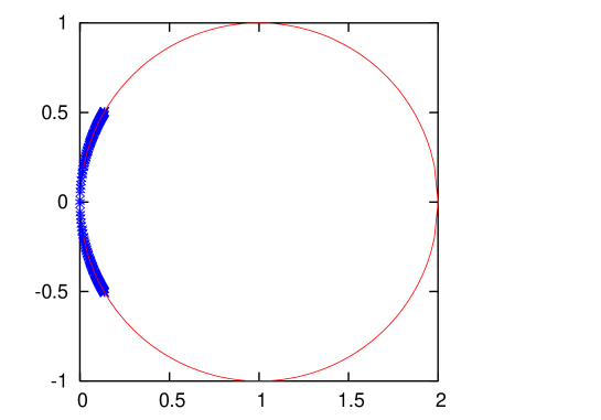
Figure 14: Lowest 202 eigenvalues of the overlap-Dirac operator $\bar{a}D$ at beta=5.85 on a $10^{3}20$ lattice with topological charge $Q=-2$. The eigenvalues cover a $\pi/3$ arc of the circle.

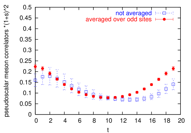
Figure 15: The pseudo-scalar correlator at $am=0.008$ and $|Q|=1$. Filled symbols denote the data with the low-mode averaging, where we use $(L/2)^{3}\times T/2$ source points, while open symbols are not averaged.

7.3 Numerical results

7.3.1 $F_{\pi}$ from the axial-vector correlator

First let us consider the axial-vector current correlator (7.2), which is most sensitive to $F_{\pi}$ and not contaminated by the parameters $m_{0}$ and $\alpha$. Here we do not use the low-mode approximation because 200+$|Q|$ modes are not sufficient to estimate the total propagator, as the left panel of Fig.16 shows.

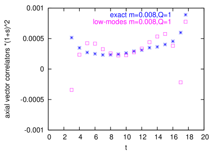
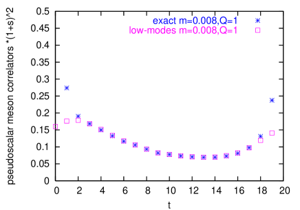
Figure 16: Triplet axial-vector (left) and pseudo-scalar (right) correlators at $am$ = 0.008 and $|Q|=1$. The low-mode-approximated correlator is compared with the corresponding exact one. The 20+$|Q|$ low-modes are not sufficient to evaluate the axial correlators but they are enough for the pseudo-scalar correlators at long distances.

A naive definition of the axial vector current is $A_{\mu}^{a}(x)=\bar{\psi}(x)\gamma_{5}\gamma_{\mu}(\tau^{a}/2)\psi(x)$, constructed from the overlap fermion field $\psi(x)$. Note that it is not the conserved current associated with the lattice chiral symmetry, and (finite) renormalization is needed to relate it to the continuum axial-vector current. We follow the method applied in Refs. [114, 115] to calculate the $Z_{A}$ factor non-perturbatively. Namely, we calculate

$$a\rho_{m}(t)\equiv\frac{a\sum_{\vec{x}}\langle\bar{\nabla}_{0}A^{a}_{0}(\vec{x},t)P^{a}(0,0)\rangle}{\sum_{\vec{x}}\langle P^{a}(\vec{x},t)P^{a}(0,0)\rangle},$$ (7.14)

where $\bar{\nabla}_{0}$ denotes a symmetric lattice derivative and $P^{a}(x)=\bar{\psi}(\tau^{a}/2)\gamma_{5}\psi$ .

Fitting the average of $\rho_{m}(t)$ over all topological sectors with a constant in the range $7\leq t\leq 13$, we obtain

$$a\rho(ma)\equiv\frac{a\langle\bar{\nabla_{\mu}}A^{a}_{\mu}(x)P^{a}(0)\rangle}{\langle P^{a}(x)P^{a}(0)\rangle}=\frac{2ma}{Z_{A}}+O(a^{2}),$$ (7.15)

at four quark masses $am$ = 0.0016, 0.0048, 0.008, 0.016, as plotted in Fig. 17, which shows a very good chiral behavior. With a quadratic fit we obtain

$$a\rho(ma)=0.00001(2)+1.390(14)(ma)-0.19(74)(ma)^{2}.$$ (7.16)

The constant term is perfectly consistent with zero and we extract an accurate value, $Z_{A}$ = 1.439(15) , which is consistent with the value $Z_{A}$ = 1.448(4) reported in Ref. [116] which was done with the same $\beta$ and $s$.

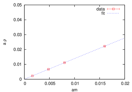
Figure 17: $a\rho$ as a function of the bare quark mass. Dashed line is a result of the quadratic fit: $a\rho=0.00001+1.390(ma)-0.19(ma)^{2}$.

Now one can compare the renormalized axial-vector correlation function with the qChPT result

$$2Z_{A}^{2}\sum_{\vec{x}}\langle A_{0}(\vec{x},t)A_{0}(0,0)\rangle^{Q}=2\left(\frac{F_{\pi}^{2}}{T}+2m\Sigma_{|Q|}(\mu)Th_{1}(|t/T|)\right).$$ (7.17)

to extract $F_{\pi}$ and $\Sigma$. In Ref. [55] it is reported that the correlators suffer from large statistical fluctuation when $|Q|=0$ and the data in the other topological sectors are insensitive to $\Sigma$, but it turned out that two-parameter ($F_{\pi}$ and $\Sigma$) fitting does work well when we treat the data of different topology and fermion masses simultaneously. As shown in Fig. 18, our data at $am$ = 0.0016, 0.0048, 0.008 in the $|Q|\leq 1$ sectors are well described by the qChPT formula (7.17). A simultaneous fit in the range $7\leq t\leq 13$ yields $F_{\pi}$ = 98.3(8.3) MeV and $\Sigma^{1/3}$ = 259(50) MeV with $\chi^{2}/\mbox{dof}$ = 0.19. The result for $F_{\pi}$ is in a good agreement with that of the previous work [57], 102(4) MeV.

On the other hand, the correlators at $|Q|$ = 2 do not agree with the above fit parameters as shown in Fig. 19. As discussed before, it may indicate that the topological sector $|Q|$ = 2 is already too large to apply the qChPT in the $\epsilon$-regime.

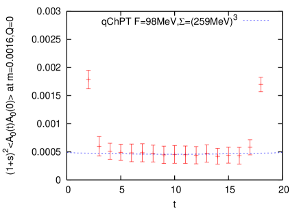
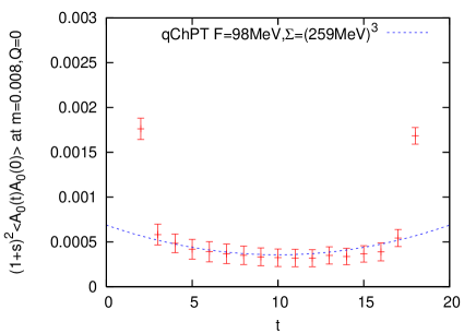
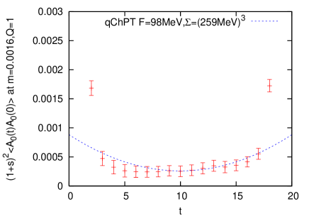
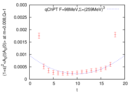
Figure 18: Axial-vector current correlators at $am$ = 0.0016 (left) and 0.008 (right) for $|Q|$ = 0 (top) and 1 (bottom). The dashed lines are the result of simultaneous fitting of the data for $Q$ = 0 and 1 at $am$ = 0.0016, 0.0048, 0.008 in the region $7\leq t\leq 13$.

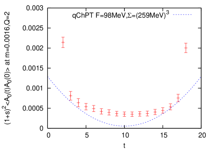
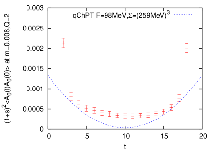
Figure 19: Axial-vector current correlators at $am$ = 0.0016 (left) and 0.008 (right) for $|Q|$ = 2. The dashed lines are the qChPT prediction with parameters determined through $|Q|$ = 0 and 1 sectors.

7.3.2 $\Sigma$, $\Sigma_{\mathrm{eff}}$ and $\alpha$ from connected S and PS correlators

We find that the scalar and pseudo-scalar triplet correlators are approximated precisely with the lowest 200$+|Q|$ eigen-modes at small quark masses ($m$ = 2.6–13 MeV) as the right panel of Fig.16 shows. In the range $7\leq t\leq 13$, the systematic error of this low-mode approximation is estimated to be only $1\%$ for the scalar correlators in $|Q|\geq 1$ sectors and the pseudo-scalar correlators in all the topological sectors. In this way we measure

$$\langle\mathcal{S}(t)\rangle^{Q}\equiv-2\sum_{\vec{x}}(1+s)^{2}\langle S^{3}(x+x_{0})S^{3}(x_{0})\rangle^{Q}_{\mathrm{low}},$$ (7.18)

$$\langle\mathcal{P}(t)\rangle^{Q}\equiv 2\sum_{\vec{x}}(1+s)^{2}\langle P^{3}(x+x_{0})P^{3}(x_{0})\rangle^{Q}_{\mathrm{low}},$$ (7.19)

at $am$ = 0.0016, 0.0032, 0.0048, 0.0064, and 0.008. We take an average of the source point $x_{0}$ over $(L/2)^{3}\times(T/2)$ lattice sites. In qChPT formulas (7.3) and (7.4), we have five parameters to be determined: $F_{\pi}$, $\Sigma$, $\Sigma_{\mathrm{eff}}$, $m_{0}^{2}$ and $\alpha$. Since these correlators are weakly depending on $F_{\pi}$, we use the jackknife samples of $F_{\pi}$ obtained from the axial-vector current correlator, $F_{\pi}$ = 98.3(8.3) MeV. Unfortunately, there still remain too many parameters to fit with qChPT expressions. Therefore, we use the relation (C.13) and an input $r_{0}^{4}\chi\equiv r_{0}^{4}\langle Q^{2}\rangle/V=0.059(3)$ from a recent work [117], which gives $m_{0}$ = 940(80)(23) MeV, where the second error reflects the error of $r_{0}^{4}\chi$.

With these input values, we fit the correlators (7.18) and (7.19) in the range $7\leq t\leq 13$ at different $Q$ and $m$ simultaneously. Fig. 20 shows the correlators with fitting curves. For $|Q|\leq 1$ sectors, the data at all available quark masses $am$ = 0.0016, 0.0032, 0.0064 and 0.008 are fitted well, and we actually get $\chi^{2}/\mathrm{dof}$ $\sim$ 0.7. (Note that the correlations between different $t$’s, $m$’s and channels (PS and S) are not taken into account.) This fit yields $\Sigma^{1/3}$ = 257 $\pm$ 14 $\pm$ 00 MeV, which is consistent with Ref. [96], $\Sigma_{\mathrm{eff}}^{1/3}$ = 271 $\pm$ 12 $\pm$ 00 MeV, and $\alpha$ = $-$4.5 $\pm$ 1.2 $\pm$ 0.2, where the first error is the statistical error and the second one is from uncertainty of $\langle Q^{2}\rangle$.

Here are some remarks. The ratio

$$\frac{\Sigma_{\mathrm{eff}}}{\Sigma}=1+\frac{1}{N_{c}F_{\pi}}\left(m_{0}^{2}\bar{G}(0)+\alpha\bar{\Delta}(0)\right),$$ (7.20)

should indicate the size of the NLO correction in the $\epsilon$ expansion. Our data, 1.163(59), implies that the $\epsilon$ expansion is actually converging. $\alpha$ has large negative value, which is also reported in Refs. [118] and [35]. These results contradict with a previous precise calculation [119], which obtained a smaller value $\alpha$ = 0.03(3). If we instead assume $\alpha$ = 0, and fit the data with $F_{\pi}$ as a free parameter, we obtain $F_{\pi}$ = 136.9(5.3) MeV and $\Sigma$ and $\Sigma_{\mathrm{eff}}$ are almost unchanged. (Detailed numbers are summarized in Table 11.) A possible cause is that $|Q|=1$ is not small enough to derive the partition function Eq.(C) (See Appendix C). Eq.(C.13) may also have a systematic error due to finite $V$ as well as finite $a$. Look at the data with $|Q|$ = 2, which are plotted in Fig. 20. They do not agree with expectations from the qChPT shown by dashed curves in the plots, which is also seen in the case with the axial-vector correlators. A simultaneous fit with all the data including $|Q|$ = 0, 1 and 2 gives a bad $\chi^{2}/\mathrm{dof}$ ($\simeq$ 12). Thus our numerical data might be posing a problem whether the partition function of qChPT $Z_{Q}$ is reliable or not, when $|Q|/\langle Q^{2}\rangle\ll 1$ is not satisfied very much; $\langle Q^{2}\rangle\sim 4.34(22)$ on our lattice.

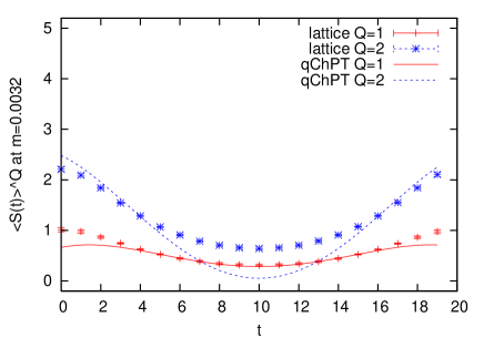
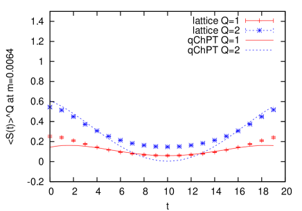
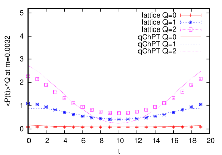
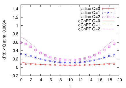
Figure 20: Scalar (top) and pseudo-scalar (bottom) correlators at $am$ = 0.0032 (left) and 0.0064 (right). The dotted lines are the fit results with all available mass parameters $am$ = 0.0016, 0.0032, 0.0064 and 0.008 for topological charges 0 and 1.

7.3.3 Chiral condensates

Consider the low-mode contribution to the scalar and pseudo-scalar condensates with a fixed topological charge $Q$,

$$\langle\bar{\psi}\psi(x)\rangle^{Q} = -\langle\mbox{tr}D_{m}^{-1}(x,x)\rangle^{Q}$$ (7.21)

$$= -\left\langle\mbox{tr}\left(\sum_{i=1}^{N_{\mathrm{low}}}\frac{1}{(1-\bar{a}m/2)\lambda_{i}+m}v_{i}(x)v_{i}^{\dagger}(x)+\Delta D_{m}^{-1}(x,x)\right)\right\rangle^{Q},$$

$$\langle\bar{\psi}\gamma_{5}\psi(x)\rangle^{Q} = -\langle\mbox{tr}\gamma_{5}D_{m}^{-1}(x,x)\rangle^{Q}$$

$$= -\left\langle\mbox{tr}\left(\sum_{i=1}^{N_{\mathrm{low}}}\frac{1}{(1-\bar{a}m/2)\lambda_{i}+m}\gamma_{5}v_{i}(x)v_{i}^{\dagger}(x)+\gamma_{5}\Delta D_{m}^{-1}(x,x)\right)\right\rangle^{Q}.$$

If $N_{\mathrm{low}}$ is large enough, the higher mode contribution, $\Delta D_{m}^{-1}(x,x)$, should be insensitive to the link variables $U_{\mu}(y)$ if $|y-x|\gg 0$ and thus to the global structure of the gauge field configuration, such as the topological charge. We, therefore, expect that the difference of the scalar condensates with different topology can be approximated with low-modes,

$$-(\langle\bar{\psi}\psi(x)\rangle^{Q}-\langle\bar{\psi}\psi(x)\rangle^{0})\sim-(\langle\bar{\psi}\psi(x)\rangle_{\mathrm{low}}^{Q}-\langle\bar{\psi}\psi(x)\rangle_{\mathrm{low}}^{0}).$$ (7.23)

In fact, Fig.21 shows that the convergence up to $N_{\mathrm{low}}=200+|Q|$ is really good. For the pseudo-scalar condensate, the situation is much easier, since the condensate is determined by the zero modes only;

$$-\langle\bar{\psi}\gamma_{5}\psi\rangle_{Q}=\frac{Q}{mV}.$$ (7.24)

Note that the contributions from non-zero eigen-modes cancel because of the orthogonality among different eigenvectors. As shown in Fig. 22, our data with $N_{\mathrm{low}}=200+|Q|$ low-modes perfectly agree with this theoretical expectation.

The free parameter in the scalar condensate is $\Sigma_{\mathrm{eff}}$ as seen in (7.1) and (C.16). We compare our numerical result of Eq.(7.23) with the qChPT result $\Sigma_{Q}(\mu^{\prime})-\Sigma_{Q=0}(\mu^{\prime})$. We use the low-mode averaging over $(L/2)^{3}\times(T/2)$ lattice sites. Fig. 23 shows the results as a function of quark mass for $|Q|$ = 1, 2 and 3. The lattice data agree remarkably well with the qChPT expectation with $\Sigma_{\mathrm{eff}}$ = 271(12) MeV as determined from the (pseudo-)scalar connected correlators as presented in the previous section. In fact, if we fit these data with $\Sigma_{\mathrm{eff}}$ as a free parameter, we obtain 256(14) MeV which is consistent with the result above.

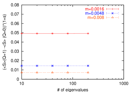
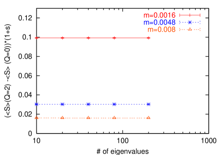
Figure 21: Low-mode dominance of $-(\langle\bar{\psi}\psi\rangle_{\mathrm{low}}^{Q}-\langle\bar{\psi}\psi\rangle_{\mathrm{low}}^{0})$ as a function of $N_{\mathrm{low}}$. The data are averaged over 20 configurations at $Q=1$ (left) and $Q=2$ (right).

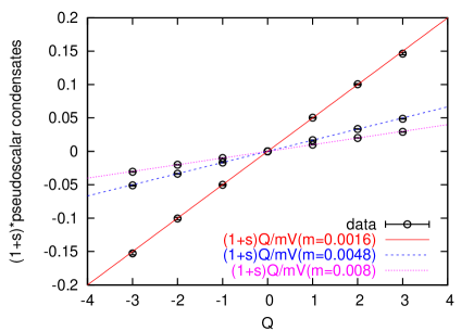
Figure 22: Pseudo-scalar condensates approximated with $N_{\mathrm{low}}=200+|Q|$ low-modes. The lines represent the expectation (7.24).

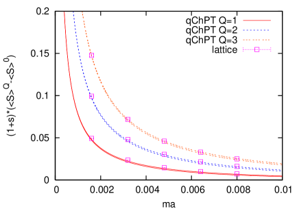
Figure 23: $-(\langle\bar{\psi}\psi\rangle^{Q}-\langle\bar{\psi}\psi\rangle^{0})$ as a function of quark mass. Data points are at $am$ = 0.0016, 0.0032, 0.0048, 0.0064, 0.008. The lines are qChPT predictions with $\Sigma_{\mathrm{eff}}^{1/3}$ = 271(12) MeV.

7.3.4 Disconnected PS correlators

Let us rewrite the disconnected pseudo-scalar correlator in a fixed topological sector,

$$\langle P(t)P(0)\rangle_{\mathrm{disc}}^{Q} \equiv \left\langle\sum_{\vec{x}}\mbox{tr}\left(\gamma_{5}D_{m}^{-1}(\vec{x},t;\vec{x},t)\right)\mbox{tr}\left(\gamma_{5}D_{m}^{-1}(\vec{0},0;\vec{0},0)\right)\right\rangle^{Q},$$ (7.25)

$$\stackrel{{\scriptstyle t\gg 0}}{{\longrightarrow}} \left\langle\sum_{\vec{x}}\mbox{tr}\left(\gamma_{5}\sum_{i=1}^{200+|Q|}\frac{1}{(1-\bar{a}m/2)\lambda_{i}+m}v_{i}(x)v_{i}^{\dagger}(x)\right)\right.$$

$$\left.\times\mbox{tr}\left(\gamma_{5}\sum_{i=1}^{200+|Q|}\frac{1}{(1-\bar{a}m/2)\lambda_{i}+m}v_{i}(0)v_{i}^{\dagger}(0)\right)\right\rangle^{Q}$$

$$+ 2\left\langle\mbox{tr}\left(\gamma_{5}\Delta D_{m}^{-1}(x,x)\right)\right\rangle^{\prime}$$

$$\times\left\langle\mbox{tr}\left(\gamma_{5}\sum_{i=1}^{200+|Q|}\frac{1}{(1-\bar{a}m/2)\lambda_{i}+m}v_{i}(0)v_{i}^{\dagger}(0)\right)\right\rangle^{Q}$$

$$+ \left[\left\langle\mbox{tr}\left(\gamma_{5}\Delta D_{m}^{-1}(x,x)\right)\right\rangle^{\prime}\right]^{2},$$

where $x=(\vec{x},t)$. Here we assume that higher mode’s contribution does not have correlation with any local operator $O(y)$ separated enough from $x$, i.e.

$$\langle\Delta D_{m}^{-1}(x,x)O(y)\rangle^{Q}\stackrel{{\scriptstyle|x-y|\gg 0}}{{\longrightarrow}}\langle\Delta D_{m}^{-1}(x,x)\rangle^{\prime}\times\langle O(y)\rangle^{Q},$$ (7.26)

where the expectation value $\langle\cdots\rangle^{\prime}$ represents insensitivity to the topological charge. We also use the translational invariance $\langle O(x)\rangle=\langle O(0)\rangle$. Since we know $\langle\mbox{tr}\left(\gamma_{5}\Delta D_{m}^{-1}(x,x)\right)\rangle^{\prime}=0$, the above equation should be well approximated with low-modes. In fact, Fig. 24 shows a very good convergence with the lowest 200+$|Q|$ eigen-modes. Similar results were also obtained previously in the study of the $\eta^{\prime}$ propagator with the Wilson fermion [111] and with the overlap fermion [120].

In the qChPT the correlator is written as

$$\langle\mathcal{P}^{d}(t)\rangle^{Q} \equiv \int\!d^{3}x\,(1+s)^{2}\langle 2P^{3}(x)P^{3}(0)-P^{0}(x)P^{0}(0)\rangle^{Q}$$ (7.27)

$$= \int\!d^{3}x\,(1+s)^{2}\left[C_{P}^{d}-\frac{\Sigma^{2}}{2F_{\pi}^{2}}\left(\frac{d_{+}}{N_{c}}(m_{0}^{2}\bar{G}(x)+\alpha\bar{\Delta}(x))-e_{+}\bar{\Delta}(x)\right)\right],$$

where

$$C_{P}^{d}=\frac{Q^{2}}{m^{2}V^{2}}, d_{+}=-4\left(1+\frac{Q^{2}}{\mu^{2}}\right), e_{+}=-2\left(\left(\frac{\Sigma_{Q}(\mu)}{\Sigma}\right)^{\prime}-\frac{\Sigma_{Q}(\mu)}{\mu\Sigma}\right).$$ (7.28)

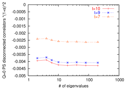
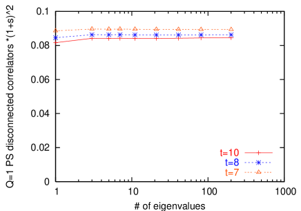
Figure 24: Convergence of the pseudo-scalar disconnected correlators for one sample configuration at $am=0.008$ for $Q=0$ (left) and $Q=1$ (right).

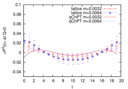
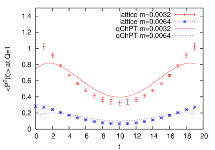
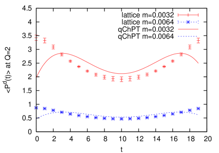
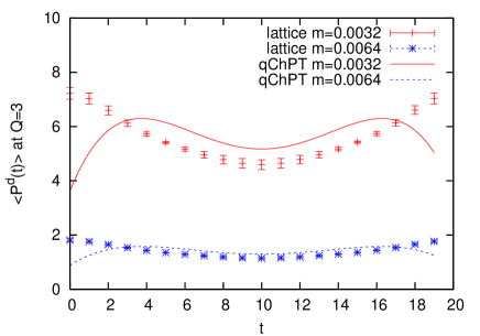
Figure 25: Disconnected pseudo-scalar correlators in the $0\leq|Q|\leq 3$ sectors at $am$ = 0.0032 and 0.0064. The curves represent the results of qChPT with $\Sigma^{1/3}$ = 257 MeV, $F_{\pi}$ = 98.3 MeV, $m_{0}$ = 940 MeV and $\alpha$ = $-$4.5.

In Fig. 25, we present the data in $|Q|$ = 0–3 topological sectors at two representative quark masses $am$ = 0.0032 and 0.0064. The qChPT predictions are plotted with the parameters determined from the axial-vector and (pseudo-)scalar connected correlators: $\Sigma^{1/3}$ = 257 MeV, $F_{\pi}$ = 98.3 MeV, $m_{0}$ = 940 MeV, and $\alpha$ = $-$4.5. One finds that the agreement is marginal, though the correlator’s magnitude and shape are qualitatively well described. Instead, if we fit the disconnected correlator with $\Sigma$ and $\alpha$ as free parameters while fixing $F_{\pi}$ and $m_{0}$ to the same value, we obtain $\Sigma^{1/3}$ = 227(32) MeV and $\alpha$ = $-$3.5(1.2), which are statistically consistent with those input numbers. We conclude that not only the connected correlators, but also disconnected correlators can be consistently expressed by the qChPT in the $\epsilon$-regime when $|Q|$ is small. Details of the fit results are listed in Table 11.

Table 11: Summary of the fitting results in the $\epsilon$-regime. The first column denotes the topological sectors used in the fit. The values in $[\cdots]$ are input parameters. The first error is statistical. The second and third errors reflect the uncertainty in the input parameters, $\langle Q^{2}\rangle$ and $F_{\pi}$, respectively.

correlators	$F_{\pi}$(MeV)	$\Sigma^{1/3}$ (MeV)	$\Sigma_{\mathrm{eff}}^{1/3}$ (MeV)	$\alpha$	$m_{0}$ (MeV)	$\chi^{2}/\mathrm{dof}$
axial vector
$|Q|=0$	98(17)	279(65)				0.02
$0\leq|Q|\leq 1$	98.3(8.3)	259(50)				0.19
$0\leq|Q|\leq 2$	117.9(4.3)	335(16)				2.8
connected PS+S
$0\leq|Q|\leq 1$	[98.3(8.3)]	257(14)(00)	271(12)(00)	$-$4.5(1.2)(0.2)	[940(80)(23)]	0.7
$0\leq|Q|\leq 1$	136.9(5.3)(0.9)	250(13)(00)	258(11)(00)	[0]	[674(26)(16)]	0.3
$0\leq|Q|\leq 2$	[98.3(8.3)]	258(12)(00)	264(11)(00)	$-$3.8(0.5)(0.2)	[940(80)(23)]	11.8
disconnected PS
$0\leq|Q|\leq 1$	[98.3(8.3)]	227(32)(00)		$-$3.5(1.2)(0.3)	[940(80)(23)]	1.0
$0\leq|Q|\leq 1$	125.7(5.6)(0.9)	223(29)(00)		[0]	[734(33)(14)]	0.7
$0\leq|Q|\leq 2$	[98.3(8.3)]	229(33)(00)(03)		$-$3.6(0.2)(0.3)(1.0)	[940(80)(23)]	1.0
$0\leq|Q|\leq 2$	135.0(4.9)(1.4)	237(32)(00)		[0]	[684(25)(13)]	1.7
$0\leq|Q|\leq 3$	[98.3(8.3)]	229(33)(01)(05)		$-$3.6(0.1)(0.2)(0.8)	[940(80)(23)]	1.0
$0\leq|Q|\leq 3$	139.3(4.1)(1.4)	244(32)(00)		[0]	[663(19)(12)]	1.9
scalar condensate ($\langle\bar{\psi}\psi\rangle^{0}-\langle\bar{\psi}\psi\rangle^{Q}$)
$1\leq|Q|\leq 3$			256(14)			1.2

8 Conclusions and discussions

The exact chiral symmetry is established on the lattice, with the overlap Dirac operator which satisfies the Ginsparg-Wilson relation. However, the overlap Dirac operator becomes ill-defined at certain points where the zero-mode of $H_{W}$ appears. Also, practically, these points make the numerical study very difficult. One has to carefully evaluate the discontinuity of the overlap fermion determinant (reflection/refraction) and the polynomial or rational expression of the overlap Dirac operator itself goes worse near this discontinuity. In fact, these dangerous points are topology boundaries; it is known that crossing $H_{W}=0$ changes the index of the overlap Dirac operator, or topological charge.

In the continuum limit, $H_{W}=0$ is automatically excluded but it would be better if we can construct the lattice gauge theory which does not allow $H_{W}=0$ from the beginning with a finite lattice spacing. There have been proposed two promising strategies. One is the gauge action which satisfies Lüscher’s “admissibility” condition and the other is an additional fermion determinant, $\det H_{W}^{2}$. Both of them are designed for the use of the hybrid Monte Carlo algorithm, in which global and small (smooth) updates are performed. Therefore, we regard them as “topology conserving actions”. In this thesis, we have investigated the possibility of lattice QCD in a fixed topological sector. We studied the properties of the topology conserving actions with no light quarks (namely, pure $SU(3)$ theory.). Although the admissibility condition with small $\epsilon$ ($<$ 1/20) can strictly prohibit the topology changes, our interest is the case with $\epsilon\sim O(1)$ for practical purposes. In the (quenched) Hybrid Monte Carlo updates, we found that the topology change is strongly suppressed for $1/\epsilon$ = 2/3 and 1, compared to the standard Wilson plaquette gauge action. The topological charge seems more stable for finer lattices, and it is possible to preserve the topological charge for O(100)-O(1,000) HMC trajectories at $a\simeq$ 0.08 fm and $L\simeq$ 1.3 fm, which might be applicable to the $\epsilon$-regime. The action Eq.(2.15) has, thus, been proved to be useful to accumulate gauge configurations in a fixed topological sector. While the gauge action Eq.(2.15) with $1/\epsilon=1$ and 2/3 allows the topology changes, at times, the topology conservation with the fermion determinant $\det H_{W}^{2}$ seems perfect. The numerical cost for this determinant is, of course, much more expensive than the quenched case, but it would be negligible compared to the cost of the dynamical overlap fermion. The full QCD overlap fermion simulation with the additional determinant $\det H_{W}^{2}$ may be very efficient, if we can omit the reflection/refraction procedures.

To test their practical feasibility, we measured the heavy quark potential with these actions. The lattice spacing is determined from the Sommer scale $r_{0}$. With these measurements we also investigated the scaling violation at short and intermediate distances. The probe in the short range is the violation of the rotational symmetry, and a ratio $r_{c}/r_{0}$ of two different scale can be used for the intermediate distance. For both of these we found that the size of the scaling violation is comparable to the case with the Wilson plaquette gauge action, which is consistent with the expectation that the term with $1/\epsilon$ introduces a difference at most $O(a^{4})$ or the additional large negative mass Wilson fermions are decoupled. These actions show no disadvantage as far as Wilson loops are concerned. We also found that the perturbative expansion of the coupling (after mean-field improvement) shows very good convergence even if $1/\epsilon$ term is introduced. The coupling constant in a certain scheme at a given scale is consistent among different values of $1/\epsilon$.

As another advantage of the (approximate) topology conservation, the low-lying eigenvalues of the Wilson-Dirac operator in the negative mass regime is suppressed. This reduces the cost of the numerical implementation of the overlap-Dirac operator. We observed that the topology conserving actions have a gain about a factor 2–3 at the same lattice spacing compared to the standard Wilson gauge action. Comparison with the other improved gauge actions, such as the Lüscher-Weisz, Iwasaki and DBW2 would be interesting.

In a fixed topological sector, one of the very interesting applications would be the QCD in the $\epsilon$-regime. In the chiral limit, the (q)ChPT analysis shows that the meson correlators are largely affected by the fermion zero-modes, and thus by the topology of the background gauge field. In order to study lattice QCD in such a regime, the chiral symmetric Dirac operator is essential, otherwise the large lattice artifacts would contaminate the fundamental points of the analysis, such as the definition of the topological charge, or what is the zero-mode, etc. To demonstrate how much effective the overlap Dirac operator is, we studied the quenched QCD with very small quark masses in the range $2.6$–13MeV. In this chiral regime, we observed that the chiral behavior is really nice, as seen in, for example, accurate determination of $Z_{A}$, or the pseudo-scalar condensates $\bar{\psi}\gamma_{5}\psi$. We also found the importance of the low lying modes and used them to extract the low-energy constants. (Note that the low lying modes are not affected by the $a\to 0$ limit, since it would add higher modes only, which are irrelevant to the low energy dynamics.) From triplet meson correlators with $Q=0$ and 1, we extracted $F_{\pi}$ = 98.3(8.3) MeV, $\Sigma^{1/3}$ = 257(14)(00) MeV ($\Sigma_{\mathrm{eff}}^{1/3}$ = 271(12)(00) MeV), $m_{0}$ = 940(80)(23) MeV, and $\alpha$ = $-$4.5(1.2)(0.2). In these numerical results the second error reflects the error of $\langle Q^{2}\rangle$. We also obtained consistent results from disconnected pseudo-scalar correlator and the chiral condensates. Although we observed minor inconsistencies and problems due to finite $Q$ correction, which is a special restriction of the quenched ChPT, these remarkable successes would encourage us to go further to $N_{f}\neq 0$ full QCD in the $\epsilon$-regime.

The exact chiral symmetry with the overlap Dirac operator is surely a most remarkable progress in the lattice gauge theory and it would be more and more important in both of the numerical works and theoretical works, in the future. In order to perform the path integrals, one should, however, note the fact that there is several points where $H_{W}$ has zero modes, which makes the overlap Dirac operator ill-defined, its locality is doubtful, and the numerical cost is suddenly enhanced. Our observation shows that the lattice QCD with fixed topology would be one of interesting and promising solutions to this. A number of applications such as $\theta$-vacuum, finite temperatures, and so on, might be possible as well.

For the future works, we would like to give a few remarks.

We have observed a large $\beta$-shift when the negative mass Wilson fermion Eq.(2.18) is added, which may also cause a unwanted large scaling violation. We thus propose another “topology stabilizer” which would have effects on $H_{W}\sim 0$ modes only;

$$\det\frac{a^{2}H_{W}^{2}}{a^{2}H_{W}^{2}+a^{2}m_{t}^{2}},$$ (8.1)

where the denominator is corresponding to the twisted mass ghost [121, 122, 123]

with a large negative mass $-(1+s)/a$ and a small twisted mass $m_{t}$. The effect from both determinant should be canceled unless $H_{W}$ has small eigenvalues. Note that $\det H_{W}^{2}/(H_{W}^{2}+a^{2}m_{t}^{2})\to 1$ with $m_{t}$ fixed.

As a final remark, let us consider the contribution from different topological sectors. In each topological sector, one measures the expectation value of operator $O$ with a fixed topological charge,

$$\langle O\rangle^{Q} \equiv \frac{\int dU^{Q}O\det(D+m)^{N_{f}}e^{-S_{G}}}{\int dU^{Q}\det(D+m)^{N_{f}}e^{-S_{G}}}\equiv\frac{\int dU^{Q}O\det(D+m)^{N_{f}}e^{-S_{G}}}{Z^{Q}},$$ (8.2)

where $dU^{Q}$ denotes the integral over the gauge fields with topological charge $Q$ and $\det(D+m)^{N_{f}}$ is the determinant of $N_{f}$ flavor overlap fermion with quark mass $m$. In order to calculate the total expectation value (in $\theta$-vacuum);

$$\langle O\rangle^{\theta} = \frac{\sum_{Q}e^{i\theta Q}\int dU^{Q}O\det(D+m)^{N_{f}}e^{-S_{G}}}{\sum_{Q}e^{i\theta Q}\int dU^{Q}\det(D+m)^{N_{f}}e^{-S_{G}}}=\frac{\sum_{Q}e^{i\theta Q}\langle O\rangle^{Q}Z_{Q}/Z_{0}}{\sum_{Q}e^{i\theta Q}Z_{Q}/Z_{0}},$$ (8.3)

the ratio $Z_{Q}/Z_{0}$ has to be evaluated. In fact, there are several proposals to calculate this ratio of the partition function, including the tempering method [124, 125, 126, 127, 128]. Here, we would like to propose an easier method. With an assumption that the ratio should be Gaussian;

$$Z_{Q}/Z_{0}\propto\exp\left(-\frac{Q^{2}}{2\langle Q^{2}\rangle^{\theta=0}}\right),$$ (8.4)

in a large volume $V$, one only has to calculate the topological susceptibility [129, 130],

$$\chi=\frac{\langle Q^{2}\rangle^{\theta=0}}{V},$$ (8.5)

to evaluate the ratio $Z_{Q}/Z_{0}$ with any value of $Q$. In principle, the topological susceptibility can be evaluated with the local topological charge density operator $q(x)=-\mbox{Tr}\gamma_{5}\bar{a}D(x,x)/2$ in a semi-local region (assuming the cluster decomposition principle);

$$\chi=\int d^{4}x\langle q(x)q(0)\rangle^{\theta=0}=\int_{V^{\prime}}d^{4}x\langle q(x)q(0)\rangle^{\theta=0},$$ (8.6)

where $\int_{V^{\prime}}d^{4}x$ is performed over the small volume $V^{\prime}$ around the origin, where $V^{\prime}\gg 1/\Lambda_{QCD}$. Thus, if the topological susceptibility in a fixed topological sector,

$$\chi^{Q}\equiv\int_{V^{\prime}}d^{4}x\langle q(x)q(0)\rangle^{Q},$$ (8.7)

shows sufficiently small $Q$ dependence and the finite volume effects due to $V$ and $V^{\prime}$ are both negligible, then $\chi^{Q}$ should be a good approximation of $\chi$ . What we would like to emphasize here is that summing up all the topology with the weight $Z_{Q}/Z_{0}$ (in a $\theta$-vacuum) is not so difficult and maybe not so important unless $\theta$ term is considered, since $Z_{Q}/Z_{0}\to_{V\to\infty}1$, although the numerical studies has to be done in the future works to verify this quite optimistic argument. It seems an appropriate way to preserve the topology along the simulations, since any lattice gauge action would eventually create large barriers between the topological sectors in the continuum limit.

Appendix A Notations

Lorentz indices $\mu,\nu$ run from 0 to 3. The lattice spacing and size are denoted by $a$ and $L$ respectively. The gauge field $U_{\mu}(x)\in SU(3)$ is located on the link from $x$ to $x+\hat{\mu}a$, where $\hat{\mu}$ is the unit vector in direction $\mu$. The plaquette is denoted by $P_{\mu\nu}(x)=U_{\mu}(x)U_{\nu}(x+a\hat{\mu})U^{\dagger}_{\mu}(x+a\hat{\nu})U^{\dagger}_{\nu}(x)$. The fermion field $\psi(x)$ is located on the site $x$. The forward and backward covariant difference of the fermion field $\psi(x)$ are defined by

$$\nabla_{\mu}\psi(x) = \frac{U_{\mu}(x)\psi(x+\hat{\mu}a)-\psi(x)}{a},$$

$$\nabla_{\mu}^{*}\psi(x) = \frac{\psi(x)-U_{\mu}^{\dagger}(x)\psi(x-\hat{\mu}a)}{a}.$$ (A.1)

Euclidean Dirac matrix $\gamma_{\mu}$ satisfies

$$\gamma_{\mu}^{\dagger}=\gamma_{\mu},\;\;\;\{\gamma_{\mu},\gamma_{\nu}\}=2\delta_{\mu,\nu},\;\;\;\gamma_{5}=\gamma_{0}\gamma_{1}\gamma_{2}\gamma_{3}.$$ (A.2)

The expectation values of an operator $O$ with a fixed topology is denoted by $\langle O\rangle^{Q}$.

Appendix B The hybrid Monte Carlo algorithm

We explain how to generate the configurations in our numerical simulations. The hybrid Monte Carlo algorithm (HMC) is one of the most efficient [25] algorithms and widely used in the lattice QCD studies.

Consider updating fields, $q_{i}$’s, which have an action $S(q)$. The HMC algorithm consists of two parts;

1. generate a candidate of updating field $q_{i}^{c}$.

2. judge whether $q_{i}^{c}$ is accepted or rejected.

The former is called molecular dynamics steps, since it is very similar to the trajectory of a classical particle, randomly walking in configuration space, of which path is determined by the equation of motion;

$$\frac{dq_{i}(\tau)}{d\tau}=\pi_{i}(\tau), \frac{d\pi_{i}(\tau)}{d\tau}=-\frac{\partial S(q)}{\partial q_{i}}(\tau),$$ (B.1)

where the initial momentum $\pi_{i}(\tau=0)$ is randomly given with probability density

$$P(\{\pi_{i}(0)\})=\left(\prod_{i}\frac{1}{\sqrt{2\pi}}\exp(-\sum_{i}\pi_{i}^{2}(0)/2)\right).$$ (B.2)

The final point, $q_{i}(\tau=\tau_{f})$, obtained in this way (after a fixed ’time’ $\tau_{f}$), is chosen to be the candidate $q_{i}^{c}$. This step is known to satisfy “the detailed balance” which is a sufficient condition for an algorithm to sample the distribution with the correct Boltzmann weight $\exp(-S(q))$. However, in the numerical studies, the evolution is done by the leap-frog updates with a finite step-size $\Delta\tau$,

$$q_{i}(\tau+\Delta\tau)-q_{i}(\tau) = \Delta\tau*\pi_{i}(\tau+\Delta\tau/2),$$

$$\pi_{i}(\tau+\Delta\tau/2)-\pi_{i}(\tau-\Delta\tau/2) = -\Delta\tau*\frac{\partial S(q)}{\partial q_{i}}(\tau).$$ (B.3)

Therefore, one needs the latter procedure, or the Metropolis test, to judge that the new configuration is accepted or not; $q_{i}^{c}$ is accepted with probability

$$P=\mbox{min}\left\{1,\frac{e^{-\pi_{i}^{c2}/2-S(q^{c})}}{e^{-\pi_{i}^{2}/2-S(q)}}\right\},$$ (B.4)

which realizes the exact detailed-balance. The above steps ($N_{mds}$ molecular dynamics steps with the step-size $\Delta\tau$ and the Metropolis test) are done in every ’trajectory’. In this way, the configurations are generated performing the hundreds or thousands of trajectories, $N_{\mathrm{trj}}$.

Let us consider the path integral

$$Z = \int dU_{\mu}\exp(-S_{G})\det(D+m)^{2}$$ (B.5)

$$= \int dU_{\mu}\exp(-S_{G})\int d\phi d\phi^{*}\exp\left(-\int d^{4}x\phi(x)^{*}((D+m)^{2})^{-1}\phi(x)\right),$$

where the pseudo-fermion field $\phi$ is introduced to evaluate the fermion determinant $\det(D+m)^{2}$, which can not be directly calculated when the lattice size is large.

Since the pseudo-fermion part of the action is a simple bilinear, $\phi$ can be updated with a conventional heat-bath algorithm. The HMC algorithm is applied to updating the link fields $U_{\mu}$’s with fixed $\phi=\phi_{h}$ which is generated by the heat-bath method;

$$Z_{\phi_{h}} = \int dU_{\mu}\exp(-S_{G})\exp\left(-\int d^{4}x\phi_{h}(x)^{*}(H_{W}^{2})^{-1}\phi_{h}(x)\right)$$ (B.6)

$$\equiv \int dU_{\mu}\exp(-S^{\phi_{h}}_{\mathrm{eff}}(U_{\mu})).$$

Thus, our lattice QCD simulation is performed as follows,

1. Choose a starting link variable configuration.

2. Choose $\eta\equiv(D+m)^{-1}\phi_{h}$ to be a field of Gaussian noise (heat-bath).

3. Choose the momentum of link variables, $\pi_{\mu}(x)$ from a Gaussian noise.

4. $N_{mds}$ molecular dynamics with the step-size $\Delta\tau$ are done.

5. Accept or reject the new configuration (Metropolis test).

6. Store the (new or old) configuration.

7. Return to step 2.

Note that both of

$$S^{\phi_{h}}_{eff},\;\;\;\mbox{and}\;\;\;\frac{\partial S^{\phi_{h}}_{eff}}{\partial U_{\mu}}$$ (B.7)

involves the calculation of $(D+m)^{-1}$, which requires a very expensive computational cost in the chiral limit, $m\to 0$, since a lot of low eigenvalues appear. Also, it is notable that when $(D+m)$ is not smooth with respect to the gauge link field $U_{\mu}$, sudden jumps of momentum evolution in Eq.(B.3) should be monitored, otherwise over(under) estimation of the momentum would break the algorithm. Finally, we should refer to the fact that each step of HMC is small variation of the fields, and therefore, tends to keep the initial topological properties of the link variables.

Appendix C Quenched chiral perturbation theory in the $\epsilon$-regime

This appendix is devoted to a brief review of quenched chiral perturbation theory (qChPT) in the $\epsilon$-regime [107] and we summarize the relevant formulas for our analysis of meson correlation functions.

The partition function of qChPT with $N_{v}$ valence quarks is defined

$$Z(\theta,M) = \int dU\exp\left(-\int d^{4}x\mathcal{L}^{\theta}_{M}(x)\right),$$ (C.1)

where the Lagrangian $\mathcal{L}^{\theta}_{M}$ is given by

$$\mathcal{L}^{\theta}_{M}(x) = \frac{F_{\pi}^{2}}{4}\mbox{Str}(\partial_{\mu}U(x)^{-1}\partial_{\mu}U(x))-\frac{m\Sigma}{2}\mbox{Str}(U_{\theta}U(x)+U(x)^{-1}U_{\theta}^{-1})$$ (C.2)

$$+\frac{m_{0}^{2}}{2N_{c}}\Phi(x)^{2}+\frac{\alpha}{2N_{c}}\partial_{\mu}\Phi(x)\partial_{\mu}\Phi(x),$$

at the leading order of pion mass, $m_{\pi}^{2}$, and pion momentum, $p_{\pi}^{2}$, expansion, where $N_{c}$ denotes the number of color, $F_{\pi}$ is the pion decay constant and $\Sigma$ is the chiral condensate. $U(x)$ is integrated over a sub-manifold of the super-group $Gl(N_{v}|N_{v})$, called the maximally symmetric Riemannian sub-manifold which is characterized by a matrix of form

$$U=\left(\begin{array}[]{cc}A&B\\ C&D\end{array}\right),\;\;\;\;\;A\in U(N_{v}),\;\;\;\;\;D\in Gl(N_{v})/U(N_{v}),$$ (C.3)

and Grassmannian $N_{v}\times N_{v}$ matrices $B$ and $C$. Str denotes the super-trace. The quark mass is involved in the mass matrix $M=(mI_{v}+m\tilde{I_{v}})$ where $I_{v}$ and $\tilde{I_{v}}$ are the identity matrix in the fermion-fermion and boson-boson blocks respectively. The $\theta$ term which violates CP symmetry, enters through $U_{\theta}\equiv\exp(i\theta/N_{v})I_{N_{v}}+\tilde{I}_{N_{v}}$. Note that in the quenched approximation the singlet field $\Phi(x)\equiv\frac{F_{\pi}}{\sqrt{2}}\mbox{Str}[-i\ln U(x)]$ is not decoupled, and its mass $m_{0}^{2}$ and coupling $\alpha$ are introduced [132].

The $\epsilon$-regime [43, 44, 45, 46, 47, 48] is a special regime where the quark mass is so small that the pion Compton wavelength $\sim 1/m_{\pi}$ is larger than the linear extent of the space-time $L$. In this regime, the zero mode of pion gives important contribution and one must explicitly integrate out the constant mode of $U(x)$. The other mode’s contributions are perturbatively evaluated with the expansion parameter, $\epsilon^{2}\sim m_{\pi}/4\pi F_{\pi}\sim 1/(LF_{\pi})^{2}$. Namely, separating the zero mode and the other modes;

$$U(x)=U_{0}\exp i\frac{\sqrt{2}\xi(x)}{F_{\pi}},$$ (C.4)

the Lagrangian Eq.(C.2) can be rewritten. Together with $\epsilon$-expansion, one obtains the partition function with a fixed topological charge $Q$ by Fourier transforming (C.1) as follows,

$$Z_{Q}(M) \equiv \frac{1}{2\pi}\int^{\pi}_{-\pi}\!d\theta e^{i\theta Q}Z(\theta,M)$$ (C.5)

$$= \frac{1}{2\pi}\int^{\pi}_{-\pi}\!d\theta\int dU^{\prime}_{0}d\xi(\mbox{Sdet}U_{0}^{\prime})^{Q}\exp\left[-\int d^{4}x\left(\mathcal{L}^{\theta}_{M}(x)+i\frac{\sqrt{2}Q}{F_{\pi}V}\Phi_{0}\right)\right]$$

$$= \frac{1}{2\pi}\int^{\pi}_{-\pi}\!d\theta\int dU^{\prime}_{0}d\xi(\mbox{Sdet}U_{0}^{\prime})^{Q}\exp\left[-\frac{Vm_{0}^{2}}{2N_{c}}\left(\Phi_{0}^{\prime}-\frac{F_{\pi}\theta}{\sqrt{2}}\right)^{2}-\frac{\sqrt{2}iQ}{F_{\pi}}\left(\Phi_{0}^{\prime}-\frac{F_{\pi}\theta}{\sqrt{2}}\right)\right]$$

$$\times\exp\left[\frac{m\Sigma V}{2}\mbox{Str}(U_{0}^{\prime}+U_{0}^{\prime-1})\right.$$

$$\left.\;\;+\int d^{4}x\left(-\frac{1}{2}\mbox{Str}(\partial_{\mu}\xi\partial_{\mu}\xi)-\frac{m_{0}^{2}}{2N_{c}}(\mbox{Str}\xi)^{2}-\frac{\alpha}{2N_{c}}(\partial_{\mu}\mbox{Str}\xi)^{2}\right)\right]$$

$$= \frac{1}{\sqrt{2\pi\langle Q^{2}\rangle}}e^{-Q^{2}/2\langle Q^{2}\rangle}\int dU^{\prime}_{0}d\xi(\mbox{Sdet}U^{\prime}_{0})^{Q}\exp\left[\frac{m\Sigma V}{2}\mbox{Str}(U^{\prime}_{0}+U^{\prime-1}_{0})\right.$$

$$+\left.\int d^{4}x\left(-\frac{1}{2}\mbox{Str}(\partial_{\mu}\xi\partial_{\mu}\xi)-\frac{m_{0}^{2}}{2N_{c}}(\mbox{Str}\xi)^{2}-\frac{\alpha}{2N_{c}}(\partial_{\mu}\mbox{Str}\xi)^{2}\right)+O(\epsilon^{4})\right],$$

where we use

$$U = U_{0}e^{i\sqrt{2}\xi/F_{\pi}},$$ (C.6)

$$\Phi_{0} \equiv \frac{F_{\pi}}{\sqrt{2}}\mbox{Str}(-i\ln U_{0}),$$ (C.7)

$$U_{0}^{\prime} = U_{\theta}U_{0},$$ (C.8)

$$e^{iQ\theta} = (\mbox{Sdet}U_{0}^{\prime})^{Q}\exp\left(-\int d^{4}x\frac{\sqrt{2}iQ}{F_{\pi}V}\Phi_{0}\right),$$ (C.9)

$$\Phi_{0}^{\prime} \equiv \frac{F_{\pi}}{\sqrt{2}}\mbox{Str}(-i\ln U_{0}^{\prime})=\Phi_{0}+\frac{F_{\pi}\theta}{\sqrt{2}}.$$ (C.10)

In the last line of (C.5), we perform $\theta$ integral as a Gaussian;

$$\frac{1}{2\pi}\int^{\pi}_{-\pi}d\theta\exp\left[-\frac{Vm_{0}^{2}F_{\pi}^{2}}{4N_{c}}\left(\theta-\frac{\sqrt{2}}{F_{\pi}}\Phi_{0}^{\prime}\right)^{2}+iQ\left(\theta-\frac{\sqrt{2}}{F_{\pi}}\Phi_{0}^{\prime}\right)\right]$$ (C.11)

$$= \exp\left(-\frac{Q^{2}}{2\langle Q^{2}\rangle}\right)\frac{1}{2\pi}\int^{\pi}_{-\pi}d\theta^{\prime}\exp\left[-\frac{\langle Q^{2}\rangle}{2}\left(\theta^{\prime}-\frac{iQ}{\langle Q^{2}\rangle}\right)^{2}\right]$$

$$\sim \frac{1}{\sqrt{2\pi\langle Q^{2}\rangle}}\exp\left(-\frac{Q^{2}}{2\langle Q^{2}\rangle}\right),$$

where $\langle Q^{2}\rangle=Vm_{0}^{2}F_{\pi}^{2}/2N_{c}$ and $\theta^{\prime}=\theta-\sqrt{2}\Phi^{\prime}_{0}/F_{\pi}$. We need a condition, $|Q|/\langle Q^{2}\rangle\ll 1$, in order to justify this Gaussian integral, otherwise the integral Eq.(C.11) should depend on $\Phi_{0}^{\prime}$, which means that $\Phi_{0}^{\prime}$ and $\theta$ can not be treated independently and the last line of the partition function Eq.(C.5) is invalid. Therefore, all the results shown below are reliable only for small $|Q|$.

With redefinition $U_{0}^{\prime}=U_{0}$, the partition function in a fixed topological sector is obtained

$$Z_{Q}(M) \equiv \frac{1}{2\pi}\int_{-\pi}^{+\pi}\!d\theta e^{i\theta Q}Z(\theta,M)$$

$$= \frac{1}{\sqrt{2\pi\langle Q^{2}\rangle}}e^{-Q^{2}/2\langle Q^{2}\rangle}\int dU_{0}d\xi\,(\mathrm{S}\det U_{0})^{Q}\exp\left[\frac{m\Sigma V}{2}\mbox{Str}(U_{0}+U_{0}^{-1})\right.$$

$$+\left.\int\!d^{4}x\left(-\frac{1}{2}\mbox{Str}(\partial_{\mu}\xi\partial_{\mu}\xi)-\frac{m_{0}^{2}}{2N_{c}}(\mbox{Str}\xi)^{2}-\frac{\alpha}{2N_{c}}(\partial_{\mu}\mbox{Str}\xi)^{2}\right)+O(\epsilon^{4})\right],$$

where $dU_{0}$ denotes the Haar measure of the maximally Riemannian sub-manifold of
$Gl(N_{v}|N_{v})$. Note that the topological charge distributes as a Gaussian with variance

$$\frac{\langle Q^{2}\rangle}{V}=\frac{F_{\pi}^{2}m_{0}^{2}}{2N_{c}},$$ (C.13)

which is in a good contrast with the full theory, for which $\langle Q^{2}\rangle=m\Sigma V/N_{f}$ is expected with $N_{f}$ flavors.

In the following we consider $N_{v}$ = 1 and 2 cases only, as we are interested in the system with two light quarks. Any correlators or condensates are obtained by the perturbation of $\xi$ fields and the exact integration over zero mode, $U_{0}$, which can be written in terms of the Bessel functions.

First let us calculate the condensates. At the tree-level the scalar condensate is given by

$$-\langle\bar{\psi}\psi\rangle_{Q}\equiv\Sigma_{Q}(\mu)=\Sigma\mu(I_{|Q|}(\mu)K_{|Q|}(\mu)+I_{|Q|+1}(\mu)K_{|Q|-1}(\mu))+\Sigma\frac{|Q|}{\mu},$$ (C.14)

with $\mu\equiv m\Sigma V$. $I_{|Q|}(\mu)$ and $K_{|Q|}(\mu)$ denote the modified Bessel functions. One-loop contribution does not change its functional form [133]

$$\Sigma^{\mathrm{1-loop}}_{Q}(\mu)=\Sigma_{\mathrm{eff}}\mu^{\prime}(I_{|Q|}(\mu^{\prime})K_{|Q|}(\mu^{\prime})+I_{|Q|+1}(\mu^{\prime})K_{|Q|-1}(\mu^{\prime}))+\Sigma_{\mathrm{eff}}\frac{|Q|}{\mu^{\prime}}=\Sigma_{Q}(\mu^{\prime}),$$ (C.15)

but the parameters $\mu$ and $\Sigma$ are shifted to $\mu^{\prime}$ and $\Sigma_{\mathrm{eff}}$:

$$\mu^{\prime}\equiv m\Sigma_{\mathrm{eff}}V, \Sigma_{\mathrm{eff}}\equiv\Sigma\left(1+\frac{m_{0}^{2}\bar{G}(0)+\alpha\bar{\Delta}(0)}{N_{c}F_{\pi}^{2}}\right).$$ (C.16)

Here, parameters $\bar{G}(0)$ and $\bar{\Delta}(0)$ are ultraviolet divergent tadpole integrals,

$$\bar{G}(x)\equiv\frac{1}{V}\sum_{p\neq 0}\frac{e^{ipx}}{p^{4}}, \bar{\Delta}(x)\equiv\frac{1}{V}\sum_{p\neq 0}\frac{e^{ipx}}{p^{2}},$$ (C.17)

which need renormalization.

Next, we consider the flavor-singlet meson operators

$$S^{0}(x)\equiv\bar{\psi}(x)I_{N_{V}}\psi(x), P^{0}(x)\equiv\bar{\psi}(x)i\gamma_{5}I_{N_{V}}\psi(x).$$ (C.18)

To add these operators to the QCD Lagrangian as source terms;

$$\mathcal{L}\to\mathcal{L}+s(x)S^{0}(x)+p(x)P^{0}(x),$$ (C.19)

corresponds to the substitution

$$M\to M+s(x)I_{N_{v}}+ip(x)I_{N_{v}}$$ (C.20)

in qChPT. The two-point correlation functions are obtained by differentiating the generating functional by $s(x)$ and $p(x)$. To $O(\epsilon^{2})$ the results are

$$\langle S^{0}(x)S^{0}(0)\rangle_{Q} = C_{S}^{0}+\frac{\Sigma^{2}}{2F_{\pi}^{2}}\left[\frac{a_{-}}{N_{c}}(m_{0}^{2}\bar{G}(x)+\alpha\bar{\Delta}(x))-\bar{\Delta}(x)\frac{a_{+}+a_{-}-4}{2}\right],$$ (C.21)

$$\langle P^{0}(x)P^{0}(0)\rangle_{Q} = C_{P}^{0}-\frac{\Sigma^{2}}{2F_{\pi}^{2}}\left[\frac{a_{+}}{N_{c}}(m_{0}^{2}\bar{G}(x)+\alpha\bar{\Delta}(x))-\bar{\Delta}(x)\frac{a_{+}+a_{-}+4}{2}\right],$$ (C.22)

where

$$a_{+}=4\left[\left(\frac{\Sigma_{Q}(\mu)}{\Sigma}\right)^{\prime}+1+\frac{Q^{2}}{\mu^{2}}\right], a_{-}=4\left[-\frac{1}{\mu}\frac{\Sigma_{Q}(\mu)}{\Sigma}+1+\frac{Q^{2}}{\mu^{2}}\right],$$ (C.23)

and the constant terms are given by

$$C_{S}^{0} = \frac{\Sigma^{2}_{\mathrm{eff}}}{4}a_{+}^{\mathrm{1-loop}}=\Sigma^{2}_{\mathrm{eff}}\left[\left(\frac{\Sigma_{Q}(\mu^{\prime})}{\Sigma_{\mathrm{eff}}}\right)^{\prime}+1+\frac{Q^{2}}{\mu^{\prime 2}}\right],$$ (C.24)

$$C_{P}^{0} = -\frac{\Sigma^{2}_{\mathrm{eff}}}{4}a_{-}^{\mathrm{1-loop}}=\Sigma^{2}_{\mathrm{eff}}\left[\frac{1}{\mu^{\prime}}\frac{\Sigma_{Q}(\mu^{\prime})}{\Sigma_{\mathrm{eff}}}-\frac{Q^{2}}{\mu^{\prime 2}}\right].$$ (C.25)

Note that the prime denotes the derivative with respect to $\mu$,

$$\left(\frac{\Sigma_{Q}(\mu)}{\Sigma}\right)^{\prime}=I_{|Q|}(\mu)K_{|Q|}(\mu)-I_{|Q|+1}(\mu)K_{|Q|-1}(\mu)-\frac{|Q|}{\mu^{2}}.$$ (C.26)

For flavor non-singlet case, we need a $N_{v}=2$ super-group integral, which is also described with the Bessel functions. The non-singlet operators are given by

$$S^{a}(x) \equiv \bar{\psi}(x)(\tau^{a}/2)I_{N_{V}}\psi(x),$$ (C.27)

$$P^{a}(x) \equiv \bar{\psi}(x)(\tau^{a}/2)i\gamma_{5}I_{N_{V}}\psi(x),$$ (C.28)

with the Pauli matrices $\tau^{a}$. To $O(\epsilon^{2})$ the two-point functions are given by

$$\langle S^{a}(x)S^{a}(0)\rangle_{Q} = C_{S}^{a}+\frac{\Sigma^{2}}{2F_{\pi}^{2}}\left[\frac{c_{-}}{N_{c}}(m_{0}^{2}\bar{G}(x)+\alpha\bar{\Delta}(x))-\bar{\Delta}(x)b_{-}\right],$$ (C.29)

$$\langle P^{a}(x)P^{a}(0)\rangle_{Q} = C_{P}^{a}-\frac{\Sigma^{2}}{2F_{\pi}^{2}}\left[\frac{c_{+}}{N_{c}}(m_{0}^{2}\bar{G}(x)+\alpha\bar{\Delta}(x))-\bar{\Delta}(x)b+\right],$$ (C.30)

where

$$b_{+}=2\left(1+\frac{Q^{2}}{\mu^{2}}\right),\;\;\;b_{-}=2\frac{Q^{2}}{\mu^{2}},\;\;\;c_{+}=2\left(\frac{\Sigma_{Q}(\mu)}{\Sigma}\right)^{\prime},\;\;\;c_{-}=-2\frac{1}{\mu}\frac{\Sigma_{Q}(\mu)}{\Sigma},$$ (C.31)

and

$$C_{S}^{a}=\frac{\Sigma^{2}_{\mathrm{eff}}}{2}\left(\frac{\Sigma_{Q}(\mu^{\prime})}{\Sigma_{\mathrm{eff}}}\right)^{\prime}, C_{P}^{a}=\frac{\Sigma^{2}_{\mathrm{eff}}}{2}\left(\frac{\Sigma_{Q}(\mu^{\prime})}{\mu^{\prime}\Sigma_{\mathrm{eff}}}\right).$$ (C.32)

For the flavor non-singlet axial-vector current

$$A_{\mu}^{a}(x)=\bar{\psi}(x)(\tau^{a}/2)i\gamma_{\mu}\gamma_{5}\psi(x),$$ (C.33)

the correlator is obtained [108]

$$\langle A^{a}_{0}(x)A^{a}_{0}(0)\rangle_{Q} = -\frac{F_{\pi}}{V}-2m\Sigma_{Q}(\mu)\bar{\Delta}(x).$$ (C.34)

An important observation here is that the axial-current correlator does not depend on the parameters related to the quenched artifact, i.e. $m_{0}^{2}$ and $\alpha$. Also note that the constant term is proportional to $F_{\pi}$ rather than $\Sigma$. Therefore, this channel is suitable for an extraction of $F_{\pi}$, whereas for the pseudo-scalar and scalar correlators $F_{\pi}$ appears only in the coefficients of $\bar{\Delta}(x)$ and $\bar{G}(x)$ terms.

For zero spatial momentum projection, it is convenient to define

$$h_{1}(|t/T|) = \frac{1}{T}\int\!d^{3}x\,\bar{\Delta}(x)=\frac{1}{2}\left[\left(\frac{|t|}{T}-\frac{1}{2}\right)^{2}-\frac{1}{12}\right],$$ (C.35)

$$h_{2}(|t/T|) = -\frac{1}{T^{3}}\int\!d^{3}x\,\bar{G}(x)=\frac{1}{24}\left[\frac{t^{2}}{T^{2}}\left(\frac{|t|}{T}-1\right)^{2}-\frac{1}{30}\right].$$ (C.36)

As a Remarkable feature in the $\epsilon$-regime, the correlators do not behave as the usual exponential fall-off $\exp(-Mt)$ with the mass gap $M$.

References

- [1] H. B. Nielsen and M. Ninomiya, Nucl. Phys. B 185, 20 (1981) [Erratum-ibid. B 195, 541 (1982)].
- [2] H. B. Nielsen and M. Ninomiya, Nucl. Phys. B 193, 173 (1981).
- [3] K. G. Wilson, CLNS-321 New Phenomena In Subnuclear Physics. Part A. Proceedings of the First Half of the 1975 International School of Subnuclear Physics, Erice, Sicily, July 11 - August 1, 1975, ed. A. Zichichi, Plenum Press, New York, 1977, p. 69, CLNS-321
- [4] H. Neuberger, Phys. Lett. B 417, 141 (1998) [arXiv:hep-lat/9707022].
- [5] H. Neuberger, Phys. Lett. B 427, 353 (1998) [arXiv:hep-lat/9801031].
- [6] D. B. Kaplan, Phys. Lett. B 288, 342 (1992) [arXiv:hep-lat/9206013].
- [7] Y. Shamir, Nucl. Phys. B 406, 90 (1993) [arXiv:hep-lat/9303005].
- [8] V. Furman and Y. Shamir, Nucl. Phys. B 439, 54 (1995) [arXiv:hep-lat/9405004].
- [9] U. J. Wiese, Phys. Lett. B 315, 417 (1993) [arXiv:hep-lat/9306003].
- [10] P. Hasenfratz, V. Laliena and F. Niedermayer, Phys. Lett. B 427, 125 (1998) [arXiv:hep-lat/9801021].
- [11] P. H. Ginsparg and K. G. Wilson, Phys. Rev. D 25, 2649 (1982).
- [12] M. Luscher, Phys. Lett. B 428, 342 (1998) [arXiv:hep-lat/9802011].
- [13] R. Narayanan, H. Neuberger and P. M. Vranas, Phys. Lett. B 353, 507 (1995) [arXiv:hep-lat/9503013].
- [14] H. Neuberger, Phys. Rev. D 60, 065006 (1999) [arXiv:hep-lat/9901003].
- [15] A. Bode, U. M. Heller, R. G. Edwards and R. Narayanan, arXiv:hep-lat/9912043.
- [16] Z. Fodor, S. D. Katz and K. K. Szabo, JHEP 0408, 003 (2004) [arXiv:hep-lat/0311010].
- [17] G. Arnold, N. Cundy, J. van den Eshof, A. Frommer, S. Krieg, T. Lippert and K. Schafer, arXiv:hep-lat/0311025.
- [18] N. Cundy, J. van den Eshof, A. Frommer, S. Krieg, T. Lippert and K. Schafer, Comput. Phys. Commun. 165, 221 (2005) [arXiv:hep-lat/0405003].
- [19] N. Cundy, S. Krieg, G. Arnold, A. Frommer, T. Lippert and K. Schilling, arXiv:hep-lat/0502007.
- [20] T. DeGrand and S. Schaefer, Phys. Rev. D 71, 034507 (2005) [arXiv:hep-lat/0412005].
- [21] T. DeGrand and S. Schaefer, Phys. Rev. D 72, 054503 (2005) [arXiv:hep-lat/0506021].
- [22] S. Schaefer and T. DeGrand, PoS LAT2005, 140 (2005) [arXiv:hep-lat/0508025].
- [23] G. I. Egri, Z. Fodor, S. D. Katz and K. K. Szabo, JHEP 0601, 049 (2006) [arXiv:hep-lat/0510117].
- [24] N. Cundy, Nucl. Phys. Proc. Suppl. 153, 54 (2006) [arXiv:hep-lat/0511047].
- [25] S. Duane, A. D. Kennedy, B. J. Pendleton and D. Roweth, Phys. Lett. B 195, 216 (1987).
- [26] M. Luscher, Nucl. Phys. B 538, 515 (1999) [arXiv:hep-lat/9808021].
- [27] M. Luscher, Nucl. Phys. B 549, 295 (1999) [arXiv:hep-lat/9811032].
- [28] M. Luscher, Nucl. Phys. B 568, 162 (2000) [arXiv:hep-lat/9904009].
- [29] P. Hernandez, K. Jansen and M. Luscher, Nucl. Phys. B 552, 363 (1999) [arXiv:hep-lat/9808010].
- [30] H. Neuberger, Phys. Rev. D 61, 085015 (2000) [arXiv:hep-lat/9911004].
- [31] H. Fukaya and T. Onogi, Phys. Rev. D 68, 074503 (2003) [arXiv:hep-lat/0305004].
- [32] H. Fukaya and T. Onogi, D 70, 054508 (2004) [arXiv:hep-lat/0403024].
- [33] S. Shcheredin, W. Bietenholz, K. Jansen, K. I. Nagai, S. Necco and L. Scorzato, Nucl. Phys. Proc. Suppl. 140, 779 (2005) [arXiv:hep-lat/0409073].
- [34] W. Bietenholz, K. Jansen, K. I. Nagai, S. Necco, L. Scorzato and S. Shcheredin [XLF Collaboration], AIP Conf. Proc. 756, 248 (2005) [arXiv:hep-lat/0412017].
- [35] S. Shcheredin, arXiv:hep-lat/0502001.
- [36] K. i. Nagai, K. Jansen, W. Bietenholz, L. Scorzato, S. Necco and S. Shcheredin, Proc. Sci. LAT2005, 283 (2005) [arXiv:hep-lat/0509170].
- [37] H. Fukaya, S. Hashimoto, T. Hirohashi, K. Ogawa and T. Onogi, Phys. Rev. D 73, 014503 (2006) [arXiv:hep-lat/0510116].
- [38] W. Bietenholz, K. Jansen, K. I. Nagai, S. Necco, L. Scorzato and S. Shcheredin, arXiv:hep-lat/0511016.
- [39] M. Luscher, private communications.
- [40] P. M. Vranas, arXiv:hep-lat/0001006.
- [41] P. Hernandez, K. Jansen and M. Luscher, arXiv:hep-lat/0007015.
- [42] T. Izubuchi and C. Dawson [RBC Collaboration], Nucl. Phys. Proc. Suppl. 106, 748 (2002).
- [43] J. Gasser and H. Leutwyler, “Chiral Perturbation Theory To One Loop,” Annals Phys. 158, 142 (1984).
- [44] J. Gasser and H. Leutwyler, Phys. Lett. B 188, 477 (1987).
- [45] J. Gasser and H. Leutwyler, Nucl. Phys. B 307, 763 (1988).
- [46] F. C. Hansen, Nucl. Phys. B 345, 685 (1990).
- [47] F. C. Hansen and H. Leutwyler, Nucl. Phys. B 350, 201 (1991).
- [48] H. Leutwyler and A. Smilga, “Spectrum of Dirac operator and role of winding number in QCD,” Phys. Rev. D 46, 5607 (1992).
- [49] C. Gattringer, P. Huber and C. B. Lang [Bern-Graz-Regensburg (BGR) Collaboration], Phys. Rev. D 72, 094510 (2005) [arXiv:hep-lat/0509003].
- [50] C. Gattringer, P. Huber and C. B. Lang, PoS LAT2005, 121 (2005) [arXiv:hep-lat/0509059].
- [51] P. Hernandez, K. Jansen and L. Lellouch, “Finite-size scaling of the quark condensate in quenched lattice QCD,” Phys. Lett. B 469, 198 (1999) [arXiv:hep-lat/9907022].
- [52] S. Prelovsek and K. Orginos [RBC Collaboration], Nucl. Phys. Proc. Suppl. 119, 822 (2003) [arXiv:hep-lat/0209132].
- [53] L. Giusti, C. Hoelbling, M. Luscher and H. Wittig, Comput. Phys. Commun. 153, 31 (2003) [arXiv:hep-lat/0212012].
- [54] L. Giusti, M. Luscher, P. Weisz and H. Wittig, JHEP 0311, 023 (2003) [arXiv:hep-lat/0309189].
- [55] W. Bietenholz, T. Chiarappa, K. Jansen, K. I. Nagai and S. Shcheredin, JHEP 0402, 023 (2004) [arXiv:hep-lat/0311012].
- [56] L. Giusti, P. Hernandez, M. Laine, P. Weisz and H. Wittig, JHEP 0401, 003 (2004) [arXiv:hep-lat/0312012].
- [57] L. Giusti, P. Hernandez, M. Laine, P. Weisz and H. Wittig, JHEP 0404, 013 (2004) [arXiv:hep-lat/0402002].
- [58] K. Ogawa and S. Hashimoto, Prog. Theor. Phys. 114, 609 (2005) [arXiv:hep-lat/0505017].
- [59] H. Fukaya, S. Hashimoto and K. Ogawa, Prog. Theor. Phys. 114 (2005) 451 [arXiv:hep-lat/0504018].
- [60] T. Mehen and B. C. Tiburzi, Phys. Rev. D 72, 014501 (2005) [arXiv:hep-lat/0505014].
- [61] W. Bietenholz and S. Shcheredin, PoS LAT2005, 138 (2005) [arXiv:hep-lat/0508016].
- [62] L. Giusti and S. Necco, PoS LAT2005, 132 (2005) [arXiv:hep-lat/0510011].
- [63] P. H. Damgaard, U. M. Heller, K. Splittorff and B. Svetitsky, Phys. Rev. D 72, 091501 (2005) [arXiv:hep-lat/0508029].
- [64] W. Bietenholz and S. Shcheredin, Nucl. Phys. Proc. Suppl. 153, 17 (2006) [arXiv:hep-lat/0511051].
- [65] S. Shcheredin and W. Bietenholz, PoS LAT2005, 134 (2005) [arXiv:hep-lat/0508034].
- [66] P. H. Damgaard, U. M. Heller, K. Splittorff, B. Svetitsky and D. Toublan, arXiv:hep-lat/0602030.
- [67] K. Fujikawa, Nucl. Phys. B 589, 487 (2000) [arXiv:hep-lat/0004012].
- [68] K. Fujikawa and M. Ishibashi, Nucl. Phys. B 587, 419 (2000) [arXiv:hep-lat/0005003].
- [69] B. Svetitsky, Y. Shamir and M. Golterman, PoS LAT2005, 129 (2005) [arXiv:hep-lat/0508015].
- [70] M. Golterman, T. Izubuchi and Y. Shamir, Phys. Rev. D 71, 114508 (2005) [arXiv:hep-lat/0504013].
- [71] M. Golterman, Y. Shamir and B. Svetitsky, improved Phys. Rev. D 72, 034501 (2005) [arXiv:hep-lat/0503037].
- [72] M. Golterman, Y. Shamir and B. Svetitsky, Phys. Rev. D 71, 071502 (2005) [arXiv:hep-lat/0407021].
- [73] M. Golterman and Y. Shamir, Phys. Rev. D 68, 074501 (2003) [arXiv:hep-lat/0306002].
- [74] M. Luscher, JHEP 0006, 028 (2000) [arXiv:hep-lat/0006014].
- [75] T. Fujiwara, H. Suzuki and K. Wu, Nucl. Phys. B 569, 643 (2000) [arXiv:hep-lat/9906015].
- [76] T. Fujiwara, H. Suzuki and K. Wu, Phys. Lett. B 463, 63 (1999) [arXiv:hep-lat/9906016].
- [77] H. Suzuki, Nucl. Phys. B 585, 471 (2000) [arXiv:hep-lat/0002009].
- [78] D. H. Adams, Nucl. Phys. B 589, 633 (2000) [arXiv:hep-lat/0004015].
- [79] Y. Kikukawa and Y. Nakayama, Nucl. Phys. B 597, 519 (2001) [arXiv:hep-lat/0005015].
- [80] H. Igarashi, K. Okuyama and H. Suzuki, arXiv:hep-lat/0012018.
- [81] Y. Kikukawa, Phys. Rev. D 65, 074504 (2002) [arXiv:hep-lat/0105032].
- [82] H. Igarashi, K. Okuyama and H. Suzuki, Nucl. Phys. B 644, 383 (2002) [arXiv:hep-lat/0206003].
- [83] D. Kadoh, Y. Kikukawa and Y. Nakayama, JHEP 0412, 006 (2004) [arXiv:hep-lat/0309022].
- [84] D. Kadoh and Y. Kikukawa, JHEP 0501, 024 (2005) [arXiv:hep-lat/0401025].
- [85] K. Matsui and H. Suzuki, JHEP 0501, 051 (2005) [arXiv:hep-lat/0412041].
- [86] D. Kadoh and Y. Kikukawa, arXiv:hep-lat/0504021.
- [87] F. Sugino, JHEP 0403, 067 (2004) [arXiv:hep-lat/0401017].
- [88] F. Sugino, JHEP 0501, 016 (2005) [arXiv:hep-lat/0410035].
- [89] H. Suzuki and Y. Taniguchi, JHEP 0510, 082 (2005) [arXiv:hep-lat/0507019].
- [90] F. Sugino, arXiv:hep-lat/0601024.
- [91] K. Nagao, arXiv:hep-th/0509034.
- [92] H. Aoki, J. Nishimura and Y. Susaki, arXiv:hep-th/0602078.
- [93] M. Creutz, Phys. Rev. D 70, 091501(R) (2004) [arXiv:hep-lat/0409017].
- [94] A. Gonzalez-Arroyo, arXiv:hep-th/9807108.
- [95] J. Hoek, M. Teper and J. Waterhouse, Nucl. Phys. B 288, 589 (1987).
- [96] W. Bietenholz, K. Jansen and S. Shcheredin, JHEP 0307, 033 (2003) [arXiv:hep-lat/0306022].
- [97] ARPACK, available from http://www.caam.rice.edu/software/ARPACK/
- [98] G. S. Bali and K. Schilling, Phys. Rev. D 46, 2636 (1992).
- [99] M. Guagnelli, R. Sommer and H. Wittig [ALPHA collaboration], Nucl. Phys. B 535, 389 (1998) [arXiv:hep-lat/9806005].
- [100] S. Necco and R. Sommer, Nucl. Phys. B 622, 328 (2002) [arXiv:hep-lat/0108008].
- [101] R. K. Ellis and G. Martinelli, Actions,” Nucl. Phys. B 235, 93 (1984) [Erratum-ibid. B 249, 750 (1985)].
- [102] G. P. Lepage and P. B. Mackenzie, Phys. Rev. D 48, 2250 (1993) [arXiv:hep-lat/9209022].
- [103] U. M. Heller, Nucl. Phys. B 451, 469 (1995) [arXiv:hep-lat/9502009].
- [104] U. M. Heller and F. Karsch, Nucl. Phys. B 251, 254 (1985).
- [105] M. Luscher, Commun. Math. Phys. 85, 39 (1982).
- [106] M. Luscher, Comput. Phys. Commun. 165, 199 (2005) [arXiv:hep-lat/0409106].
- [107] P. H. Damgaard, M. C. Diamantini, P. Hernandez and K. Jansen, Nucl. Phys. B 629, 445 (2002) [arXiv:hep-lat/0112016].
- [108] P. H. Damgaard, P. Hernandez, K. Jansen, M. Laine and L. Lellouch, Nucl. Phys. B 656, 226 (2003) [arXiv:hep-lat/0211020].
- [109] P. Hernandez and M. Laine, JHEP 0301, 063 (2003) [arXiv:hep-lat/0212014].
- [110] T. A. DeGrand and A. Hasenfratz, “Low-lying fermion modes, topology and light hadrons in quenched QCD,” Phys. Rev. D 64, 034512 (2001) [arXiv:hep-lat/0012021].
- [111] H. Neff, N. Eicker, T. Lippert, J. W. Negele and K. Schilling, “On the low fermionic eigenmode dominance in QCD on the lattice,” Phys. Rev. D 64, 114509 (2001) [arXiv:hep-lat/0106016].
- [112] T. A. DeGrand, “Eigenvalue decomposition of meson correlators,” Phys. Rev. D 69, 074024 (2004) [arXiv:hep-ph/0310303].
- [113] T. A. DeGrand and S. Schaefer, “Improving meson two-point functions in lattice QCD,” Comput. Phys. Commun. 159, 185 (2004) [arXiv:hep-lat/0401011].
- [114] L. Giusti, C. Hoelbling and C. Rebbi, Nucl. Phys. Proc. Suppl. 106, 739 (2002) [arXiv:hep-lat/0110184].
- [115] L. Giusti, C. Hoelbling and C. Rebbi, Phys. Rev. D 64, 114508 (2001) [Erratum-ibid. D 65, 079903 (2002)] [arXiv:hep-lat/0108007].
- [116] W. Bietenholz et al. [XLF Collaboration], JHEP 0412, 044 (2004) [arXiv:hep-lat/0411001].
- [117] L. Del Debbio, L. Giusti and C. Pica, Phys. Rev. Lett. 94, 032003 (2005) [arXiv:hep-th/0407052].
- [118] W. Bietenholz and S. Shcheredin, Rom. J. Phys. 50, 249 (2005) [arXiv:hep-lat/0502010].
- [119] W. A. Bardeen, E. Eichten and H. Thacker, Phys. Rev. D 69, 054502 (2004) [arXiv:hep-lat/0307023].
- [120] T. DeGrand and U. M. Heller [MILC collaboration], Phys. Rev. D 65, 114501 (2002) [arXiv:hep-lat/0202001].
- [121] R. Frezzotti, P. A. Grassi, S. Sint and P. Weisz, “A local formulation of lattice QCD without unphysical fermion zero modes,” Nucl. Phys. Proc. Suppl. 83, 941 (2000) [arXiv:hep-lat/9909003].
- [122] R. Frezzotti, P. A. Grassi, S. Sint and P. Weisz [Alpha collaboration], “Lattice QCD with a chirally twisted mass term,” JHEP 0108, 058 (2001) [arXiv:hep-lat/0101001].
- [123] R. Frezzotti and S. Sint, “Some remarks on O(a) improved twisted mass QCD,” Nucl. Phys. Proc. Suppl. 106, 814 (2002) [arXiv:hep-lat/0110140].
- [124] E. Marinari and G. Parisi, “Simulated tempering: A New Monte Carlo scheme,” Europhys. Lett. 19, 451 (1992) [arXiv:hep-lat/9205018].
- [125] K. Fukushima and K. Nemoto arXiv:cond-mat/9512035.
- [126] E. Marinari, arXiv:cond-mat/9612010.
- [127] B. Joo, B. Pendleton, S. M. Pickles, Z. Sroczynski, A. C. Irving and J. C. Sexton [UKQCD Collaboration], “Parallel tempering in lattice QCD with O(a)-improved Wilson fermions,” Phys. Rev. D 59, 114501 (1999) [arXiv:hep-lat/9810032].
- [128] E. M. Ilgenfritz, W. Kerler, M. Muller-Preussker and H. Stuben, Phys. Rev. D 65, 094506 (2002) [arXiv:hep-lat/0111038].
- [129] L. Giusti, G. C. Rossi and M. Testa, Phys. Lett. B 587, 157 (2004) [arXiv:hep-lat/0402027].
- [130] M. Luscher, Phys. Lett. B 593, 296 (2004) [arXiv:hep-th/0404034].
- [131] R. Brower, S. Chandrasekharan, J. W. Negele and U. J. Wiese, Phys. Lett. B 560, 64 (2003) [arXiv:hep-lat/0302005].
- [132] S. R. Sharpe, Phys. Rev. D 46, 3146 (1992) [arXiv:hep-lat/9205020].
- [133] P. H. Damgaard, Nucl. Phys. B 608, 162 (2001) [arXiv:hep-lat/0105010].