Unquenched complex Dirac spectra at nonzero chemical potential: two-colour QCD lattice data versus matrix model

Abstract

We compare analytic predictions of non-Hermitian chiral random matrix theory with the complex Dirac operator eigenvalue spectrum of two-colour lattice gauge theory with dynamical fermions at nonzero chemical potential. The Dirac eigenvalues come in complex conjugate pairs, making the action of this theory real, and positive for our choice of two staggered flavours. This enables us to use standard Monte-Carlo in testing the influence of chemical potential and quark mass on complex eigenvalues close to the origin. We find an excellent agreement between the analytic predictions and our data for two different volumes over a range of chemical potentials below the chiral phase transition. In particular we detect the effect of unquenching when going to very small quark masses.

Non-Hermitian operators appear in many different areas of Physics: in S-matrix theory with absorption FS , in neural network and dissipative quantum dynamics GHS88 , disordered systems with imaginary vector potential Efetov , Quantum Chromodynamics (QCD) with a non-zero chemical potential $\mu$ Steph , or $\theta$-vacuum term AGL . Studying the influence of these non-Hermiticity parameters may serve to a better understanding of fundamental problems in nature, such as the deconfinement transition observed in heavy-ion collisions, or the strong CP problem. In the present work we use an analytically solvable random matrix model (MM) as an effective theory based on symmetries, and focus on the applications to QCD at $\mu\neq 0$. Given the wide range of complex MM applications FS we expect our approach to be relevant to other problems in the same symmetry class.

Lattice Gauge Theory (LGT) is one of the most prominent methods to study nonperturbative QCD. However, the introduction of a chemical potential poses a difficult problem: the Dirac operator and thus the action becomes complex non-Hermitian. In general this invalidates standard Monte-Carlo techniques using importance sampling, the so-called sign problem. The quenched approximation, eliminating the complex fermion determinant, has been explained to fail using a MM approach Steph . It maps QCD to a theory with conjugate quarks, with chiral symmetry unbroken in the massless limit (see OSV for a recent discussion, including phase quenched MM).

Since the role of dynamical fermions is crucial our goal is to show that MM can predict unquenched lattice data at $\mu\neq 0$. Although analytical MM results exist for unquenched QCD JAOSV , a comparison to LGT remains an open challenge, due to a complex valued density with highly oscillatory regions JAOSV ; OSV . The various ways to avoid the sign problem including reweighting, Taylor expansion, imaginary chemical potential or combinations of these reviewed in murev rely essentially on being close to the chiral phase transition at high temperature $T\approx T_{c}$. These techniques do not apply easily at the region of our interest at small $T\approx 0$ and $\mu$, where MM are conjectured to coincide with a particular limit of the underlying effective chiral Lagrangian, the $\epsilon$-regime ($\epsilon\chi$PT). MM are a different realisation of the group integral over constant Goldstone modes at $\mu\neq 0$ for QCD SV ; AFV , and they clearly distinguish the three different chiral symmetry breaking ($\chi$SB) patterns at $\mu\neq 0$ HOV . Thus they may serve as a test for algorithms solving the sign problem. In order to access in this region with dynamical fermions we follow the suggestion HKLM : gauge group $SU(2)$ or the adjoint representation lead to a real action as complex Dirac eigenvalues come in conjugated pairs. We have chosen $SU(2)$ with 2 staggered fermions because in this symmetry class MM predictions are available A05 . The difficulty is that large masses $m$ effectively quench the Dirac eigenvalues close to the origin. Unquenching is seen only for small $m$ depending on the particular size of the system. Our preliminary results for $SU(2)$ have been presented in ABLMP , compared to $SU(2)$ at $\mu\!=\!0$ BMW and quenched QCD at $\mu\neq 0$ AW ; OW .

We start by introducing the MM A05 , the complex extension of the chiral Gaussian Symplectic Ensemble, and its predictions. For an arbitrary number of $N_{f}$ quark flavours with masses $m_{f}$ it is defined as:

$${\cal Z}_{\nu}(\{m_{f}\};\mu) = \!\!\!\!\!\!\!\!\!\int\limits_{\mathbb{H}^{(N+\nu)\times N}}\!\!\!\!\!\!\!\!\!d\Phi d\Psi\prod_{f=1}^{N_{f}}\det\!\left[\begin{array}[]{cc}m_{f}\mbox{\bf 1}&i\Phi+\mu\Psi\\ i\Phi^{\dagger}+\mu\Psi^{\dagger}&m_{f}\mbox{\bf 1}\end{array}\right]$$ (4)

$$\times\exp\left[-N\mbox{Tr}(\Phi^{\dagger}\Phi\ +\ \Psi^{\dagger}\Psi)\right].$$

The matrices $\Phi$ and $\Psi$ of size $(N+\nu)\times N$ contain quaternion real matrix elements without being self-dual, 1 is the quaternion unity element. The Gaussian average of variance $\sigma\!=\!1/\sqrt{2}$ replaces the gauge average, where we have fixed topology or equivalently the number of exact zero eigenvalues $\nu\geq 0$. The total number of eigenvalues $2N\!\sim\!V$ relates to the volume. For $\Psi\!=$ 1 this MM was shown HOV to be in the symmetry class of the adjoint representation, or gauge group $SU(2)$ with staggered fermions, as in our case. In HOV , the qualitative differences between the 3 $\chi$SB classes were compared numerically. Assuming universality, which is true for the MM of QCD SV ; AFV ; JAOSV , we choose the $\mu$-part $\Psi\neq$ 1, with the same symmetry as the kinetic part. This choice in eq. (4) permits an eigenvalue representation with Jacobian $\sim\prod_{k>l}^{N}|z_{k}^{2}-z_{l}^{2}|^{2}|z_{k}^{2}-z_{l}^{\ast\,2}|^{2}\prod_{h=1}^{N}|z_{h}^{2}-z_{h}^{\ast\,2}|^{2}$ A05 , and mass term $\prod_{f=1}^{N_{f}}|z_{j}^{2}+m_{f}^{2}|^{2}$ (here $z\!=\!x+iy$ is real at $\mu\!=\!0$). Due to the Jacobian complex eigenvalues are repelled both from the $x$- and $y$-axis, the signature of this $\chi$SB class. The QCD MM JAOSV has no such repulsion.

In A05 all complex eigenvalue correlations were derived in a closed form as the Pfaffian of a matrix kernel of skew orthogonal polynomials on $\mathbb{C}$. We only give the density for $N_{f}\!=\!2$ of equal mass needed here. For a discussion of matching MM and staggered flavours we refer to the first of Ref. BMW . No $2nd$ or $4th$ root is taken here. Taking the large-$N$ limit at weak non-Hermiticity FS the eigenvalues, masses and $\mu$ are rescaled as

$$z\cdot 2N\sigma\equiv\xi,\ m\cdot 2N\sigma\equiv\eta,\ \ \lim_{N\to\infty,\ \mu\to 0}\mu^{2}\cdot 2N\equiv\alpha^{2}\ ,$$ (5)

resulting in the usual MM level spacing $\pi$. The $\epsilon$-regime of the corresponding chiral Lagrangian Kogut dictates the same scaling with two different constants: $V\Sigma m$ and $F_{\pi}^{2}V\mu^{2}$, the chiral condensate $\Sigma$ and decay constant $F_{\pi}$, respectively. This implies the existence of one free fit parameter in $\alpha^{2}$ in our model. This observation has very recently been proposed to measure $F_{\pi}$ for QCD using isospin chemical potential poulF . We note that MM predictions at $\mu\!=\!0$ are parameter-free in units of $\Sigma$.

In terms of the rescaled variables eq. (5) the spectral density defined as $\rho(z)\equiv\langle\prod_{j=1}^{N}\delta^{(2)}(z-z_{j})\rangle$ is given by

$$\rho^{(N_{f}=0)}(\xi)=(\xi^{\ast\,2}-\xi^{2})w(\xi,\xi^{*})\kappa(\xi,\xi^{*})$$ (6)

for quenched. The rescaled weight and kernel read

$$w(\xi,\xi^{*}) = \frac{1}{32\alpha^{4}}|\xi|^{2}K_{2\nu}\left(\frac{|\xi|^{2}}{2\alpha^{2}}\right)\mbox{e}^{\frac{1}{4\alpha^{2}}(\xi^{2}+\xi^{*\,2})},$$ (7)

$$\kappa(\xi,\zeta^{*}) = \int_{0}^{1}\!ds\!\int_{0}^{1}\!\frac{dt}{\sqrt{t}}\ \mbox{e}^{-2s(1+t)\alpha^{2}}$$ (8)

$$\times (J_{2\nu}(2\sqrt{st}\xi)J_{2\nu}(2\sqrt{s}\zeta^{\ast})-(\xi\leftrightarrow\zeta^{*})),$$

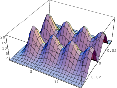
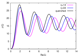
Figure 1: The spectral density with $N_{f}\!=\!2$ eq. (9) at $\alpha\!=\!0.012$, $\eta\!=\!8.74$ and $\nu\!=\!0$ (left), and a cut parallel to the $x$-axis for different masses (right).

containing $K$- and $J$-Bessel functions. The weight for the eigenvalues is non-Gaussian due to the non-trivial decoupling of eigenvectors. The unquenched density

$$\rho^{(N_{f}=2)}(\xi) = \rho^{(0)}(\xi)-(\xi^{\ast\,2}-\xi^{2})w(\xi,\xi^{*})$$ (9)

$$\times\frac{|\kappa(\xi,i\eta)|^{2}-|\kappa(\xi^{*},i\eta)|^{2}}{\kappa(i\eta,i\eta)},$$

with a mass dependent correction term is shown in Fig. 1 left (for more details, see A05 ). Compared to $\mu\!=\!0$ in BMW the peaks locating the eigenvalues are split in two, the particularity of this $\chi$SB class. A cut parallel to the $x$-axis along the maxima illustrates the effect of dynamical flavours at increasing $\eta$. At value $\eta\approx 100$ the smallest eigenvalues are effectively quenched, following eq. (6).

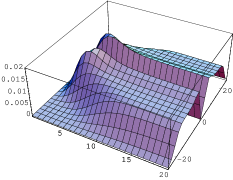
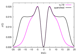
Figure 2: The density eq. (9) at $\alpha\!=\!3.28$, $\eta\!=\!19$, and $\nu\!=\!0$ (left), and a cut parallel to the $y$-axis (right) vs. quenched.

Increasing $\alpha$ rapidly damps the oscillations. In Fig. 2 the density is now constant along a stripe, as expected from mean field. The effect of the additional zeros of $\rho^{(N_{f}=2)}(\xi)$ at $\xi\!=\!\pm i\eta$ in the left corners of Fig. 2 are clearly visible. Here we choose a cut in $y$-direction on the maxima to highlight the difference to quenched. At this value of $\alpha$ the perpendicular cut in $x$-direction shows no dependence on $\eta$, in contrast to the previous figure. In the strong non-Hermiticity limit $\alpha\to\infty$ the plateau extends to $\infty$ in both $x$- and $y$-direction A05 . Away from the edge Fig. 2 is already very close to $\alpha\!=\!\infty$, to which we compared our preliminary data ABLMP .

Table 1: Summary of simulation parameters at $\beta=1.3$

$V$	$\mu$	mass $ma$	level spacing $d$	$\eta$	$\alpha$	$F_{\pi}^{2}/\Sigma$	$E_{Th}$	no. of config.
$6^{4}$	$1.0\cdot 10^{-3}$	$0.035$	$8.0(2)\cdot 10^{-3}$	$13.7$	$0.0124(3)$	$0.39(3)$	$\sim 17$	$45\,000$
$6^{4}$	$1.0\cdot 10^{-3}$	$0.07$	$6.6(2)\cdot 10^{-3}$	$33.3$	$0.0127(3)$	$0.34(3)$	$\sim 25$	$15\,000$
$6^{4}$	$1.0\cdot 10^{-3}$	$20$	$5.0(2)\cdot 10^{-3}$	$12\,566$	$0.0153(3)$	$0.37(3)$	$>100$	$10\,000$
$6^{4}$	$0.2$	$0.06$	$9.9(1)\cdot 10^{-3}$	$19.0$	$2.21(4)$	$0.38(1)$	$\sim 10$	$20\,000$
$6^{4}$	$0.2$	$20$	$4.5(1)\cdot 10^{-3}$	$13\,962$	$3.28(4)$	$0.38(2)$	$>200$	$20\,000$
$8^{4}$	$5.625\cdot 10^{-4}$	$0.035$	$3.0(3)\cdot 10^{-3}$	$35.5$	$0.0107(9)$	$0.35(5)$	$\sim 20$	$8\,000$
$8^{4}$	$5.625\cdot 10^{-4}$	$0.07$	$2.1(1)\cdot 10^{-3}$	$104.7$	$0.0124(3)$	$0.32(4)$	$\sim 35$	$5\,000$
$8^{4}$	$5.625\cdot 10^{-4}$	$20$	$1.6(1)\cdot 10^{-3}$	$39\,270$	$0.0152(3)$	$0.37(4)$	$>35$	$3\,000$
$8^{4}$	$0.1125$	$20$	$1.4(1)\cdot 10^{-3}$	$44\,880$	$3.29(4)$	$0.38(5)$	$>40$	$6\,000$

We now turn to the LGT side, describing the details of our simulations summarised in Table 1. Our data were generated for gauge group $SU(2)$ with $N_{f}\!=\!2$ unimproved staggered fermion flavours of equal mass at coupling constant $\beta\!=\!4/g^{2}\!=\!1.3$, using the code of HKLM . In this setup the fermion determinant remains real and standard Monte Carlo applies. Our choice of parameters was dictated by several constraints: i) Wilson fermions explicitly break chiral symmetry and are already complex at $\mu\!=\!0$, making the effect of $\mu\neq 0$ difficult to disentangle. At $\mu\!=\!0$ Ginsparg-Wilson type fermions have been shown to exactly preserve chiral symmetry and topology (see EHKN for references and a comparison to MM). Similar results have been obtained with improved staggered fermions for QCD EF . Apart from being very expensive it is conceptually not clear so far how to extend these results to $\mu\neq 0$. Thus we use the Dirac operator of standard, unimproved staggered fermions:

$$D_{x,y}=\frac{1}{2a}\Big{[}\sum\limits_{\gamma=\hat{x},\hat{y},\hat{z}}\left(U_{\gamma}(x)\kappa_{\gamma}(x)\delta_{y,x\!+\!\gamma}-{\rm h.c.}\right)$$ (10)

$$+\!\!\left(U_{\hat{t}}(x)\kappa_{\hat{t}}(x)e^{\mu}\delta_{y,x\!+\!\hat{t}}\!-\!U_{\hat{t}}^{\dagger}(y)\kappa_{\hat{t}}(y)e^{-\mu}\delta_{y,x\!-\!\hat{t}}\right)\!\!\Big{]},$$

with link variables $U$ and staggered phases $\kappa$. Consequently our simulations are topology blind, and we set $\nu\!=\!0$ in the following. We note that even at $\mu\!=\!0$ the transition from staggered to the correct continuum symmetry class has not yet been observed. ii) A proper resolution of complex eigenvalues requires of the order of $10^{4}$ configurations for each parameter set. Even with cheap staggered fermions we are confined to small lattices $V\!=6^{4}$ and $8^{4}$. iii) We want to make the window where MM apply as large as possible. At the Thouless energy scale OV , $E_{Th}\sim F_{\pi}^{2}/\Sigma\sqrt{V}$, the Dirac eigenvalues start to feel the propagating Goldstone modes, and leave the $\epsilon$-regime. Increasing $\beta$ (decreasing $F_{\pi}$) at fixed $V$ fewer Dirac eigenvalues follow MM statistics. This leads us to rather strong coupling. iv) Small masses $m$ considerably slow down the computation. Because of rescaling $\eta\!=\!m\Sigma V$ this effects our choice of the volume too.

To compare our data with the prediction eq. (9) we have to determine two parameters from the data. First, we measure the mean level-spacing $d\sim 1/\rho(0)$, by using the Banks-Casher relation at $\mu\!=\!0$, $\pi\rho(0)\!=\!\Sigma V$, where $\rho(0)$ is the mean spectral density. We project the complex eigenvalues onto the real axis and measure their distance. Due to $\mu\ll 1$ the 2d geometric distance between eigenvalues agrees within errors. This provides the volume rescaling of lattice eigenvalues, masses and $\mu^{2}$:

$$za\cdot\pi/d\ \equiv\xi\ ,\ \ ma\cdot\pi/d\ \equiv\eta\ ,\ \ \mbox{and}\ \ \mu^{2}C\cdot\pi/d\equiv\alpha^{2}.$$ (11)

Second, the remaining constant $C\sim F_{\pi}^{2}/\Sigma$ is obtained by a fit to the data. We cut the data rescaled as in eq. (11) parallel to the $y$-axis on the first maxima, which are easy to identify for all $\alpha$. Then we fit to the integral of the analytic curve, thus eliminating the choice of bins in this direction (for clarity we show histograms in all Figures). This procedure avoids cumbersome 3d fits and fixes the normalisation of the first maxima.

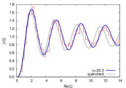
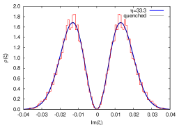
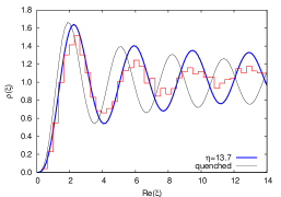
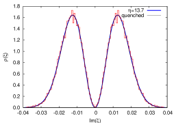
Figure 3: The effect of dynamical fermions at $\mu\!=\!10^{-3}$, $V\!=\!6^{4}$: $\alpha\!=\!0.0127$, $\eta\!=\!33.3$ (upper), and $\alpha\!=\!0.0124$, $\eta\!=\!13.7$ (lower).

We start with $\alpha\ll 1$. For mass $\eta\!=\!33.3$ in Fig. 3 (up) the data show an excellent match to the prediction eq. (9) including the 4$th$ maximum, clearly deviating from the quenched curve shown for comparison. The perpendicular cut on the first maxima (up right) is perfectly agreeing, allowing to fit $\alpha$ to an relative error of $\approx 2\%$. The repulsion from the $x-$axis correctly identifies this $\chi$SB class (QCD has a single peak, see AW ), and we have observed this pattern down to $\mu\!=\!10^{-6}$. Note that fitting $\alpha$ does not move the maxima in the left curves. A similar data set for $V\!=\!8^{4}$ leads to the same conclusions (see Table 1).

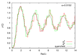
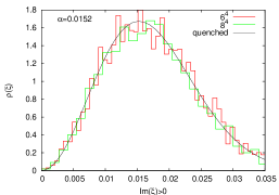
Figure 4: The scaling $\mu_{i}^{2}V_{i}\!=$const.: $V_{1}\!=\!6^{4}$, $\mu_{1}\!=\!10^{-3}$ (green) vs. $V_{2}\!=\!8^{4}$, $\mu_{2}\!=\!5,625\cdot 10^{-4}$ (red), both at $ma\!=\!20$ for $y>0$.

Fig. 3 (down) shows the smallest mass we could simulate, with $\eta\!=\!13.7$. The data follow the analytic curve including the 2$nd$ minimum, deviating substantially from quenched. The onset of $E_{Th}\!\sim\!17$ is responsible for a smaller window of agreement ($E_{Th}\!\sim\!25$ at $\eta\!=\!33.3$). The perpendicular cut shows again perfect agreement. Despite excessive statistics the fluctuations on the maxima are still visible. To exclude that the observed deviations from quenched are finite volume effects we compare to BMW at $\mu\!=\!0$ and otherwise identical parameters. There finite volume shifts the data to the left of the MM curve. Thus for larger volumes the deviation from quenched would be even more pronounced.

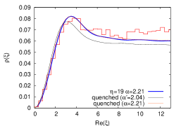
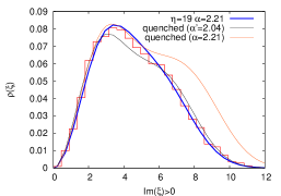
Figure 5: The effect of dynamical fermions at $\mu\!=\!0.2$, $V\!=\!6^{4}$: $\alpha\!=\!2.21$, $\eta\!=\!19.0$ for $y>0$. Note that $E_{Th}\!\sim\!10$.

Second we check the scaling hypothesis from MM and $\epsilon\chi$PT, choosing $\mu_{1}^{2}/\mu_{2}^{2}\!=\!6^{4}/8^{4}$ with $\mu_{i}^{2}V_{i}\!=$ const. For simplicity footnote1 we have chosen a large $\eta$ to effectively quench the small eigenvalues. In Fig. 4 both sets of data show an excellent agreement to the same curve from eq. (6). Independent fits for $\alpha$ agree within errorbars. Here only $y\!>\!0$ is shown for a better resolution, the second peak at $y\!<\!0$ follows from symmetry. The same results are obtained for smaller, unquenched masses (see Table 1).

Next we turn to a larger $\mu$, remaining below the phase transition $\mu_{c}\approx 0.3$ found in BLMP for $V\!=\!6^{4}$, $\beta\!=\!1.3$. Above the transition at $\mu\!=\!0.4$ the data deviate from the MM as expected. We first determine $d$, which fixes the scale and $\eta$. At these parameter values unquenching is seen in $y$-direction (Fig. 5 right), which is used to fit $\alpha$. Here both $\alpha$ and the given $\eta$ influence the width. We therefore compare the unquenched curve to the quenched one with $\alpha^{\prime}\neq\alpha$ fitted independently (lower curve). For comparison we also give the quenched curve at the same $\alpha$ (upper curve). Again we display $y>0$ only. Clearly the unquenched curve describes the data best both in $x$- and $y$-direction. The onset of $E_{Th}$ is responsible for the deviation between data and MM for $x>10$ in Fig. 5 (left). In Fig. 6 the scaling of constant $\mu_{i}^{2}V_{i}$ is tested for these $\mu$-values, where we have again chosen $\eta_{i}\gg 100$ to effectively quench. Both data sets nicely follow the same curve, the fits for $\alpha$ agree within errorbars.

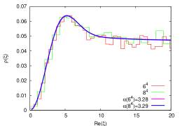
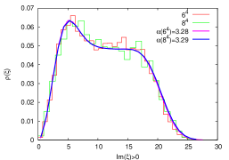
Figure 6: The scaling of $\mu_{i}^{2}V_{i}\!=$const.: $V_{1}\!=\!6^{4}$, $\mu_{1}\!=\!0.2$ (red) vs. $V_{2}\!=\!8^{4}$, $\mu_{2}\!=\!0.1125$ (green), both at $ma\!=\!20$ for $y>0$.

To conclude we have shown that our unquenched $SU(2)$ lattice data are quantitatively very well described by complex MM predictions over a wide range of chemical potentials and masses. We find agreement with $\epsilon\chi$PT by confirming the scaling $F_{\pi}^{2}V\mu^{2}$, with a consistent value for $F_{\pi}^{2}/\Sigma\sim 0.37$ for all our data. This further indicates a MM–$\epsilon\chi$PT equivalence for $SU(2)$ at $\mu\neq 0$.

We thank P. Damgaard, M.-P. Lombardo, H. Markum, J.C. Osborn, K. Splittorff, J.J.M. Verbaarschot and T. Wettig for useful conversation. This work was supported by BRIEF award 707, EU network ENRAGE MRTN-CT-2004-005616, EPSRC grant EP/D031613/1 (G.A.), and DFG grant JA483/22-1 (E.B.).

References

- (1) For a review and references: Y.V. Fyodorov, H.-J. Sommers, J. Phys. A: Math. Gen. 36 (2003) 3303.
- (2) R. Grobe, F. Haake, H.-J. Sommers, Phys. Rev. Lett. 61 (1988) 1899
- (3) K.B. Efetov, Phys. Rev. Lett. 79 (1997) 491.
- (4) M. Stephanov, Phys. Rev. Lett. 76 (1996) 4472.
- (5) For a recent review: V. Azcoiti, A. Galante, V. Laliena, Prog. Theor. Phys. 109 (2003) 843.
- (6) J.C. Osborn, K. Splittorff, J.J.M. Verbaarschot, Phys. Rev. Lett. 94 (2005) 202001
- (7) J.C. Osborn, Phys. Rev. Lett. 93 (2004) 222001; G. Akemann et al. Nucl. Phys. B712 (2005) 287.
- (8) S. Muroya et al., Prog. Theor. Phys. 110 (2003) 615.
- (9) K. Splittorff, J.J.M. Verbaarschot, Nucl. Phys. B683 (2004) 467.
- (10) G. Akemann, Y.V. Fyodorov, G. Vernizzi, Nucl. Phys. B694 (2004) 59.
- (11) M.A. Halasz, J.C. Osborn, J.J.M. Verbaarschot, Phys. Rev. D56 (1997) 7059.
- (12) S. Hands et al., Nucl. Phys. B558 (1999) 327.
- (13) G. Akemann, Nucl. Phys. B730 (2005) 253.
- (14) G. Akemann et al., Nucl. Phys. B140 Proc. Suppl. (2005) 568, G. Akemann, E. Bittner, PoS LAT2005 (2005) 197.
- (15) M.E. Berbenni-Bitsch, S. Meyer, T. Wettig, Phys. Rev. D58 (1998) 071502, G. Akemann, E. Kanzieper, Phys. Rev. Lett. 85 (2000) 1174.
- (16) G. Akemann, T. Wettig, Phys. Rev. Lett. 92 (2004) 102002; Erratum-ibid. 96 (2006) 029902.
- (17) J.C. Osborn, T. Wettig, PoS LAT2005 (2005) 200.
- (18) J. B. Kogut et al., Nucl. Phys. B582 (2000) 477.
- (19) P.H. Damgaard et al., Phys. Rev. D72 (2005) 091501.
- (20) R.G. Edwards et al., Phys. Rev. Lett. 82 (1999) 4188.
- (21) E. Follana, Nucl. Phys. B140 Proc. Suppl. (2005) 141.
- (22) J.C. Osborn, J.J.M. Verbaarschot, Phys. Rev. Lett. 81 (1998) 268.
- (23) Keeping and mass const. results into different spacings and for with the same . In Fig. 4 both lead to the same quenched curve.
- (24) E. Bittner et al., Nucl. Phys. B106 Proc. Suppl. (2002) 468.