Relation between bare lattice coupling and $\overline{MS}$ coupling at one loop with general lattice fermions

David H. Adams dadams@phya.snu.ac.kr Dept. of Physics and Astronomy, Seoul National University, Seoul, 151-747, South Korea Current address Physics Dept., National Taiwan University, Taipei 106, Taiwan R.O.C. Physics Dept., Florida International University, 11200 SW 8th St., Miami, FL 33199, U.S.A.
(April 26, 2008)
Abstract

A compact general integral formula is derived from which the fermionic contribution to the one-loop coefficient in the perturbative expansion of the $\overline{MS}$ coupling in powers of the bare lattice coupling can be extracted. It is seen to reproduce the known results for unimproved naive, staggered and Wilson fermions, and has advantageous features which facilitate the evaluation in the case of improved lattice fermion formulations. This is illustrated in the case of Wilson clover fermions, and an expression in terms of known lattice integrals is obtained in this case which gives the coefficient to much greater numerical accuracy than in the previous literature.

pacs:
11.15.Ha, 11.25.Db

I Introduction

When transforming results from lattice simulations into a continuum scheme such as $\overline{MS}$ it is often desirable to know the perturbative expansion of the renormalized coupling in powers of the bare lattice coupling. This is useful as an intermediate step for relating the $\overline{MS}$ coupling to the coupling defined in nonperturbative lattice schemes such as the ones based on the static quark potential Lepage-Mackenzie ; Trottier(review) and SchrΓΆdinger functional L-W(Schrodinger) ; Bode-Weisz , and is also needed to translate bare lattice quark masses into the $\overline{MS}$ scheme (see, e.g., Sachrajda ; staggeredmass ). The one loop coefficient in the expansion is of further interest because it determines the ratio of the lattice and $\overline{MS}$ $\Lambda$-parameters Has(L)(PLB) ; DashenGross ; Has(L)(NPB) ; Kawai ; Weisz(PLB) ; Weisz(NPB) ; Vicari ; Skour-Pan . Moreover, the one loop coefficient is also needed for determining the two loop relation between the couplings, from which the third term in the lattice beta-function (governing the approach to the continuum limit) can be determined L-W(Schrodinger) ; Alles ; Christou ; Bode-Pan ; Const-Pan1 ; Const-Pan2 .

In this paper we derive, for general lattice fermion formulation, a compact general integral formula from which the fermionic contribution to the one-loop coefficient in the perturbative expansion of the $\overline{MS}$ coupling in powers of the bare lattice coupling can be extracted. The motivations for pursuing this are as follows. First, given the plethora of lattice fermion actions currently in use, and the likelyhood of new ones or improved versions of present ones being developed in the future, it is desirable where possible to have general formulae from which quantities of interest can be calculated without having to do the calculation from scratch each time. Second, it is desirable to have independent ways to check the computer programs used these days to perform lattice perturbation theory calculations via symbolic manipulations. Third, by reducing the calculation to a managable number of one loop lattice integrals one can more easily achieve greater numerical precision than with symbolic computer programs. This is important, since, as emphasized in Capitani , the one loop results need to be determined with very high precision to achieve reasonable precision in the two loop result. As a demonstration that the general formulae of this paper are useful in this regard, we apply them to obtain the fermionic contribution to the one loop coefficient in the case of Wilson clover fermions clover to almost twice as many significant decimal places as in the previous literature.

As reviewed in sect. II, determining the fermionic contribution to the one loop coefficient reduces to determining a constant $c_{I}$ arising in a logarithmically divergent one fermion loop lattice Feynman integral $I(am)$, which has the general structure

$\displaystyle I(am)=\frac{1}{24\pi^{2}}\log(a^{2}m^{2})+c_{I}$ (1)

Here $a$ is the lattice spacing and $m$ an infrared regulator fermion mass. The numerical factor in the log term is universal, whereas $c_{I}$ depends on the details of the lattice fermion formulation. $I(am)$ arises from the one fermion loop contribution to the gluonic 2-point function, and it is from this that it was evaluated in previous works for specific lattice fermion formulations. However, Ward Identities allow $I(am)$ to also be evaluated from the gluonic 3- or 4-point functions. In this paper we evaluate $I(am)$ from the one fermion loop contribution to the gluonic 4-point function. In this case there are five lattice Feynman diagrams to consider rather than the two diagrams for the gluonic 2-point function – see Fig. 1.
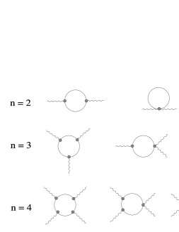
Refer to caption
Figure 1: The lattice Feynman diagrams for the gluonic $n$-point function with internal fermion loop for $n\!=\!2,3,4$.

Nevertheless, evaluation of $I(am)$ from the 4-point function turns out to be advantageous. The diagrams are evaluated at vanishing external momenta without the need to first take momentum derivatives, and we find three nice properties: (i) Only one of the five diagrams is logarithmically divergent – it is the first $n\!=\!4$ diagram in Fig. 1. The other four diagrams are all convergent. (ii) The logarithmically divergent diagram is not affected by changes in how the link variables are coupled to the fermions (e.g., it is unchanged by adding staples, clover term etc.). Consequently, it is the same for improved and unimproved versions of the lattice fermion formulation (provided the free field formulations are the same). (iii) The four convergent diagrams, or subsets of them, vanish when the lattice Dirac operator is sufficiently simple. In particular, they all vanish for unimproved Wilson and staggered fermions, also when the Naik term Naik is included. Thus for improved versions of Wilson and staggered fermions the only new quantities to compute relative to the unimproved case are the four convergent one-loop lattice integrals.111This is only true in the staggered fermion case when the Naik term is not used. More on this in the concluding section.

The main result in this paper is a general integral formula for $I(am)$ obtained by evaluating the contributions from the five $n\!=\!4$ Feynman diagrams in Fig. 1 for general lattice fermion formulation, from which the desired constant $c_{I}$ can be extracted. Specifically, we do the following: (a) evaluate the contribution from the logarithmically divergent diagram, deriving a quite explicit general formula which is seen to reproduce previous results for the cases of unimproved Wilson and naive/staggered fermions, and (b) derive formulae for, and describe a straightforward procedure for evaluating, the contributions from the four convergent diagrams. We illustrate this in the case of Wilson clover fermions. The general formulae lead to integrals to which the method of Ref. Burgio can be applied, reducing the integrals to basic lattice integrals that are already known to high precision. The application of our result to other lattice fermion formulations such as Asqtad staggered fermions asqtad and overlap fermions overlap will be made in future work.

The paper is organized as follows. Sect. II reviews the one loop expansion of the $\overline{MS}$ coupling in the bare lattice coupling, using the background field approach. In sect. III we derive an initial expression for $I(am)$ as the sum of contributions from the five $n\!=\!4$ diagrams in Fig. 1 and point out the properties (i), (ii) and (iii) mentioned above. Rather than evaluating the diagrams directly, we infer them from perturbative expansion of the fermion determinant, which is easier. From this the general formulae and applications mentioned in (a) and (b) above are derived in sect. IV and V, respectively. The concluding sect. VI describes applications to be carried out in future work, as well as the possibility of deriving similar results for the gauge–ghost contribution to the one loop coefficient. Also, it is pointed out that the present results are relevant for a previous proposal for constructing the gauge field action on the lattice from the lattice fermion determinant Horvath . Specifically, our results give an expression for the coefficient of the Yang-Mills action that arises in that proposal. Some technical details of our calculations are provided in two appendices.

II Generalities of the one-loop relation betwen bare lattice coupling and $\overline{MS}$ coupling

The gauge field quantum effective action $\Gamma(A)$ in Euclidean spacetime can be expressed (prior to gauge fixing) as

$\displaystyle e^{-\Gamma(A)}=\int{\cal D}Q{\cal D}\bar{\psi}{\cal D}\psi\,e^{-\frac{1}{g^{2}}S_{YM}(A+gQ)-\int\bar{\psi}D(A+gQ)\psi}$ (2)

where $S_{YM}$ is the Yang-Mills action and $D(A+gQ)$ is the Dirac operator coupled to $A+gQ$ where $A$ is the background gauge field and $Q$ the quantum fluctuation field. The gauge group is taken to be SU(N) with the fermion fields being in the fundamental representation. $\Gamma(A)$ has the loop expansion

$\displaystyle\Gamma(A)=\frac{1}{g^{2}}S_{YM}(A)+\Gamma_{1}(A)+g^{2}\Gamma_{2}(A)+\dots+g^{2(n-1)}\Gamma_{n}(A)+\dots$ (3)

Expanding $\Gamma(A)$ in powers of $A$, the term quadratic in $A$ has the form

$\displaystyle\Gamma^{(2)}(A)=\int_{p}\Gamma^{(2)}(p)_{\mu\nu}^{ab}\,\hat{A}_{\mu}^{a}(p)\hat{A}_{\nu}^{b}(-p)$ (4)

where $\hat{A}_{\mu}^{a}(p)$ denotes the Fourier transform of $A_{\mu}^{a}(x)$. Gauge invariance of $\Gamma(A)$ and rotation symmetry imply that the 2-point function has the form

$\displaystyle\Gamma^{(2)}(p)_{\mu\nu}^{ab}=-\delta^{ab}(p^{2}\delta_{\mu\nu}-p_{\mu}p_{\nu})\Big{[}\frac{1}{g^{2}}-\nu_{1}(p)-\dots-g^{2(n-1)}\nu_{n}(p)-\dots\Big{]}$ (5)

The relation between the $\overline{MS}$ renormalized coupling $g$ and bare lattice coupling $g_{0}$ at one loop can be obtained by requiring equality of $\Gamma(A)_{\overline{MS}}$ and $\Gamma(A)_{lat}$ up to one loop DashenGross ; Has(L)(NPB) :

$\displaystyle\frac{1}{g^{2}}S_{YM}(A)+\Gamma_{1}(A)_{\overline{MS}}=\frac{1}{g_{0}^{2}}S_{YM}(A)+\Gamma_{1}(A)_{lat}$ (6)

Expanding each side in powers of $A$, the equality betwen the quadratic terms gives, in light of (5),222In the lattice theory there is only hypercubic rotation symmetry. However, this suffices to obtain (5) in the lattice setting up to terms which vanish for $a\to 0$.

$\displaystyle\frac{1}{g^{2}}-\nu_{1}(p)_{\overline{MS}}=\frac{1}{g_{0}^{2}}-\nu_{1}(p)_{lat}$ (7)

The one-loop contribution to the 2-point function is given by a sum of 3 terms: gauge field loop, ghost loop and fermion loop. Consequently, for $N_{f}$ flavors of massless fermions, $\nu_{1}(p)_{\overline{MS}}$ and $\nu_{1}(p)_{lat}$ have the general forms

$\displaystyle\nu_{1}(p)_{\overline{MS}}$ $\displaystyle=$ $\displaystyle-\beta_{0}\log(p^{2}/\mu^{2})+c_{\overline{MS}}^{g}+N_{f}\,c_{\overline{MS}}^{f}$ (8)
$\displaystyle\nu_{1}(p)_{lat}$ $\displaystyle=$ $\displaystyle-\beta_{0}\log(a^{2}p^{2})+c_{lat}^{g}+N_{f}\,c_{lat}^{f}$ (9)

where $\mu$ is the mass scale in the $\overline{MS}$ scheme, $a$ is the lattice spacing, and

$\displaystyle\beta_{0}=\frac{1}{16\pi^{2}}\Big{(}N\frac{11}{3}-N_{f}\frac{2}{3}\Big{)}$ (10)

The constant $c^{g}$ arises from the gauge and ghost loop contributions; it depends on $N$ and the gauge fixing parameter, while $c^{f}$ arises from the fermion loop contribution. In the lattice case $c^{g}$ and $c^{f}$ also depend on whatever parameters are present in the lattice gauge and fermion actions. (E.g., for lattice Wilson fermions $c_{lat}^{f}$ depends on the Wilson parameter.)

From (7) and (8)–(9) we get

$\displaystyle\frac{1}{g^{2}}=\frac{1}{g_{0}^{2}}+\beta_{0}\log(a^{2}\mu^{2})+l_{0}$ (11)

where

$\displaystyle l_{0}$ $\displaystyle=$ $\displaystyle l_{0}^{g}+N_{f}l_{0}^{f}$ (12)
$\displaystyle l_{0}^{g}=c_{\overline{MS}}^{g}-c_{lat}^{g}$ , $\displaystyle\qquad l_{0}^{f}=c_{\overline{MS}}^{f}-c_{lat}^{f}$ (13)

(Our notations $l_{0}\,$, $l_{0}^{g}\,$, $l_{0}^{f}$ follow the papers of Panagopoulos and collaborators, e.g., Skour-Pan ) The relation bewteen $g$ and $g_{0}$ up to one loop now follows from (11):

$\displaystyle g^{2}=g_{0}^{2}(1-g_{0}^{2}[\beta_{0}\log(a^{2}\mu^{2})+l_{0}]+O(g_{0}^{4})\,)$ (14)

Also, from (11) or (14) the relation between the lattice and $\overline{MS}$ $\Lambda$-parameters is obtained Has(L)(PLB) ; DashenGross ; Has(L)(NPB) ; Kawai ; Weisz(PLB) :

$\displaystyle\frac{\Lambda_{lat}}{\Lambda_{\overline{MS}}}=e^{l_{0}/2\beta_{0}}$ (15)

The focus of our attention in this paper is the fermionic contribution to $l_{0}\,$, i.e., $l_{0}^{f}$ in (13) for general lattice fermion formulation. The continuum constant $c_{\overline{MS}}^{f}$ is well-known (see, e.g., Christou ):

$\displaystyle c_{\overline{MS}}^{f}=-\frac{5}{72\pi^{2}}$ (16)

Therefore, to determine $l_{0}^{f}$ we need to determine the lattice constant $c_{lat}^{f}$ for general lattice fermion formulation.

To study $c_{lat}^{f}$ it suffices to consider the $N_{f}=1$ case which we restrict to henceforth. We proceed by expanding the lattice 2-point function $\Gamma_{lat}^{(2)}(p)_{\mu\nu}^{ab}$ in powers of (the components of) the external momentum $p$. Although $\Gamma_{lat}^{(2)}(p)_{\mu\nu}^{ab}$ itself is infrared finite, the terms in the expansion are individually infrared divergent. To deal with this we introduce a fermion mass $m$ as regulator; it renders the expansion terms finite. Since gauge invariance is maintained when $m$ is introduced, the expansion of the one fermion loop contribution to $\Gamma_{lat}^{(2)}(p)_{\mu\nu}^{ab}$ up to 2nd order in $p$ results in an expression of the general form

$\displaystyle\Big{[}\Gamma_{lat}^{(2)}(p)_{\mu\nu}^{ab}\Big{]}_{f,\,1-loop}=\delta^{ab}(p^{2}\delta_{\mu\nu}-p_{\mu}p_{\nu})[I(am)+R(p^{2}/m^{2})]$ (17)

up to terms which vanish for lattice spacing $a\to 0$. Here $I(am)$ is a logarithmically divergent one loop lattice Feynman integral given by

I​(a​m)=βˆ’βˆ‚ΞΌβˆ‚Ξ½[Ξ“l​a​t(2)​(p)μ​ν11]f, 1βˆ’l​o​o​p|p=0(ΞΌβ‰ Ξ½, no sum)πΌπ‘Žπ‘ševaluated-atsubscriptπœ‡subscript𝜈subscriptdelimited-[]superscriptsubscriptΞ“π‘™π‘Žπ‘‘2superscriptsubscriptπ‘πœ‡πœˆ11𝑓1π‘™π‘œπ‘œπ‘π‘0(ΞΌβ‰ Ξ½, no sum)\displaystyle I(am)=-\partial_{\mu}\partial_{\nu}\Big{[}\Gamma_{lat}^{(2)}(p)_{\mu\nu}^{11}\Big{]}_{f,\,1-loop}\Big{|}_{p=0}\quad\quad\mbox{($\mu\neq\nu\,,\ $ no sum)} (18)

($\partial_{\mu}\equiv\frac{\partial}{\partial p_{\mu}}$). By the structural result of DA(logdiv) it has the general form333The factor $1/24\pi^{2}$ in the log term is fixed by universality DA(logdiv) ; it is minus the fermionic term in $\beta_{0}$ with $N_{f}\!=\!1$.

$\displaystyle I(am)=\frac{1}{24\pi^{2}}\log(a^{2}m^{2})+c_{I}$ (19)

where the constant $c_{I}$ depends on the details of the lattice fermion formulation. $R(p^{2}/m^{2})$ in (17) denotes the continuum limit of the remainder term after expanding $[\Gamma_{lat}^{(2)}(p)_{\mu\nu}^{ab}]_{f,\,1-loop}$ to 2nd order in $p$. It is convergent by power-counting and therefore coincides Reisz(CMP) with the corresponding (known) continuum term:

$\displaystyle R(p^{2}/m^{2})$ $\displaystyle=$ $\displaystyle\frac{1}{4\pi^{2}}\int_{0}^{1}dx\,x(1-x)\log\Big{[}x(1-x)\frac{p^{2}}{m^{2}}+1\Big{]}$ (20)
$\displaystyle=$ $\displaystyle\frac{1}{24\pi^{2}}\log(p^{2}/m^{2})+\frac{1}{4\pi^{2}}\int_{0}^{1}dx\,x(1-x)\log\Big{[}x(1-x)+\frac{m^{2}}{p^{2}}\Big{]}$
$\displaystyle\equiv$ $\displaystyle\frac{1}{24\pi^{2}}\log(p^{2}/m^{2})+\widetilde{R}(m^{2}/p^{2})$

Substituting (19) and (20) in (17) gives

$\displaystyle\Big{[}\Gamma_{lat}^{(2)}(p)_{\mu\nu}^{ab}\Big{]}_{f,\,1-loop}=\delta^{ab}(p^{2}\delta_{\mu\nu}-p_{\mu}p_{\nu})\Big{[}\frac{1}{24\pi^{2}}\log(a^{2}p^{2})+c_{I}+\widetilde{R}(m^{2}/p^{2})\Big{]}$ (21)

Comparing this to the expression (5) for $\Gamma_{lat}^{(2)}(p)_{\mu\nu}^{ab}$ with $\nu_{1}(p)_{lat}$ given by (9), we see that

$\displaystyle c_{lat}^{f}=c_{I}+\widetilde{R}(0)$ (22)

In fact $\widetilde{R}(0)$ is precisely the $\overline{MS}$ constant $c_{\overline{MS}}^{f}\,$: explicit evaluation of the integral in (20) at $m=0$ gives $\widetilde{R}(0)=-5/72\pi^{2}$. It follows from (13) that

$\displaystyle l_{0}^{f}=-c_{I}$ (23)

Thus the issue is to determine the constant $c_{I}$ appearing in the logarithmically divergent one-loop lattice integral $I(am)$ in (18)–(19). In this paper we are going to derive a compact general formula for $I(am)$ for general lattice fermions which can then be used to determine $c_{I}$.

III An initial formula for $I(am)$

In this section we derive an initial general formula for $I(am)$. It is the starting point for deriving more explicit formulae in the subsequent sections.

Let $D$ be a general lattice Dirac operator which is translation-invariant and transforms covariantly under gauge transformations and rotations of the 4-dimensional Euclidean hypercubic lattice. The ansatz for the link variables is

$\displaystyle U_{\mu}(x)=e^{aA_{\mu}(x+\frac{1}{2}a\hat{\mu})}$ (24)

($\hat{\mu}$=unit vector in the positive $\mu$-direction). The Fourier-transformed field $\hat{A}_{\mu}(p)$ is defined via

$\displaystyle A_{\mu}(x+\frac{1}{2}a\hat{\mu})=\int_{p}\,\hat{A}_{\mu}(p)\,e^{ip\cdot(x+\frac{1}{2}a\hat{\mu})}\,.$ (25)

Here and in the following $\int_{p}(\cdots)\equiv\int_{-\pi/a}^{\pi/a}\,\frac{d^{4}p}{(2\pi)^{4}}\,(\cdots)\,$. The continuum gauge fields are $A_{\mu}(x)=A_{\mu}^{a}(x)T^{a}$ where $\{T^{a}\}$ are generators for SU(N) normalized such that $tr(T^{a}T^{b})=-\frac{1}{2}\delta^{ab}$. (We take the $T^{a}$’s to be anti-hermitian, absorbing into them the imaginary unit that multiplies $A$ in other notations.)

Expanding the link variables in powers of $A$ gives an expansion of the lattice Dirac operator,

$\displaystyle D=\sum_{n=0}^{\infty}D_{n}$ (26)

Translation-invariance implies that each $D_{n}$ can be expressed in momentum basis in the form

$\displaystyle D_{n}(k^{\prime},k)$ $\displaystyle=$ $\displaystyle a^{n-1}\int_{p_{1},\dots,p_{n}}\,\delta(p_{1}+\dots+p_{n}+k-k^{\prime})\,d_{n}(ak\,|\,ap_{1},\dots,ap_{n})_{\mu_{1}\cdots\mu_{n}}\hat{A}_{\mu_{1}}(p_{1})\cdots\hat{A}_{\mu_{n}}(p_{n})$

The continuum limit requirements on $D$ are

$\displaystyle\frac{1}{a}\,d_{0}(ak)$ $\displaystyle\stackrel{{\scriptstyle a\to 0}}{{\longrightarrow}}$ $\displaystyle i\gamma_{\nu}k_{\nu}+m$ (28)
$\displaystyle d_{1}(ak\,|\,ap)_{\mu}$ $\displaystyle\stackrel{{\scriptstyle a\to 0}}{{\longrightarrow}}$ $\displaystyle\gamma_{\mu}$ (29)

The mass $m$ enters via an additive term $am$ in $d_{0}(ak)$ (we suppress the $m$-dependence in the notation).

To derive a general formula for $I(am)$ it is useful to exploit the fact, clear from (2), that the one fermion loop contribution to $\Gamma(A)$ is given by the fermion determinant:

$\displaystyle\Gamma(A)_{f,\,1-loop}=-\log\det D$ (30)

where, in the present lattice setting, $D$ is coupled to the link variables (24) of the background gauge field $A$. Decomposing $D$ as

$\displaystyle D=D_{0}+D_{int}$ (31)

where $D_{0}$ is the free field operator and $D_{int}$ the interaction part, we start from $D=D_{0}(1+D_{0}^{-1}D_{int})$ to obtain the expansion

$\displaystyle\log\det D-\log\det D_{0}$ $\displaystyle=$ $\displaystyle Tr\,\log(1+D_{0}^{-1}D_{int})$ (32)
$\displaystyle=$ $\displaystyle\sum_{l=1}^{\infty}\frac{(-1)^{l-1}}{l}Tr[(D_{0}^{-1}D_{int})^{l}]$

From this, using $D_{int}=\sum_{n\geq 1}D_{n}$ with $D_{n}$ given by (LABEL:3.4), an expansion in powers of $A$ is obtained. It has the general form

$\displaystyle\log\det D-\log\det D_{0}=\sum_{n\geq 1}\int_{p_{1},\dots,p_{n-1}}\Gamma_{\det}^{(n)}(p_{1},\dots,p_{n-1})_{\mu_{1}\cdots\mu_{n}}tr\hat{A}_{\mu_{1}}(p_{1})\cdots\hat{A}_{\mu_{n}}(p_{n})$ (33)

($p_{n}=-(p_{1}+\dots+p_{n-1})$). The β€œn𝑛n-point function” $\Gamma_{\det}^{(n)}(p_{1},\dots,p_{n-1})_{\mu_{1}\cdots\mu_{n}}$ can be Taylor-expanded in powers of (the components of) $p_{1},\dots,p_{n-1}\,$. Gauge invariance and mass-dimension considerations imply that the terms in the expansion can be combined to take the form444In order for the link variables (24) to transform in the correct way under lattice gauge transformations the transformation of the continuum gauge field $A$ needs to be modified in the lattice setting Kawai ; Reisz(NPB) . However, one still finds that the mass-dimension zero function in (34) must be $\sim S_{YM}(A)$ – this can be inferred from the argument in T. Reisz’s proof of renormalizability of Lattice QCD Reisz(NPB) ; see also Β§5 of Kawai .

$\displaystyle\log\det D-\log\det D_{0}=-I(am)S_{YM}(A)+\sum_{r\geq 1}\frac{1}{m^{r}}S_{r}(A)$ (34)

up to terms which vanish for $a\to 0$, where each $S_{r}(A)$ is a gauge invariant function with mass dimension $r\geq 1$. The fact that the coefficient of $S_{YM}(A)$ is $-I(am)$ is inferred from (17) and (30).

It is clear from (34) and (30) that $I(am)$ can be evaluated from either the 2-, 3- or 4-point function in (33). For the 4-point function the relation is

$\displaystyle I(am)=-\Gamma_{\det}^{(4)}(0,0,0)_{\mu\nu\mu\nu}\qquad\quad\mu\neq\nu\ ,\ \ \mbox{no sum}$ (35)

for any choice of $\mu$ and $\nu$ with ΞΌβ‰ Ξ½πœ‡πœˆ\mu\neq\nu. Usually $I(am)$ is evaluated from the 2-point function via (18), but we will see in the following that it is advantageous to use (35) instead. To evaluate it we start by collecting the terms containing 4 powers of $A$ in the the expansion of $\log\det D$ in (32). These are

$\displaystyle{\textstyle\frac{(-1)^{3}}{4}}\,Tr[(D_{0}^{-1}D_{1})^{4}]\ +\ {\textstyle\frac{(-1)^{2}}{3}}\,3Tr[(D_{0}^{-1}D_{1})^{2}D_{0}^{-1}D_{2}]$
$\displaystyle\quad+\ {\textstyle\frac{(-1)^{1}}{2}}\Big{(}2Tr(D_{0}^{-1}D_{1}D_{0}^{-1}D_{3})\ +\ Tr[(D_{0}^{-1}D_{2})^{2}]\Big{)}\ +\ {\textstyle\frac{(-1)^{0}}{1}}\,Tr(D_{0}^{-1}D_{4})$ (36)

Inserting the expression (LABEL:3.4) for each $D_{n}\,$, and evaluating the traces in momentum basis, the $\Gamma_{\det}^{(4)}(p_{1},p_{2},p_{3})_{\mu_{1}\mu_{2}\mu_{3}\mu_{4}}$ in (32) is readily worked out. The resulting expression for $I(am)$ from (35) is as follows. From the functions $d_{n}$ in (LABEL:3.4) we define

$\displaystyle d_{n}(k)_{\mu_{1}\cdots\mu_{n}}\;\equiv\;d_{n}(k\,|\,0,\dots,0)_{\mu_{1}\cdots\mu_{n}}$ (37)

Then

$\displaystyle I(am)=I_{(1,1,1,1)}(am)+I_{(1,1,2)}(am)+I_{(2,2)}(am)+I_{(1,3)}(am)+I_{(0,4)}(am)$ (38)

where

$\displaystyle I_{(1,1,1,1)}(am)=\frac{1}{4}\int_{-\pi}^{\pi}\frac{d^{4}k}{(2\pi)^{4}}\,tr\,d_{0}(k)^{-1}d_{1}(k)_{\mu}\,d_{0}(k)^{-1}d_{1}(k)_{\nu}\,d_{0}(k)^{-1}d_{1}(k)_{\mu}\,d_{0}(k)^{-1}d_{1}(k)_{\nu}$
(39)
$\displaystyle I_{(1,1,2)}(am)=-\int_{-\pi}^{\pi}\frac{d^{4}k}{(2\pi)^{4}}\,tr\,d_{0}(k)^{-1}d_{1}(k)_{\mu}\,d_{0}(k)^{-1}d_{1}(k)_{\nu}\,d_{0}(k)^{-1}d_{2}(k)_{\mu\nu}$ (40)
$\displaystyle I_{(2,2)}(am)=\frac{1}{2}\int_{-\pi}^{\pi}\frac{d^{4}k}{(2\pi)^{4}}\,tr\,d_{0}(k)^{-1}d_{2}(k)_{\mu\nu}\,d_{0}(k)^{-1}d_{2}(k)_{\mu\nu}$ (41)
$\displaystyle I_{(1,3)}(am)=\int_{-\pi}^{\pi}\frac{d^{4}k}{(2\pi)^{4}}\,tr\,d_{0}(k)^{-1}d_{1}(k)_{\mu}\,d_{0}(k)^{-1}\,d_{3}(k)_{\nu\mu\nu}$ (42)
$\displaystyle I_{(0,4)}(am)=-\int_{-\pi}^{\pi}\frac{d^{4}k}{(2\pi)^{4}}\,tr\,d_{0}(k)^{-1}d_{4}(k)_{\mu\nu\mu\nu}$ (43)

for any choice of $\mu$ and $\nu$ with ΞΌβ‰ Ξ½πœ‡πœˆ\mu\neq\nu (no sum over repeated indices). The traces are over spinor indices alone. Each integral corresponds to an $n\!=\!4$ Feynman diagram in Fig. 1 in sect. I and the notation reflects the structure of the corresponding diagram. The above integrals could have been derived directly from the Feynman diagrams, with fermion propagator and vertices read off from (LABEL:3.4), but it is easier (and equivalent) to use the fermion determinant expansion as we have done above.

The expression of $I(am)$ as the sum of the integrals (39)–(43) is our initial general formula. It has a number of advantageous features which we note in the following.

In light of (28) it is clear that the integral $I_{(1,1,1,1)}(am)$ diverges logarithmically for $am\to 0$ while the other integrals (40)–(43) are all finite in this limit. The divergent integral necessarily DA(logdiv) has the general form

$\displaystyle I_{(1,1,1,1)}(am)=\frac{1}{24\pi^{2}}\log(a^{2}m^{2})+\tilde{c}_{I}$ (44)

up to terms which vanish for $a\to 0$. Then $c_{I}$ is given by

$\displaystyle c_{I}=\tilde{c}_{I}+I_{(1,1,2)}(0)+I_{(2,2)}(0)+I_{(1,3)}(0)+I_{(0,4)}(0)$ (45)

Next we point out that $I_{(1,1,1,1)}(am)$, and hence $\tilde{c}_{I}$, depend only on the free field lattice Dirac operator. This is because $d_{1}(k)_{\mu}$ in (39) is determined by $d_{0}(k)\,$: for any lattice fermion formulation we have

$\displaystyle d_{1}(k)_{\mu}=\frac{1}{i}\,\frac{d}{dk_{\mu}}\,d_{0}(k)\,.$ (46)

This is derived in Appendix A. Therefore, a change of gauging of $D$ (e.g., by adding staples, clover term etc.) affects only the finite integrals (40)–(43).

A further advantage becomes apparent when considering the description of $D$ in terms of lattice paths Has(path) ; Gatt(path) (we will discuss the path description more explicitly in sect. V). It is easy to see that the vertex function $d_{n}(k\,|\,p_{1},\dots,p_{n})_{\mu_{1}\cdots\mu_{n}}$ receives contributions only from lattice paths which contain a lattice link parallel to the $\mu_{1}$-axis, preceded at some point by a link parallel to the $\mu_{2}$-axis, preceded at some point by a link parallel to the $\mu_{3}$-axis, and so on. In particular, if the lattice paths describing $D$ are straight lines, as is the case for the Wilson-Dirac, naive and staggered operators, then $d_{n}(k)_{\mu_{1}\cdots\mu_{n}}$ vanishes unless the $\mu_{j}$’s are all the same. It follows that the finite terms (40)–(43) all vanish in this case (since ΞΌβ‰ Ξ½πœ‡πœˆ\mu\neq\nu there). Thus, for such lattice Dirac operators, $I(am)$ is given entirely by $I_{(1,1,1,1)}(am)$. If staples β€œΞΌβ€‹Ξ½β€‹ΞΌπœ‡πœˆπœ‡\mu\nu\mu” are attached to such an operator then (40)–(42) are non-vanishing while (43) still vanishes. If a clover term ($\simeq$ closed paths around plaquettes) is added then all the finite integrals (40)–(43) are potentially non-vanishing. However, as we will see in sect. V, $d_{3}(k)_{\nu\mu\nu}$ and $d_{4}(k)_{\mu\nu\mu\nu}$ both vanish in the clover case, so the terms (42)–(43) also vanish there.

These properties make (38)–(45) useful for evaluating $I(am)$ and $c_{I}$ in practice for specific lattice fermion formulations, especially for improved formulations. E.g., when the improved $D$ differs from the original one by a more complicated choice of gauging the only new quantities that need to be evaluated are the finite integrals (40)–(43) with $m\!=\!0$ in $d_{0}(k)$. The quantities $d_{2}(k)_{\mu\nu}\,$, $d_{3}(k)_{\nu\mu\nu}$ and $d_{4}(k)_{\mu\nu\mu\nu}$ appearing in their integrands are generally easy to determine in practice as we will see in sect. V. Besides these, the integrands only involve the free fermion $d_{0}(k)$ and its derivative (recall (46)).

Taking the initial formula for $I(am)$ in this section as starting point, we go on to derive more explicit expressions in the following two sections.

IV Formulae for $I_{(1,1,1,1)}(am)$

For simplicity we use the notations $d_{0}\equiv d_{0}(k)$ and $\partial_{\mu}\equiv\frac{\partial}{\partial k_{\mu}}$ in the following. We assume that

$\displaystyle\Delta_{0}\;\equiv\;d_{0}^{\dagger}d_{0}=d_{0}d_{0}^{\dagger}$ (47)

is a scalar, i.e., trivial in spinor space. Note that this is a free field statement; it holds for all lattice Dirac operators of current interest (naive, staggered, Wilson, overlap,…).

Recalling (46): $d_{1}(k)_{\mu}=-i\partial_{\mu}d_{0}\,$, and using the relations

d0βˆ’1=d0†Δ0,βˆ‚ΞΌd0βˆ’1=1Ξ”0(βˆ‚ΞΌd0β€ βˆ’βˆ‚ΞΌΞ”0​d0†Δ0),\displaystyle d_{0}^{-1}=\frac{d_{0}^{\dagger}}{\Delta_{0}}\qquad,\qquad\partial_{\mu}d_{0}^{-1}=\frac{1}{\Delta_{0}}\Big{(}\partial_{\mu}d_{0}^{\dagger}-\frac{\partial_{\mu}\Delta_{0}\,d_{0}^{\dagger}}{\Delta_{0}}\Big{)}\,, (48)

evaluation of (39) leads to

$\displaystyle I_{(1,1,1,1)}(am)=\frac{1}{24}\int_{-\pi}^{\pi}\frac{d^{4}k}{(2\pi)^{4}}\,\frac{trX_{\mu\nu}(k)}{\Delta_{0}(k)^{2}}$ (49)

for any choice of $\mu,\nu$ with ΞΌβ‰ Ξ½πœ‡πœˆ\mu\neq\nu\,, where

$\displaystyle X_{\mu\nu}$ $\displaystyle=$ βˆ’6​d0β€ β€‹βˆ‚ΞΌ(βˆ‚Ξ½d0β€‹βˆ‚ΞΌd0β€ β€‹βˆ‚Ξ½d0)+βˆ‚ΞΌ2(βˆ‚Ξ½Ξ”0​d0β€ β€‹βˆ‚Ξ½d0)βˆ’βˆ‚ΞΌ2(Ξ”0β€‹βˆ‚Ξ½d0β€ β€‹βˆ‚Ξ½d0)6superscriptsubscript𝑑0†subscriptπœ‡subscript𝜈subscript𝑑0subscriptπœ‡superscriptsubscript𝑑0†subscript𝜈subscript𝑑0superscriptsubscriptπœ‡2subscript𝜈subscriptΞ”0superscriptsubscript𝑑0†subscript𝜈subscript𝑑0superscriptsubscriptπœ‡2subscriptΞ”0subscript𝜈superscriptsubscript𝑑0†subscript𝜈subscript𝑑0\displaystyle-6d_{0}^{\dagger}\partial_{\mu}(\partial_{\nu}d_{0}\,\partial_{\mu}d_{0}^{\dagger}\,\partial_{\nu}d_{0})+\partial_{\mu}^{2}(\partial_{\nu}\Delta_{0}\,d_{0}^{\dagger}\,\partial_{\nu}d_{0})-\partial_{\mu}^{2}(\Delta_{0}\,\partial_{\nu}d_{0}^{\dagger}\,\partial_{\nu}d_{0}) (50)
+βˆ‚Ξ½(βˆ‚ΞΌ2Ξ”0​d0β€ β€‹βˆ‚Ξ½d0)βˆ’2β€‹βˆ‚ΞΌ2Ξ”0β€‹βˆ‚Ξ½d0β€ β€‹βˆ‚Ξ½d0subscript𝜈superscriptsubscriptπœ‡2subscriptΞ”0superscriptsubscript𝑑0†subscript𝜈subscript𝑑02superscriptsubscriptπœ‡2subscriptΞ”0subscript𝜈superscriptsubscript𝑑0†subscript𝜈subscript𝑑0\displaystyle+\ \partial_{\nu}(\partial_{\mu}^{2}\Delta_{0}\,d_{0}^{\dagger}\,\partial_{\nu}d_{0})-2\partial_{\mu}^{2}\Delta_{0}\,\partial_{\nu}d_{0}^{\dagger}\,\partial_{\nu}d_{0}

The details of the calculation are given in appendix B. To evaluate this expression further, we now assume that $d_{0}$ (the free field momentum representation of the lattice Dirac operator $D$) has the general form

$\displaystyle d_{0}=i\gamma_{\sigma}\rho_{\sigma}+\lambda$ (51)

where $\rho_{\sigma}(k)$ and $\lambda(k)$ (which includes the mass term) are real scalar functions, and the gamma-matrices are hermitian, so that $d_{0}^{\dagger}=-i\gamma_{\sigma}\rho_{\sigma}+\lambda$ and $\Delta_{0}=\rho^{2}+\lambda^{2}$. This is the typical free field form of lattice Dirac operators of interest in practice; it covers the naive, staggered, Wilson, and overlap operators and their improved versions. For simplicity we make the further assumption that

βˆ‚ΞΌβˆ‚Ξ½d0=0for ΞΌβ‰ Ξ½.subscriptπœ‡subscript𝜈subscript𝑑00for ΞΌβ‰ Ξ½\displaystyle\partial_{\mu}\partial_{\nu}d_{0}=0\quad\quad\mbox{for $\ \mu\neq\nu$}\,. (52)

This holds for Wilson, naive and staggered fermions, also when the Naik term is included, but does not hold for the overlap operator. (The extention of the following to the general case βˆ‚ΞΌβˆ‚Ξ½d0β‰ 0subscriptπœ‡subscript𝜈subscript𝑑00\partial_{\mu}\partial_{\nu}d_{0}\neq 0 is straightforward but tedious, and we defer it to a future article where the specific results for the overlap operator will be derived.)

Substituting (51) into (49)–(50), a calculation using (52) and the other mentioned properties gives

I(1,1,1,1)​(a​m)=112β€‹βˆ«βˆ’Ο€Ο€d4​k(2​π)4​Yμ​ν​(k)(ρ​(k)2+λ​(k,a​m)2)2(ΞΌβ‰ Ξ½)subscript𝐼1111π‘Žπ‘š112superscriptsubscriptπœ‹πœ‹superscript𝑑4π‘˜superscript2πœ‹4subscriptπ‘Œπœ‡πœˆπ‘˜superscript𝜌superscriptπ‘˜2πœ†superscriptπ‘˜π‘Žπ‘š22πœ‡πœˆ\displaystyle I_{(1,1,1,1)}(am)=\frac{1}{12}\int_{-\pi}^{\pi}\frac{d^{4}k}{(2\pi)^{4}}\,\frac{Y_{\mu\nu}(k)}{(\rho(k)^{2}+\lambda(k,am)^{2})^{2}}\qquad\qquad\quad(\mu\neq\nu) (53)

where

$\displaystyle Y_{\mu\nu}$ $\displaystyle=$ $\displaystyle\partial_{\mu}^{2}\rho_{\mu}^{2}\,\partial_{\nu}^{2}\rho_{\nu}^{2}-12(\partial_{\mu}\rho_{\mu})^{2}(\partial_{\nu}\rho_{\nu})^{2}+2\partial_{\mu}^{2}\lambda^{2}\,\partial_{\nu}^{2}\rho_{\nu}^{2}-24(\partial_{\mu}\lambda)^{2}(\partial_{\nu}\rho_{\nu})^{2}$ (54)
βˆ’ 12β€‹βˆ‚ΞΌ2Ξ»β€‹βˆ‚Ξ½Ξ»β€‹ΟΞ½β€‹βˆ‚Ξ½ΟΞ½βˆ’4​(βˆ‚ΞΌΞ»)2β€‹Ξ»β€‹βˆ‚Ξ½2Ξ»+4​λ2β€‹βˆ‚ΞΌ2Ξ»β€‹βˆ‚Ξ½2Ξ».12superscriptsubscriptπœ‡2πœ†subscriptπœˆπœ†subscript𝜌𝜈subscript𝜈subscript𝜌𝜈4superscriptsubscriptπœ‡πœ†2πœ†superscriptsubscript𝜈2πœ†4superscriptπœ†2superscriptsubscriptπœ‡2πœ†superscriptsubscript𝜈2πœ†\displaystyle-\ 12\partial_{\mu}^{2}\lambda\,\partial_{\nu}\lambda\,\rho_{\nu}\,\partial_{\nu}\rho_{\nu}-4(\partial_{\mu}\lambda)^{2}\lambda\,\partial_{\nu}^{2}\lambda+4\lambda^{2}\partial_{\mu}^{2}\lambda\,\partial_{\nu}^{2}\lambda\,.

From this, using integration by parts (in a similar way to the calculations in appendix B), a more compact expresion can be obtained:

$\displaystyle I_{(1,1,1,1)}(am)=-\int_{-\pi}^{\pi}\frac{d^{4}k}{(2\pi)^{4}}\,\Big{(}\,\frac{[(\partial_{\mu}\rho_{\mu})^{2}+(\partial_{\mu}\lambda)^{2}][(\partial_{\nu}\rho_{\nu})^{2}+(\partial_{\nu}\lambda)^{2}]}{\Delta_{0}^{2}}-{\textstyle\frac{1}{2}}(\partial_{\mu}\partial_{\nu}\log\Delta_{0})^{2}\Big{)}$ (55)

(recall $\Delta_{0}=\rho^{2}+\lambda^{2}$). Although this expression is more compact, the preceding one (53)–(54) seems more useful for evaluating $I_{(1,1,1,1)}(am)$ in practice.

In the remainder of this section we show that these general formulae readily reproduce the previously known results for the specific cases of (unimproved) naive, staggered and Wilson fermions. (Recall from sect. III that $I(am)$ is given entirely by $I_{(1,1,1,1)}(am)$ in these cases.)

IV.1 Naive and staggered fermions

For a naive fermion, $\rho_{\sigma}=\sin k_{\sigma}\,$, $\lambda=am$ and (54) reduces to

$\displaystyle Y_{\mu\nu}(k)=4\cos 2k_{\mu}\cos 2k_{\nu}-12\cos^{2}k_{\mu}\cos^{2}k_{\nu}$ (56)

up to terms which are $O(a)$ for $a\to 0$. Since a naive fermion decomposes into 4 degenerate staggered fermions Smit , $I(am)$ for a staggered fermion is obtained by dividing the naive fermion result by $4$. The invariance of (56) under $k_{\sigma}\to k_{\sigma}+\pi$ allows the integration domain in (53) to be restricted to $[-\pi/2,\pi/2]^{4}$ at the expense of an overall factor 16. Thus we find

$\displaystyle I(am)=N_{t}\int_{-\pi/2}^{\pi/2}\frac{d^{4}k}{(2\pi)^{4}}\;\frac{\frac{1}{3}\cos 2k_{\mu}\cos 2k_{\nu}-\cos^{2}k_{\mu}\cos^{2}k_{\nu}}{\Big{(}(am)^{2}+\sum_{\sigma}\sin^{2}k_{\sigma}\Big{)}^{2}}$ (57)

up to terms which vanish for $a\to 0$, where $N_{t}$ is the number of fermion β€œtastes” (16 for a naive fermion, 4 for a staggered fermion). This is precisely the expression for $I(am)$ derived previously in Eq. (6.8) of Weisz(NPB) where the contribution to the gluonic 2-point function from a naive/staggered fermion loop was evaluated. ($I(am)$ corresponds to Ξ fsuperscriptΠ𝑓\Pi^{f} in Weisz(NPB) .)

After changing variables by $k_{\sigma}\to k_{\sigma}/2$ the integral (57) can be evaluated by the method of Ref.Burgio . It expresses the integral in terms of certain basic lattice integrals that were evaluated numerically to high precision in Burgio . We find the following result:

$\displaystyle I(am)=N_{t}\Big{[}\,\frac{1}{24\pi^{2}}\Big{(}\log(2am)^{2}+\gamma_{E}-F_{0}\Big{)}+\frac{7}{144}Z_{0}\Big{]}$ (58)

where $\gamma_{E}$ is the Euler constant and $F_{0}\,$, $Z_{0}$ are numerical constants listed to high numerical accuracy in Table 1 of Burgio . Thus the divergent part has the correct universal structure, and the constant $c_{I}$ ($=-l_{0}^{f}\,$) that we are after is given by

$\displaystyle-c_{I}/N_{t}$ $\displaystyle=$ $\displaystyle\frac{1}{24\pi^{2}}\Big{(}F_{0}-\gamma_{E}-\log(4)\Big{)}-\frac{7}{144}Z_{0}$ (59)
$\displaystyle=$ $\displaystyle 0.0026247621012431485...$

In Ref. Weisz(NPB) this constant was denoted $P_{4}$ and our value agrees with the one in Eq. (6.16) of that paper. We have obtained it to much higher numerical precision here though, thanks to the high accuracy to which $F_{0}$ and $Z_{0}$ were evaluated in Burgio .

IV.2 Wilson fermions

In this case $\rho_{\sigma}=\sin k_{\sigma}\,$, $\lambda=r\sum_{\alpha}(1-\cos k_{\alpha})+am$ where $r$ is the Wilson parameter, and (54) reduces to

$\displaystyle Y_{\mu\nu}(k)$ $\displaystyle=$ $\displaystyle 4\cos 2k_{\mu}\cos 2k_{\nu}-12\cos^{2}k_{\mu}\cos^{2}k_{\nu}$
$\displaystyle+\ r^{2}\Big{(}8\sin^{2}k_{\mu}(\cos 2k_{\nu}-3\cos^{2}k_{\nu})-6\sin 2k_{\mu}\sin k_{\mu}\cos k_{\nu}+16\cos 2k_{\mu}\cos k_{\nu}\sum_{\alpha}\sin^{2}(k_{\alpha}/2)\Big{)}$
$\displaystyle+\ r^{4}\Big{(}-8\sin^{2}k_{\mu}\cos k_{\nu}\sum_{\alpha}\sin^{2}(k_{\alpha}/2)+16\cos k_{\mu}\cos k_{\nu}\Big{(}\sum_{\alpha}\sin^{2}(k_{\alpha}/2)\Big{)}^{2}\,\Big{)}$

up to terms which are $O(a)$ for $a\to 0$. Substituting this into (53) we recover the previous result of Kawai et al. for the one fermion loop contribution in Eq.(3.24)–(3.25) of Ref. Kawai . (Dimensional regularization of the infrared divergence was used there, but the result is easily transformed into mass-regularized form (cf. Β§5.1 of Burgio ) and then coincides with ours.) The constant $c_{I}$ is related to the constant $L$ defined there by

$\displaystyle c_{I}=\frac{1}{24\pi^{2}}(\gamma_{E}-\log(4\pi))+\frac{1}{2}L$ (61)

The integral $I(am)$ can again be evaluated by the method of Ref. Burgio ; in fact this was done in that paper for $r=1$, and the expression for $L$ in terms of the basic constants is given in Eq.(6.8) of Burgio . From that, $l_{0}^{f}$ is obtained to high precision in the Wilson fermion case:

$\displaystyle l_{0}^{f}=-c_{I}=0.00669599933173308...$ (62)

The Wilson fermion case was also considered independently by P. Weisz in Weisz(PLB) . Note that for Wilson fermions $(\partial_{\mu}\rho_{\mu})^{2}+(\partial_{\mu}\lambda)^{2}=\sin^{2}k_{\mu}+\cos^{2}k_{\mu}=1$, hence (55) simplifies to

$\displaystyle I(am)=-\int_{-\pi}^{\pi}\frac{d^{4}k}{(2\pi)^{4}}\,\Big{(}\,\frac{1}{\Delta_{0}^{2}}-{\textstyle\frac{1}{2}}(\partial_{\mu}\partial_{\nu}\log\Delta_{0})^{2}\Big{)}$ (63)

thus reproducing Weisz’s expression in Eq. (13) of Weisz(PLB) . The constant $l_{0}^{f}$, denoted as $P_{3}$ there, was evaluated numerically but to low precision – a systematic error of $\approx 2\%$ was estimated, and this is indeed the case when comparing the value for $P_{3}$ in Eq.(22) of Weisz(PLB) with the high precision value in (62) above.

V Evaluation of the finite integrals

In this section we derive general formulae for the finite integrals (40)–(43) and describe how these can be straightforwardly evaluated, using staple and clover terms as illustrations.

Evaluation of $I_{(1,1,2)}(am)$. Starting from (40), calculations of the same type as in appendix B lead to

I(1,1,2)​(a​m)=βˆ’βˆ«βˆ’Ο€Ο€d4​k(2​π)4​t​r​[βˆ‚ΞΌd0β€ β€‹βˆ‚Ξ½d0​d0†​d2β€‹ΞΌβ€‹Ξ½βˆ’12β€‹βˆ‚ΞΌ(d0β€ β€‹βˆ‚Ξ½d0​d0†​d2​μ​ν)]Ξ”02subscript𝐼112π‘Žπ‘šsuperscriptsubscriptπœ‹πœ‹superscript𝑑4π‘˜superscript2πœ‹4π‘‘π‘Ÿdelimited-[]subscriptπœ‡superscriptsubscript𝑑0†subscript𝜈subscript𝑑0superscriptsubscript𝑑0†subscript𝑑2πœ‡πœˆ12subscriptπœ‡superscriptsubscript𝑑0†subscript𝜈subscript𝑑0superscriptsubscript𝑑0†subscript𝑑2πœ‡πœˆsuperscriptsubscriptΞ”02\displaystyle I_{(1,1,2)}(am)=-\int_{-\pi}^{\pi}\frac{d^{4}k}{(2\pi)^{4}}\,\frac{tr[\partial_{\mu}d_{0}^{\dagger}\,\partial_{\nu}d_{0}\,d_{0}^{\dagger}\,d_{2\mu\nu}-\frac{1}{2}\partial_{\mu}(d_{0}^{\dagger}\,\partial_{\nu}d_{0}\,d_{0}^{\dagger}\,d_{2\mu\nu})]}{\Delta_{0}^{2}} (64)

(for any choice of $\mu,\nu$ with ΞΌβ‰ Ξ½πœ‡πœˆ\mu\neq\nu) with the notations $d_{0}=d_{0}(k)\,$, Ξ”0=d0†​(k)​d0​(k)subscriptΞ”0superscriptsubscript𝑑0β€ π‘˜subscript𝑑0π‘˜\Delta_{0}=d_{0}^{\dagger}(k)d_{0}(k) and $d_{2\mu\nu}=d_{2}(k)_{\mu\nu}$. Specializing as before to the case where $d_{0}$ has the general form $d_{0}=i\gamma_{\sigma}\rho_{\sigma}+\lambda$ and satisfies $\partial_{\mu}\partial_{\nu}d_{0}=0$ for ΞΌβ‰ Ξ½πœ‡πœˆ\mu\neq\nu, and assuming that the gamma-matrix structure of $d_{2\mu\nu}$ has the general form

d2​(k)μ​ν=γμ​γν​eμ​ν​(k)(ΞΌβ‰ Ξ½)subscript𝑑2subscriptπ‘˜πœ‡πœˆsubscriptπ›Ύπœ‡subscriptπ›Ύπœˆsubscriptπ‘’πœ‡πœˆπ‘˜πœ‡πœˆ\displaystyle d_{2}(k)_{\mu\nu}=\gamma_{\mu}\gamma_{\nu}e_{\mu\nu}(k)\quad\quad(\mu\neq\nu) (65)

(64) leads to

$\displaystyle I_{(1,1,2)}(am)=-\int_{-\pi}^{\pi}\frac{d^{4}k}{(2\pi)^{4}}\,\frac{4(\rho_{\mu}\partial_{\nu}\rho_{\nu}\partial_{\mu}\lambda+\rho_{\nu}\partial_{\mu}\rho_{\mu}\partial_{\nu}\lambda-\partial_{\mu}\rho_{\mu}\partial_{\nu}\rho_{\nu}\lambda)e_{\mu\nu}}{(\rho^{2}+\lambda^{2})^{2}}$ (66)

(There are no terms involving derivatives of $e_{\mu\nu}(k)$ since these all cancel out.)

Evaluation of $I_{(2,2)}(am)$. From (41) we obtain

$\displaystyle I_{(2,2)}(am)=\frac{1}{2}\int_{-\pi}^{\pi}\frac{d^{4}k}{(2\pi)^{4}}\,\frac{tr\,d_{0}^{\dagger}\,d_{2\mu\nu}\,d_{0}^{\dagger}\,d_{2\mu\nu}}{\Delta_{0}^{2}}$ (67)

Specializing as before, this leads to

$\displaystyle I_{(2,2)}(am)=-2\int_{-\pi}^{\pi}\frac{d^{4}k}{(2\pi)^{4}}\,\frac{\lambda^{2}\,e_{\mu\nu}^{2}}{(\rho^{2}+\lambda^{2})^{2}}$ (68)

Evaluation of $I_{(1,3)}(am)$. From (42) we find

I(1,3)​(a​m)=βˆ«βˆ’Ο€Ο€d4​k(2​π)4​i​t​r​d0β€ β€‹βˆ‚ΞΌd3​ν​μ​νΔ0subscript𝐼13π‘Žπ‘šsuperscriptsubscriptπœ‹πœ‹superscript𝑑4π‘˜superscript2πœ‹4π‘–π‘‘π‘Ÿsuperscriptsubscript𝑑0†subscriptπœ‡subscript𝑑3πœˆπœ‡πœˆsubscriptΞ”0\displaystyle I_{(1,3)}(am)=\int_{-\pi}^{\pi}\frac{d^{4}k}{(2\pi)^{4}}\,\frac{i\,tr\,d_{0}^{\dagger}\,\partial_{\mu}d_{3\nu\mu\nu}}{\Delta_{0}} (69)

with the notation $d_{3\nu\mu\nu}=d_{3}(k)_{\nu\mu\nu}$. Specializing as before, and assuming that $d_{3\nu\mu\nu}$ has the general form

$\displaystyle d_{3}(k)_{\nu\mu\nu}=\gamma_{\mu}e_{\nu\mu\nu}-if_{\nu\mu\nu}$ (70)

(69) leads to

$\displaystyle I_{(1,3)}(am)=4\int_{-\pi}^{\pi}\frac{d^{4}k}{(2\pi)^{4}}\,\frac{\rho_{\mu}\partial_{\mu}e_{\nu\mu\nu}+\lambda\partial_{\mu}f_{\nu\mu\nu}}{\rho^{2}+\lambda^{2}}$ (71)

Evaluation of $I_{(0,4)}(am)$. From (43) we find

$\displaystyle I_{(0,4)}(am)=-\int_{-\pi}^{\pi}\frac{d^{4}k}{(2\pi)^{4}}\,\frac{tr\,d_{0}^{\dagger}\,d_{4\mu\nu\mu\nu}}{\Delta_{0}}$ (72)

with the notation $d_{4\mu\nu\mu\nu}=d_{4}(k)_{\mu\nu\mu\nu}$. A specialized formula can be worked out as in the previous cases (we omit the details). Note that terms in $d_{4\mu\nu\mu\nu}$ involving a product of two or more gamma matrices give vanishing contribution to the trace in (72).

To evaluate the integrals in practice one needs to determine $d_{2}(k)_{\mu\nu}\,$, $d_{3}(k)_{\nu\mu\nu}$ and $d_{4}(k)_{\mu\nu\mu\nu}\,$ (ΞΌβ‰ Ξ½πœ‡πœˆ\mu\neq\nu) for the lattice Dirac operator $D$. This can be done straightforwardly from the description of $D$ in terms of lattice paths, as we now describe. In the path description, $D$ is expressed as

$\displaystyle D\psi(x)=\frac{1}{a}\sum_{{\cal P}}c_{{\cal P}}\Gamma_{{\cal P}}U_{{\cal P}}[x,\,x+a\Delta_{{\cal P}}]\,\psi(x+a\Delta_{{\cal P}})$ (73)

where the sum is over a collection of translation-equivalence classes ${\cal P}$ of oriented lattice paths. Each has an associated numerical constant $c_{{\cal P}}$ and element $\Gamma_{{\cal P}}$ of the Clifford algebra generated by the gamma-matrices. Associated with each equivalence class ${\cal P}$ is a vector $\Delta_{{\cal P}}$ with integer components: it is the difference in lattice units betwen the start- and end-points. $U_{{\cal P}}[x,\,x+a\Delta_{{\cal P}}]$ denotes the product of the link variables along the representative path for ${\cal P}$ starting at $x+a\Delta_{{\cal P}}$ and ending at $x$.

The Clifford algebra-valued functions $d_{n}(k|p_{1},\dots,p_{n})_{\mu_{1}\cdots\mu_{n}}$ in the expansion (26)–(LABEL:3.4) of $D$ are found by expanding the link variable products $U_{{\cal P}}[x,\,x+a\Delta_{{\cal P}}]$ in (73) in powers of the continuum gauge field $A$. In the present case we only need to determine these functions at vanishing β€œexternal momenta”, i.e., $d_{n}(k)_{\mu_{1}\cdots\mu_{n}}=d_{n}(k|0,\dots,0)_{\mu_{1}\cdots\mu_{n}}$. Therefore we can take the continuum gauge fields $\{A_{\mu}\}$ to be constants. Then $U_{{\cal P}}[x,\,x+a\Delta_{{\cal P}}]$ is independent of $x$, and its expansion in powers of the continuum gauge field has the form

$\displaystyle U_{{\cal P}}=\sum_{n}u_{\mu_{1}\cdots\mu_{n}}^{{\cal P}}\,A_{\mu_{1}}\cdots A_{\mu_{n}}$ (74)

The functions $d_{n}(k)_{\mu_{1}\cdots\mu_{n}}$ are then given by

$\displaystyle d_{n}(k)_{\mu_{1}\cdots\mu_{n}}=\sum_{{\cal P}}d_{n}^{{\cal P}}(k)_{\mu_{1}\cdots\mu_{n}}$ (75)

where

$\displaystyle d_{n}^{{\cal P}}(k)_{\mu_{1}\cdots\mu_{n}}=c_{{\cal P}}\Gamma_{{\cal P}}u_{\mu_{1}\cdots\mu_{n}}^{{\cal P}}\,e^{i\Delta_{{\cal P}}\cdot k}$ (76)

Thus, given the description (73) of $D$ in terms of lattice paths, the problem of determining $d_{n}(k)_{\mu_{1}\cdots\mu_{n}}$ is reduced to determining the coefficients $u_{\mu_{1}\cdots\mu_{n}}^{{\cal P}}$ in the expansion (74) of the link variable product $U_{{\cal P}}$ with constant $A$, which is generally straightforward in practice. In the present case things are further simplified since we only need to know $d_{n}(k)_{\mu_{1}\cdots\mu_{n}}$ when $\mu_{1}\cdots\mu_{n}$ is $\mu\nu\,$, $\nu\mu\nu\,$, and $\mu\nu\mu\nu$. Since ΞΌβ‰ Ξ½πœ‡πœˆ\mu\neq\nu we can replace each link variable $U_{\sigma}^{\pm 1}$ appearing in the product $U_{{\cal P}}$ by

$\displaystyle U_{\sigma}^{\pm 1}\ \to\ \left\{\begin{array}[]{ll}1\pm A_{\sigma}&\ \mbox{if $\ \sigma\in\{\mu,\nu\}$}\\ 1&\ \mbox{if $\ \sigma\notin\{\mu,\nu\}$}\\ \end{array}\right.$ (79)

To illustrate this, consider the case of a β€œΞ½β€‹ΞΌβ€‹Ξ½πœˆπœ‡πœˆ\nu\mu\nu staple” $U_{{\cal P}}=U_{\nu}U_{\mu}U_{\nu}^{-1}\,$. The relevant parts of the expansion are found by

$\displaystyle U_{\nu}U_{\mu}U_{\nu}^{-1}$ $\displaystyle\to$ $\displaystyle(1+A_{\nu})(1+A_{\mu})(1-A_{\nu})$ (80)
$\displaystyle\ =\ -A_{\mu\nu}-A_{\nu}A_{\mu}A_{\nu}+\mbox{other}$

where β€œother” refers to terms which are not proportional to $A_{\mu}A_{\nu}\,$, $A_{\nu}A_{\mu}A_{\nu}$ or $A_{\mu}A_{\nu}A_{\mu}A_{\nu}$ and therefore do not contribute to $d_{2}(k)_{\mu\nu}\,$, $d_{3}(k)_{nu\mu\nu}$ or $d_{4}(k)_{\mu\nu\mu\nu}\,$. Thus the relevant contributions from the staple are

$\displaystyle d_{2}^{{\cal P}}(k)_{\mu\nu}=-c_{{\cal P}}\Gamma_{{\cal P}}\,e^{ik_{\mu}}\quad,\quad d_{3}^{{\cal P}}(k)_{\nu\mu\nu}=-c_{{\cal P}}\Gamma_{{\cal P}}\,e^{ik_{\mu}}\quad,\quad d_{4}^{{\cal P}}(k)_{\mu\nu\mu\nu}=0$ (81)

where $c_{{\cal P}}\Gamma_{{\cal P}}$ are whatever factors that accompany the staple $U_{{\cal P}}$ in the expression (73) for the lattice Dirac operator.

As another example we now consider the Sheikholeslami-Wohlert clover term for Wilson clover fermions clover :

$\displaystyle C=c_{sw}\frac{i}{4}\sum_{\alpha\beta}\sigma_{\alpha\beta}P_{\alpha\beta}$ (82)

where $c_{sw}$ is a tunable constant, $\sigma_{\alpha\beta}=\frac{i}{2}[\gamma_{\mu}\,,\,\gamma_{\nu}]$, and $P_{\alpha\beta}(x)$ is a sum of products of link variables around oriented plaquettes in the $\alpha\beta$-plane starting and ending at $x$. The relevant contributions in this case come from the $\mu\nu$ parts:

$\displaystyle c_{sw}{\textstyle\frac{i}{4}}(\sigma_{\mu\nu}P_{\mu\nu}+\sigma_{\nu\mu}P_{\nu\mu})=-c_{sw}{\textstyle\frac{1}{2}}\gamma_{\mu}\gamma_{\nu}P_{\mu\nu}$ (83)

For constant gauge fields, $P_{\mu\nu}$ is explicitly given by

$\displaystyle P_{\mu\nu}=\frac{1}{8}\left[\begin{array}[]{l}U_{\mu}U_{\nu}U_{\mu}^{-1}U_{\nu}^{-1}+U_{\nu}U_{\mu}^{-1}U_{\nu}^{-1}U_{\mu}\\ +\ U_{\mu}^{-1}U_{\nu}^{-1}U_{\mu}U_{\nu}+U_{\nu}^{-1}U_{\mu}U_{\nu}U_{\mu}^{-1}\\ -\ (\,\mu\leftrightarrow\nu\,)\\ \end{array}\right]$ (87)

Expanding this as described above, the relevant expansion coefficients are found to be $u_{\mu\nu}=1\,$, $u_{\nu\mu\nu}=0$, and $u_{\mu\nu\mu\nu}=0$. Since the plaquette paths are closed we have $\Delta_{{\cal P}}=0$ in all cases. Using this, it follows from (75)–(76) that

$\displaystyle d_{2}(k)_{\mu\nu}=-c_{sw}{\textstyle\frac{1}{2}}\gamma_{\mu}\gamma_{\nu}\quad,\quad d_{3}(k)_{\nu\mu\nu}=0\quad,\quad d_{4}(k)_{\mu\nu\mu\nu}=0$ (88)

independent of $k$. Note that, as discussed in sect. III, there are no contributions from the Wilson-Dirac operator since in its path description the paths are all straight lines.

The finite integral contributions to $I(am)$ can now be determined in the case of Wilson clover fermions. By (88) and the previous formulae, $I_{(1,3)}=I_{(0,4)}=0$. The other integrals are determined by substituting $\rho_{\mu}=\sin k_{\mu}\,$, $\lambda=r\sum_{\sigma}(1-\cos k_{\sigma})+am$ and $e_{\mu\nu}=-c_{sw}/2$ into (66) and (68). Taking the Wilson parameter to be $r=1$ and evaluating the integrals by the method of Ref. Burgio we find, in the $a\to 0$ limit,

$\displaystyle I_{(1,1,2)}(0)/c_{sw}$ $\displaystyle=$ $\displaystyle\frac{2}{3}{\cal F}(1,0)-{\cal F}(2,-1)$ (89)
$\displaystyle=$ $\displaystyle 0.005046714024535753066...$

and

$\displaystyle I_{(2,2)}(0)/c_{sw}^{2}$ $\displaystyle=$ $\displaystyle-\frac{1}{8}{\cal F}(2,-2)$ (90)
$\displaystyle=$ $\displaystyle-0.02984346719542684815...$

where ${\cal F}(1,0)\,$, ${\cal F}(2,-1)$ and ${\cal F}(2,-2)$ are certain basic convergent one loop lattice integrals defined in Β§4 of Ref. Burgio , whose numerical values are given to high precision in Table 2 of that paper.

Recalling (45), collecting the results for Wilson clover fermions with $r=1$ we have

l0f=βˆ’cI=(62)βˆ’cs​w​(89)βˆ’cs​w2​(90)superscriptsubscript𝑙0𝑓subscript𝑐𝐼(62)subscript𝑐𝑠𝑀(89)superscriptsubscript𝑐𝑠𝑀2(90)\displaystyle l_{0}^{f}=-c_{I}=\mbox{(\ref{4.17})}-c_{sw}\mbox{(\ref{5.21})}-c_{sw}^{2}\mbox{(\ref{5.22})} (91)

((62) means the numerical constant given in Eq. (62), etc.) This agrees with the previous literature but gives the numerical constants to much greater precision. The previously most precise values were those in Eq. (14) of Ref. Bode-Pan where (89) and (90) were given to 11 decimal places. We have obtained them here to 20 decimal places, thanks to the high precision with which the basic integrals in Ref. Burgio were evaluated. For earlier results for these quantities, see Bode-Weisz and the references therein.

VI Concluding remarks

The focus in this paper has been on deriving the general integral formulae for $I(am)$, confirming their correctness by checking that they reproduce the known results in the cases of staggered, Wilson and clover fermions, and in the process developing general techniques for evaluating the formulae. In doing this we were able to express $I(am)$ in those cases in terms of basic one loop lattice integrals that have already been evaluated to high precision in Burgio . This had already been done in Burgio in the Wilson fermion case, but the results for the staggered and clover cases ((59) and (89)–(90), respectively) are presented here for the first time. The further applications of the general formulae are left for future work, and in the following we discuss some possibilities for this.

Obvious targets for future applications are the various improved versions of staggered fermions. These formulations involve β€œsmearing” of the link variables to reduce flavor symmetry violations; specifically there is the β€œFat-7” link Fat7 and HYP link HYP . Since these differ from unimproved staggered fermions only by a choice of gauging, evaluating $I(am)$ should be straighforward: expand the relevant products of link variables in powers of the constant continuum gauge field to determine $d_{2}(k)_{\mu\nu}\,$, $d_{3}(k)_{\nu\mu\nu}$ and $d_{4}(k)_{\mu\nu\mu\nu}$ as described in sect. V; then, from the formulae in sect. V the convergent integrals $I_{(1,1,2)}$, $I_{(2,2)}$, $I_{(1,3)}$ and $I_{(0,4)}$ can be explicitly evaluated by the method of Ref. Burgio ; this will express the integrals in terms of basic lattice integrals that have already been calculated to high precision. Adding these to the already known $I_{(1,1,1,1)}(am)$ ($=I(am)$ for unimproved staggered fermions) then gives $I(am)$ in these improved cases.

Of more interest, however, is the case of $O(a^{2})$ improved β€œAsqtad” staggered fermions asqtad that are currently used by the MILC collaboration to generate the ensembles used in high precision lattice simulations Davies(PRL) . Besides smearing of link variables, this formulation also contains the Naik term Naik which modifies the free field staggered Dirac operator. Therefore, $I_{(1,1,1,1)}$ is not the same as for unimproved staggered fermions in this case, and the method and results of Ref. Burgio do not apply. $I(am)$ may still be readily determined in this case from the general formulae and techniques of this paper, but it will be necessary to numerically evaluate the one loop lattice integrals that arise. (The approach of Ref. Becher could be used for this.) The relation between the $\overline{MS}$ coupling and bare lattice coupling has already been determined to 2 loops for Asqtad staggered fermions via symbolic computer program Trottier(review) . Determining the fermionic contribution to the one loop coefficient independently via the (semi-)analytic approach of the present paper would provide a useful check on the computer program.

Another future application is to overlap fermions. The fermionic contribution to the one loop relation between the $\overline{MS}$ coupling and bare lattice coupling in this case was calculated via symbolic computer program in Vicari , and the two loop relation was subsequently calculated in Const-Pan1 ; Const-Pan2 . Application of the results of the present paper will allow the one fermion loop contribution to be obtained from numerical evaluation of one loop lattice integrals without the need for symbolic computer programs. Reproducing the result of Vicari in this way will be a useful check on the computer program, which the two loop result Const-Pan1 ; Const-Pan2 also relies on. It will also allow the one fermion loop contribution to be calculated more easily and to higher precision for any value of the overlap parameter that one wishes to consider. I emphasize that, in the approach of the present paper, the technical problem of calculating the one fermion loop contribution for overlap fermions is greatly reduced compared to the usual approach followed in Vicari . The simplification comes about because the determination of the quantities $d_{2}(k)_{\mu\nu}\,$, $d_{3}(k)_{\nu\mu\nu}$ and $d_{4}(k)_{\mu\nu\mu\nu}$ in the expansion of the overlap Dirac operator can be done with constant continuum gauge fields. Expansion of the overlap Dirac operator in powers of constant continuum gauge fields is relatively straightforward, and has already been successfully used DA(overlap) to reproduce results obtained via symbolic computer program in another context Horvath(overlap) .555Ref. DA(overlap) is the work mentioned in the concluding section of Horvath(overlap) .

Having found useful general formulae for the fermionic contribution to the coefficient in the one loop relation between the $\overline{MS}$ and bare lattice couplings, a natural question is whether a similar approach is possible for the contribution from the gauge and ghost loops. In fact this seems quite possible. In the background field approach the gauge field in the action is $A+gQ$, and it is the part quadratic in the quantum fluctuation fields $Q$ that determines the one loop contribution to the effective action. Coming from the functional integral of a quadratic term, it is clear that this can be expressed as a functional determinant, both in the continuum and lattice settings. There is also the Faddeev-Popov determinant through which the ghosts arise. One can then expand the determinants in powers of $A$ as done for the fermion determinant in this paper. The constant to be determined in this case, $c_{lat}^{g}$ in (9), can again be found from the quartic term in the expansion (via Ward Indentities). In the fermionic case considered in the present paper, the possibility to introduce an infrared regulator mass was crucial for deriving the general formulae. This can also be done in the gluonic–ghost case: note that $Q$ transforms under gauge transformations by $Q\to UQU^{-1}$ so a regulator mass term $m\,\mbox{tr}\,Q^{2}$ may be introduced without breaking gauge invariance. This is currently being pursued, and I hope to be able to present general formulae for the gluonic–ghost contribution to the one loop coefficient in future work. The hope is that this may allow allow a (semi-)analytic calculation of the one loop contribution in the case of improved lattice gauge actions, which has recently been evaluated via symbolic computer program in Skour-Pan .

Finally, the results of this paper are relevant for a previous proposal for constructing the gauge field action on the lattice from the lattice fermion determinant Horvath . Set $\eta=am$ and regard $m=\eta/a$ as a function of $\eta$ and $a$. Expanding $\Gamma_{\det}^{(n)}(p_{1},\dots,p_{n-1})_{\mu_{1}\cdots\mu_{n}}$ in (33) in powers of the momenta, without taking the $a\to 0$ limit, leads on dimensional grounds to the following variant of (34):

$\displaystyle\log\det D(\eta)-\log\det D_{0}(\eta)=-I(\eta)S_{YM}(A)+\sum_{r\geq 1}a^{r}\widetilde{S}_{r}(A,\eta)$ (92)

where $\widetilde{S}_{r}(A,\eta)$, a function of $A$ and $\eta$, has mass-dimension $r$. Now taking $a\to 0$ we obtain666Since $m=\eta/a$, taking $a\to 0$ with $\eta$ fixed amounts to taking a simultaneous continuum and large mass limit. The fact that the large mass limit of the lattice fermion determinant effectively gives a lattice gauge action was discussed before in DeGrand-H .

$\displaystyle\lim_{a\to 0}\ \Big{(}\log\det D(\eta)-\log\det D_{0}(\eta)\Big{)}=-I(\eta)S_{YM}(A)$ (93)

(Strictly speaking this depends on the sum in (92) being convergent, which requires the continuum gauge field $A$ to be sufficiently weak.) Thus the coefficient of the YM gauge action obtained from the lattice fermion determinant is seen to be $-I(\eta)$, which can be evaluated from the general formulae in this paper after replacing $am$ by $\eta$.777The relationship between $I(\eta)$ and the coefficient $c^{S}(\eta)$ in Horvath is $I(\eta)=2c^{S}(\eta)$. In the $\eta\to 0$ limit we have

$\displaystyle I(\eta)\;\stackrel{{\scriptstyle\eta\to 0}}{{\approx}}\;\frac{1}{24\pi^{2}}\log(\eta^{2})+c_{I}$ (94)

Although calculation of the constant $c_{I}$ was the main focus in this paper, the general formulae can just as well be used to determine $I(\eta)$ for general values of $\eta$. The integrals will need to be evaluated numerically for the specific values of $\eta$ that one considers though.

Acknowledgements.
I am very grateful to Prof. Peter Weisz for his constructive suggestions on the previous (and completely different) version of this paper. At S.N.U. the author is supported by the BK21 program. At F.I.U. the author was supported under NSF grant PHY-0400402. Some of this work was done during the KITP program β€œModern Challenges for Lattice Field Theory” where the author was supported under NSF grant PHY99-0794.

Appendix A Derivation of the formula (46) for $d_{1}(k)_{\mu}$

We derive this from the path description (73)–(76) of the lattice Dirac operator. From (76) we have

$\displaystyle d_{0}^{{\cal P}}(k)$ $\displaystyle=$ $\displaystyle c_{{\cal P}}\,\Gamma_{{\cal P}}\,e^{i\Delta_{{\cal P}}\cdot k}$ (95)
$\displaystyle d_{1}^{{\cal P}}(k)_{\mu}$ $\displaystyle=$ $\displaystyle c_{{\cal P}}\,\Gamma_{{\cal P}}\,u_{\mu}^{{\cal P}}\,e^{i\Delta_{{\cal P}}\cdot k}$ (96)

Thus to show the relation (46): $d_{1}(k)_{\mu}=-i\partial_{\mu}d_{0}(k)$ it suffices to show

$\displaystyle u_{\mu}^{{\cal P}}=(\Delta_{{\cal P}})_{\mu}$ (97)

From the definition (74) it is easy to see that $u_{\mu}^{{\cal P}}$ counts the number of links of the path ${\cal P}$ that lie along the $\mu$-direction, counted with sign $\pm$ depending on whether they are oriented in the positive or negative $\mu$-direction. But this is precisely the $\mu$-coordinate of the difference (in lattice units) between the start- and end points of (a representative path for) ${\cal P}$, i.e., the $\mu$-coordinate of $\Delta_{{\cal P}}$. Thus we have found that (97) holds.

Appendix B Derivation of the general formula for $I_{(1,1,1,1)}(am)$

The general formula (49)–(50) is obtained by evaluating the integrand in the initial expression (39) as follows. For notational simplicity we omit the β€œt​rπ‘‘π‘Ÿtr”, write $d$, $\Delta$ for $d_{0}$, $\Delta_{0}$, and use β€œβ‰ƒsimilar-to-or-equals\simeq” to denote equality up to terms which vanish upon taking the trace or terms which are total derivatives and therefore give vanishing contribution to the integral.

$\displaystyle d^{-1}\partial_{\mu}d\,d^{-1}\partial_{\nu}d\,d^{-1}\partial_{\mu}d\,d^{-1}\partial_{\nu}d$
$\displaystyle\quad=\ \partial_{\mu}d^{-1}\partial_{\nu}d\,\partial_{\mu}d^{-1}\partial_{\nu}d$
=1Ξ”2​(βˆ‚ΞΌdβ€ βˆ’βˆ‚ΞΌΞ”β€‹d†Δ)β€‹βˆ‚Ξ½d​(βˆ‚ΞΌdβ€ βˆ’βˆ‚ΞΌΞ”β€‹d†Δ)β€‹βˆ‚Ξ½dabsent1superscriptΞ”2subscriptπœ‡superscript𝑑†subscriptπœ‡Ξ”superscript𝑑†Δsubscriptπœˆπ‘‘subscriptπœ‡superscript𝑑†subscriptπœ‡Ξ”superscript𝑑†Δsubscriptπœˆπ‘‘\displaystyle\quad=\ \frac{1}{\Delta^{2}}\Big{(}\partial_{\mu}d^{\dagger}-\frac{\partial_{\mu}\Delta\,d^{\dagger}}{\Delta}\Big{)}\partial_{\nu}d\Big{(}\partial_{\mu}d^{\dagger}-\frac{\partial_{\mu}\Delta\,d^{\dagger}}{\Delta}\Big{)}\partial_{\nu}d
≃1Ξ”2β€‹βˆ‚ΞΌdβ€ β€‹βˆ‚Ξ½dβ€‹βˆ‚ΞΌdβ€ β€‹βˆ‚Ξ½d+βˆ‚ΞΌ(1Ξ”2)​dβ€ β€‹βˆ‚Ξ½dβ€‹βˆ‚ΞΌdβ€ β€‹βˆ‚Ξ½dβˆ’βˆ‚ΞΌ(13​Δ3)β€‹βˆ‚ΞΌΞ”β€‹dβ€ β€‹βˆ‚Ξ½d​dβ€ β€‹βˆ‚Ξ½dsimilar-to-or-equalsabsent1superscriptΞ”2subscriptπœ‡superscript𝑑†subscriptπœˆπ‘‘subscriptπœ‡superscript𝑑†subscriptπœˆπ‘‘subscriptπœ‡1superscriptΞ”2superscript𝑑†subscriptπœˆπ‘‘subscriptπœ‡superscript𝑑†subscriptπœˆπ‘‘subscriptπœ‡13superscriptΞ”3subscriptπœ‡Ξ”superscript𝑑†subscriptπœˆπ‘‘superscript𝑑†subscriptπœˆπ‘‘\displaystyle\quad\simeq\ \frac{1}{\Delta^{2}}\partial_{\mu}d^{\dagger}\partial_{\nu}d\,\partial_{\mu}d^{\dagger}\,\partial_{\nu}d+\partial_{\mu}\Big{(}\frac{1}{\Delta^{2}}\Big{)}d^{\dagger}\,\partial_{\nu}d\,\partial_{\mu}d^{\dagger}\,\partial_{\nu}d-\partial_{\mu}\Big{(}\frac{1}{3\Delta^{3}}\Big{)}\partial_{\mu}\Delta\,d^{\dagger}\,\partial_{\nu}d\,d^{\dagger}\,\partial_{\nu}d
β‰ƒβˆ’1Ξ”2​dβ€ β€‹βˆ‚ΞΌ(βˆ‚Ξ½dβ€‹βˆ‚ΞΌdβ€ β€‹βˆ‚Ξ½d)+13​Δ3​(βˆ‚ΞΌ2Δ​dβ€ β€‹βˆ‚Ξ½d​dβ€ β€‹βˆ‚Ξ½d+βˆ‚ΞΌΞ”β€‹βˆ‚ΞΌ(dβ€ β€‹βˆ‚Ξ½d​dβ€ β€‹βˆ‚Ξ½d))similar-to-or-equalsabsent1superscriptΞ”2superscript𝑑†subscriptπœ‡subscriptπœˆπ‘‘subscriptπœ‡superscript𝑑†subscriptπœˆπ‘‘13superscriptΞ”3superscriptsubscriptπœ‡2Ξ”superscript𝑑†subscriptπœˆπ‘‘superscript𝑑†subscriptπœˆπ‘‘subscriptπœ‡Ξ”subscriptπœ‡superscript𝑑†subscriptπœˆπ‘‘superscript𝑑†subscriptπœˆπ‘‘\displaystyle\quad\simeq\ -\frac{1}{\Delta^{2}}\,d^{\dagger}\,\partial_{\mu}(\partial_{\nu}d\,\partial_{\mu}d^{\dagger}\,\partial_{\nu}d)+\frac{1}{3\Delta^{3}}\Big{(}\partial_{\mu}^{2}\Delta\,d^{\dagger}\,\partial_{\nu}d\,d^{\dagger}\,\partial_{\nu}d+\partial_{\mu}\Delta\,\partial_{\mu}(d^{\dagger}\,\partial_{\nu}d\,d^{\dagger}\,\partial_{\nu}d)\Big{)}
(98)

The second term here is re-expressed using

dβ€ β€‹βˆ‚Ξ½d​dβ€ β€‹βˆ‚Ξ½d=(βˆ‚Ξ½Ξ”βˆ’βˆ‚Ξ½d†​d)​dβ€ β€‹βˆ‚Ξ½d=βˆ‚Ξ½Ξ”β€‹dβ€ β€‹βˆ‚Ξ½dβˆ’Ξ”β€‹βˆ‚Ξ½dβ€ β€‹βˆ‚Ξ½dsuperscript𝑑†subscriptπœˆπ‘‘superscript𝑑†subscriptπœˆπ‘‘subscriptπœˆΞ”subscript𝜈superscript𝑑†𝑑superscript𝑑†subscriptπœˆπ‘‘subscriptπœˆΞ”superscript𝑑†subscriptπœˆπ‘‘Ξ”subscript𝜈superscript𝑑†subscriptπœˆπ‘‘\displaystyle d^{\dagger}\,\partial_{\nu}d\,d^{\dagger}\,\partial_{\nu}d=(\partial_{\nu}\Delta-\partial_{\nu}d^{\dagger}\,d)d^{\dagger}\,\partial_{\nu}d=\partial_{\nu}\Delta\,d^{\dagger}\,\partial_{\nu}d-\Delta\,\partial_{\nu}d^{\dagger}\,\partial_{\nu}d (99)

to get

13β€‹βˆ‚Ξ½(βˆ’12​Δ2)β€‹βˆ‚ΞΌ2Δ​dβ€ β€‹βˆ‚Ξ½dβˆ’13​Δ2β€‹βˆ‚ΞΌ2Ξ”β€‹βˆ‚Ξ½dβ€ β€‹βˆ‚Ξ½d13subscript𝜈12superscriptΞ”2superscriptsubscriptπœ‡2Ξ”superscript𝑑†subscriptπœˆπ‘‘13superscriptΞ”2superscriptsubscriptπœ‡2Ξ”subscript𝜈superscript𝑑†subscriptπœˆπ‘‘\displaystyle\frac{1}{3}\partial_{\nu}\Big{(}\frac{-1}{2\Delta^{2}}\Big{)}\partial_{\mu}^{2}\Delta\,d^{\dagger}\,\partial_{\nu}d-\frac{1}{3\Delta^{2}}\partial_{\mu}^{2}\Delta\,\partial_{\nu}d^{\dagger}\,\partial_{\nu}d $\displaystyle\simeq$ 13​Δ2​(12β€‹βˆ‚Ξ½(βˆ‚ΞΌ2Δ​dβ€ β€‹βˆ‚Ξ½d)βˆ’βˆ‚ΞΌ2Ξ”β€‹βˆ‚Ξ½dβ€ β€‹βˆ‚Ξ½d)13superscriptΞ”212subscript𝜈superscriptsubscriptπœ‡2Ξ”superscript𝑑†subscriptπœˆπ‘‘superscriptsubscriptπœ‡2Ξ”subscript𝜈superscript𝑑†subscriptπœˆπ‘‘\displaystyle\frac{1}{3\Delta^{2}}\Big{(}\frac{1}{2}\partial_{\nu}(\partial_{\mu}^{2}\Delta\,d^{\dagger}\,\partial_{\nu}d)-\partial_{\mu}^{2}\Delta\,\partial_{\nu}d^{\dagger}\,\partial_{\nu}d\Big{)}

The third term in (98) is re-expressed as

13β€‹βˆ‚ΞΌ(βˆ’12​Δ2)β€‹βˆ‚ΞΌ(dβ€ β€‹βˆ‚Ξ½d​dβ€ β€‹βˆ‚Ξ½d)≃16​Δ2β€‹βˆ‚ΞΌ2(dβ€ β€‹βˆ‚Ξ½d​dβ€ β€‹βˆ‚Ξ½d)similar-to-or-equals13subscriptπœ‡12superscriptΞ”2subscriptπœ‡superscript𝑑†subscriptπœˆπ‘‘superscript𝑑†subscriptπœˆπ‘‘16superscriptΞ”2superscriptsubscriptπœ‡2superscript𝑑†subscriptπœˆπ‘‘superscript𝑑†subscriptπœˆπ‘‘\displaystyle\frac{1}{3}\partial_{\mu}\Big{(}\frac{-1}{2\Delta^{2}}\Big{)}\partial_{\mu}(d^{\dagger}\,\partial_{\nu}d\,d^{\dagger}\,\partial_{\nu}d)\ \simeq\ \frac{1}{6\Delta^{2}}\,\partial_{\mu}^{2}(d^{\dagger}\,\partial_{\nu}d\,d^{\dagger}\,\partial_{\nu}d) (101)

The resulting expression for the integrand, given by the first term in (98) plus (LABEL:B.3) plus (101), leads to the claimed formula (49)–(50).

References

  • (1) G.P. Lepage and P.B. Mackenzie, Phys. Rev. D 48 (1993) 2250 [hep-lat/9209022]
  • (2) H.D. Trottier, Nucl. Phys. Proc. Suppl. 129 (2004) 142 [hep-lat/0310044]
  • (3) M. LΓΌscher and P. Weisz, Nucl. Phys. B 452 (1995) 234 [hep-lat/9505011]
  • (4) A. Bode, P. Weisz and U. Wolff, Nucl. Phys. B 576 (2000) 517; erratum-ibid. B 600 (2001) 453 [hep-lat/9911018]
  • (5) G. Martinelli and C.T. Sachrajda, Nucl. Phys. B559 (1999) 429 [hep-lat/9812001]
  • (6) Q. Mason et al. [HPQCD Collaboration], Phys. Rev. D 73 (2006) 114501 [hep-ph/0511160]
  • (7) A. Hasenfratz and P. Hasenfratz, Phys. Lett. B 93 (1980) 165.
  • (8) R. Dashen and D. Gross, Phys. Rev. D 23 (1981) 2340.
  • (9) A. Hasenfratz and P. Hasenfratz, Nucl. Phys. B 193 (1981) 210
  • (10) H. Kawai, R. Nakayama and K. Seo, Nucl. Phys. B 189 (1981) 40.
  • (11) P. Weisz, Phys. Lett. B 100 (1981) 331.
  • (12) H.S. Sharatchandra, H.J. Thun and P. Weisz, Nucl. Phys. B 192, 205 (1981).
  • (13) C. Alexandrou, H. Panagopoulos and E. Vicari, Nucl. Phys. B 571 (2000) 257 [hep-lat/9909158].
  • (14) A. Skouroupathis and H. Panagopoulos, Phys. Rev. D 76 (2007) 114514 [arXiv:0709.3239]
  • (15) B. AllΓ©s, A. Feo and H. Panagopoulos, Nucl. Phys. B 491 (1997) 498 [hep-lat/9609025]
  • (16) C. Christou, A. Feo, H. Panagopoulos and E. Vicari, Nucl. Phys. B525 (1998) 387; erratum-ibid. B 608 (2001) 479 [hep-lat/9801007]
  • (17) A. Bode and H. Panagopoulos, Nucl. Phys. B 625 (2002) 198 [hep-lat/0110211]
  • (18) M. Constantinou and H. Panagopoulos, Phys. Rev. D 76 (2007) 114504 [arXiv:0709.4368]
  • (19) M. Constantinou and H. Panagopoulos, Phys. Rev. D 77 (2008) 057503 [arXiv:0711.4665]
  • (20) S. Capitani, Phys. Rept. 382 (2003) 113 [hep-lat/0211036].
  • (21) B. Sheikholeslami and R. Wohlert, Nucl. Phys. B 259 (1985) 572.
  • (22) S. Naik, Nucl. Phys. B 316 (1989) 238
  • (23) G. Burgio, S. Caracciolo and A. Pelissetto, Nucl. Phys. B 478 (1996) 687 [hep-lat/9607010].
  • (24) G.P. Lepage, Phys. Rev. D 59 (1999) 074502 [hep-lat/9809157]
  • (25) H. Neuberger, Phys. Lett. B 417 (1998) 141 [hep-lat/9707022];
  • (26) I. Horvath, hep-lat/0607031
  • (27) D.H. Adams and W. Lee, Phys. Rev. D 77 (2008) 045010 [arXiv:0709.0781]
  • (28) T. Reisz, Comm. Math. Phys. 116 (1988) 81.
  • (29) T. Reisz, Nucl. Phys. B 318 (1989) 417.
  • (30) P. Hasenfratz et al., Int. J. Mod. Phys. C 12 (2001) 691 [hep-lat/0003013]
  • (31) C. Gattringer, Phys. Rev. D 63 (2001) 114501 [hep-lat/0003005]
  • (32) N. Kawamoto and J. Smit, Nucl. Phys. B 192 (1981) 100
  • (33) K. Orginos and D. Toussaint, Phys. Rev. D 59 (1999) 014501 [hep-lat/9805009]
  • (34) A. Hasenfratz and F. Knechtli, Phys. Rev. D 64 (2001) 034504 [hep-lat/0103029]
  • (35) C.T.H. Davies et al. [HPQCD, UKQCD, MILC and Fermilab Collaborations], Phys. Rev. Lett. 92 (2004) 022001 [hep-lat/0304004].
  • (36) T. Becher and K. Melnikov, Phys. Rev. D 66 (2002) 074508 [hep-ph/0207201]
  • (37) D.H. Adams, β€œLattice gauge action from overlap fermions” (private notes, to appear as an article).
  • (38) A. Alexandru, I. Horvath and K.-F. Liu, arXiv:0803.2744
  • (39) A. Hasenfratz and T. DeGrand, Phys. Rev. D 49 (1994) 466 [hep-lat/9304001]